Variable selection in microbiome compositional data analysis

Abstract

Though variable selection is one of the most relevant tasks in microbiome analysis, e.g. for the identification of microbial signatures, many studies still rely on methods that ignore the compositional nature of microbiome data. The applicability of compositional data analysis methods has been hampered by the availability of software and the difficulty in interpreting their results. This work is focused on three methods for variable selection that acknowledge the compositional structure of microbiome data: selbal, a forward selection approach for the identification of compositional balances, and clr-lasso and coda-lasso, two penalized regression models for compositional data analysis. This study highlights the link between these methods and brings out some limitations of the centered log-ratio transformation for variable selection. In particular, the fact that it is not subcompositionally consistent makes the microbial signatures obtained from clr-lasso not readily transferable. Coda-lasso is computationally efficient and suitable when the focus is the identification of the most associated microbial taxa. Selbal stands out when the goal is to obtain a parsimonious model with optimal prediction performance, but it is computationally greedy. We provide a reproducible vignette for the application of these methods that will enable researchers to fully leverage their potential in microbiome studies.

INTRODUCTION

High-throughput DNA sequencing has tremendously enhanced microbiome research by allowing a more precise quantification of microbiome composition in a given environment. However, microbiome data analysis is challenging as it involves high-dimensional structured multivariate and sparse data that are compositional (1–3). The compositional structure of microbiome data is mainly due to (i) biological reasons, like microbial competition, interactions or nutrient availability, (ii) technical artifacts, such as DNA sequencing, and (iii) data transformations, such as rarefaction or proportions.

Microbial ecosystems are extremely complex and interactions within and between bacterial species can profoundly impact microbiome composition in natural environments (4). Microorganisms compete with their neighbors for space and resources. While some microbial populations can thrive under favorable conditions and resources, this may induce a decline of other competing species. Microbiome analysis should try to capture these interrelated changes of microbial compositions.

After bioinformatic processing and quality control, microbiome abundance is quantified as the number of reads for each microbial species or taxa per sample. Since the total counts per sample are highly variable, data are often normalized, for example, by transforming read counts to proportions. Normalization enables meaningful comparisons between samples with different library sizes, but it does not prevent from the ‘compositional effect’, i.e. the fact that changes in the abundance of one taxon induce changes in the observed abundances of the other taxa. The compositional nature of proportions is evident since they are constrained by a constant sum equal to 1. However, it is important to emphasize that read counts, sometimes (inappropriately) called absolute abundances, are also compositional. Even though they are not explicitly restricted to a constant sum, they are constrained by sequencing depth that induces strong dependencies and thus spurious correlations among the number of reads for the different taxa (2). Indeed, read counts are not informative of the absolute abundance of the taxa in the environment and only provide a relative measure of abundance when compared to the abundance of other taxa.

The need for analytical methods able to handle the compositional nature of microbiome data has been increasingly recognized (1,2,5–7), but the use of compositional data analysis (CoDA) methods is still far from being a common practice. This is particularly critical in the context of microbiome variable selection, a task that can be seriously affected by the compositional effect (8).

Commonly used methods for variable selection, such as LEfSe (9) and metagenomeSeq (10), as well as methods originally proposed for transcriptomics analysis, edgeR (11) and DESeq2 (12), perform univariate hypothesis testing that ignores the multivariate nature of the microbiome by testing each variable independently. In addition to library size normalization, edgeR and DeSeq2 algorithms include heuristics, such as trimming (13), to mitigate the compositional effect.

Popular multivariate approaches for microbiome analysis include PERMANOVA (14), analysis of similarities (15) or tests based on the Dirichlet–multinomial distribution (16) to detect association between microbiome composition and the outcome of interest. However, these methods are limited as they do not propose variable selection and thus do not give any insight into which specific microbial species are driving the association. Sparse partial least-squares discriminant analysis (17) was also proposed for multivariate variable selection, but with a focus on prediction rather than statistical inference.

In the CoDA framework, the methods ANCOM (18) and ALDEx2 (19) explicitly account for the compositional nature of microbiome data, but they rely on univariate tests. Other CoDA approaches for microbiome variable selection combine principal balances (20) with phylogenetic information to infer clades that explain variation in microbiome abundance (21–23). Recently, Morton et al. (24) introduced a multinomial regression model for differential ranking analysis to identify candidate taxa for log-ratio analysis. Quinn and Erb (25) proposed a discriminatory balance analysis for the identification of two- and three-part balances.

In this paper, we focus on three CoDA methods for variable selection that share similar formulation as generalized linear models with specific constraints: (i) selection of microbial balances with selbal (26); (ii) penalized regression (27–29) on centered log-ratio (clr)-transformed data; and (iii) penalized regression with constraints (30,31).

Selbal was proposed by Rivera-Pinto et al. (26) and relies on the concept of compositional balance, a measure that compares the average abundances of two groups of microbial species. The second method, referred to as clr-lasso, is the most straightforward way of adapting penalized regression to compositional data by transforming the covariates with the clr transformation (32) and applying penalized regression. The third method, coda-lasso, performs penalized regression on a log-contrast regression model, as we further describe in the ‘Materials and Methods’ section. For the sake of simplicity, we describe both penalized regression methods with an L₁ norm penalty term.

The applicability of these methods in microbiome studies has been limited by the availability of software as well as the difficulty in interpreting their results. Thus, the aim of this paper is to apply and assess these methods, discuss their advantages and drawbacks and provide some hints for the interpretation of their results. We provide a new R implementation of coda-lasso, new graphical representations of microbial balances and a reproducible bookdown vignette for all methods. In the following, we introduce the concept of compositional balance and describe the three methods selbal, clr-lasso and coda-lasso. We apply and interpret the results obtained in two case studies and compare the performance of the three methods on some simulated scenarios.

MATERIALS AND METHODS

Log-contrast functions and compositional balances

A composition is defined as a vector of positive real numbers, , , that contains relative information. This includes the case of a constant total sum (known as closed composition), e.g. when is a vector of proportions with , but also the case of a non-constant total sum constraint (non-closed composition), when the number of reads is constrained by the DNA sequencer capacity. In a composition, the value of each component is not informative by itself and the relevant information is contained in the ratios between the components, or parts (33). In this context, two compositions that are proportional are compositionally equivalent. The scale invariance principle (32) states that any function used for the analysis of compositional data must be invariant for any element from the same compositionally equivalent class and thus must provide the same result when applied to two proportional compositions.

The simplest invariant function is given by the log ratio between two components, i.e.

(1)

A more general form of an invariant function suitable for CoDA is a log-contrast function defined as a linear combination of logarithms of the components, with the constraint that the sum of the coefficients is equal to zero:

(2)

A compositional balance is a special kind of log-contrast function that extends the log ratio between two components to the log ratio between the mean abundances of two groups of components. Formally, a balance in the context of microbiome compositions is defined as follows. Let be the microbial composition of taxa. Among these, we consider two disjoint subgroups of taxa, groups and , with and taxa indexed by and , respectively, that do not share taxa (). 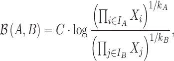The abundance balance between and , denoted by , is defined as the log ratio between the geometric mean abundances of the two groups of taxa:

(3)

where is a normalization constant equal to .

Equivalently, a balance can be rewritten as the difference between the arithmetic means of the log-transformed variables of the two groups of variables:

(4)

where the sign means proportional. A balance is a one-dimensional measure, or score, that summarizes the average log-transformed abundances of two groups of taxa. The larger the value of , the larger the average log abundance of taxa in group compared to the average log abundance of taxa in group . A value of corresponds to the same average log abundance of taxa in groups  and .

Note that balances defined in Equation (3) are referred as isometric log ratios (34) and should not be interpreted as summated log ratios or amalgamation balances that are defined as the log ratio of the total abundance in each group [see (35) for a comparison of these measures].

Selbal

Rivera-Pinto et al. (26) proposed a method for the identification of microbial signatures that are predictive of a phenotype of interest. Unlike approaches that define biomarker signatures as a linear combination of individual markers, the microbial signature from selbal has the form of a balance between two groups of microbial taxa. Selbal seeks for the two groups of taxa and whose relative abundances or balance  is most associated with the outcome of interest according to the following generalized linear model:

(5)

where is the intercept,  is the regression coefficient for the balance score, are additional non-compositional covariates and is the vector of regression coefficients for . The algorithm is implemented for linear and logistic regression.

The optimal balance relies on the identification of taxa that belong to either group A or group B. The first step of selbal algorithm evaluates all possible pairs of taxa to select the pair whose balance is most associated with the response. Then, a forward selection process is performed where, at each step, a new taxon is added to the current balance, either in group A or in group B of the balance to improve the optimization criterion. The objective criterion is defined as the area under the receiver operating characteristic (ROC) curve (AUC) or the proportion of explained deviance for a binary response, and the mean squared error for a linear response. The algorithm stops when there is no remaining variable that improves the optimization criterion or when the maximum number of components in the balance, established with a cross-validation procedure, is reached. Selbal results can be interpreted in terms of microbial balances, an important concept in microbiome studies to describe dysbiosis—a microbial disturbance or imbalance between beneficial and pathogenic microbes, associated with most human disease processes (36,37).

Clr-lasso

Penalized regression is a powerful approach for variable selection in a high-dimensional setting. The estimates of regression parameters are shrunk toward zero by adding a penalized term in the loss function. Variables with a nonzero coefficient are selected as informative variables associated with the outcome variable. Different penalized regression methods exist: the lasso (L₁ norm) puts a constraint on the sum of the absolute values of the regression coefficients, ridge uses the L₂ norm and elastic net uses a linear combination of L₁ and L₂ norms for the penalty term (27,29). A straightforward way of adapting penalized regression methods for CoDA is to first project the compositional data to a Euclidean space, e.g. using the clr transformation:

(6)

where is the geometric mean of the composition.

Interestingly, the clr transformation can be formulated as

(7)

where is the arithmetic mean of the log-transformed values: . Thus, the transformed components are restricted to have a sum equal to zero.

After clr transformation, penalized regression, whether lasso, ridge or elastic net, can be applied. Here, we consider a linear regression model with L₁ penalty, referred as clr-lasso.

For  where is the response and is the composition of k taxa for sample i, clr-lasso is defined as

(8)

The regression coefficients are estimated to minimize

(9)

for a given constant . This is equivalent to minimizing

(10)

where is the penalization parameter. Lasso shrinks some of the regression coefficients to zero, resulting in variable selection of the components with non-null coefficients.

A drawback of this method is that the selection is applied on the clr-transformed variables, which makes interpretation challenging. Equation (8) can be equivalently written as

(11)

(12)

where . Both Equations (11) and (12) show that the term is still present, even after lasso penalization. In other words, although lasso penalization removes irrelevant variables from the regression model, all variables remain in the model through the geometric mean of the clr transformation, . When has a high variance, the power to detect real associations can be reduced and the false discovery rate may increase, as we will explore in our simulation study.

Coda-lasso

An alternative regression approach for CoDA is to consider a log-contrast model (38). This consists in a linear regression model that relates log-transformed covariates with the outcome in the form of a log-contrast function; i.e. the regression coefficients (except the intercept) have a zero-sum constraint, which ensures the scale invariance principle. Such model can be adapted to penalized regression for CoDA variable selection. In the context of microbiome studies, Lin et al. (30) proposed an optimization procedure for penalized linear log-contrast regression models and Lu et al. (31) extended the approach to generalized linear regression models.

Coda linear regression with lasso penalization is formulated as

(13)

with constraint , where the regression coefficients are estimated to minimize

(14)

The minimization process is performed in two iterative steps based on soft thresholding and projection [see (31) for a detailed description].

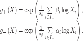
Because of the zero-sum constraint, the fitted regression model can be interpreted as a weighted balance between two groups of components, those with a positive coefficient and those with a negative coefficient, i.e. a log ratio between two weighted geometric means:

(15)

where and are the indices of the positive and negative coefficients, respectively. The parameters are defined as for and . The weighted geometric means are defined as

(16)

Method commonalities

Relationship between clr-lasso and coda-lasso

If we add the constraint to the clr-linear model, the clr transformation cancels out, and clr-lasso is equivalent to coda-lasso:

(17)

since .

Thus, when the regression coefficients are constrained to , the clr transformation is not required and only a log transformation is needed. The regression coefficients inform of the weight of the log-transformed components.

Relationship between selbal and coda-lasso

Similar to coda-lasso, selbal can be expressed as a log-contrast linear model since the sum of the regression coefficients is equal to zero:

(18)

The difference is that the coefficients in selbal for the taxa in each group are all equal to for taxa in group A and for taxa in group B, where and  are the number of taxa in groups A and B, respectively.

Toy example

The similarities and differences between the three methods can be illustrated with a toy example. Let us consider an example where two groups of taxa A and B have been selected for prediction of disease status (cases and controls). Group A is composed of OTU₁ and OTU₂ and group B of OTU₃, OTU₄ and OTU₅. The difference between selbal balance score and coda-lasso balance score is that selbal assigns the same weight to the variables that belong to each group (proportional to the number of variables in each group), while coda-lasso assigns different weights to the taxa. In this example, selbal balance score is given by

and coda-lasso balance score is

where  and  are positive coefficients and and  are negative coefficients, and . For clr-lasso, the linear regression score is of the form

with no restriction on the regression coefficients. This is why, the solution of clr-lasso cannot be considered as a balance as the sum of the regression coefficients is not equal to zero.

Graphical representation

The graphical representation provided by selbal helps interpreting the results, as shown in Figure 1 for the above toy example. The balance score distribution for the controls (in blue) is centered around zero, which means that the average log abundance of group A and group B is similar. On the contrary, the balance score distribution for the cases (in red) is shifted toward positive values; i.e. cases are characterized by a balance with a larger average log abundance in group A than in group B.

Figure 1.

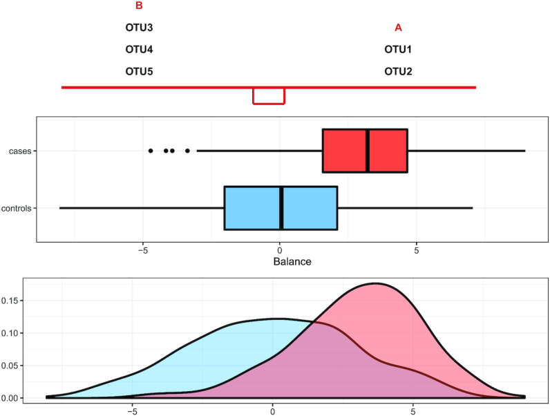
The taxa in group A and group B that constitute the balance. Box plots represent the distribution of balance scores for cases (red) and controls (blue). The density plot of balance scores for cases and controls is shown below.

Similar representation can be extended for coda-lasso, with taxa with a positive regression coefficient assigned to group A and those with a negative regression coefficient assigned to group B.

Implementation

Selbal algorithm is implemented as an R package available on GitHub (https://github.com/UVic-omics/selbal). Clr-lasso first requires a clr transformation [e.g. clr() function in the R package compositions (39)]. Next, penalized regression can be implemented with the R package glmnet (40). An implementation in Matlab of coda-lasso is available in (31). We have developed a new implementation of coda-lasso in R where, similarly to glmnet, the parameter α specifies the ratio between L₁ and L₂ penalization in the elastic net regularization. It is available at https://github.com/UVic-omics/CoDA-Penalized-Regression. A seamless application of all methods on the case studies is available as a reproducible R bookdown vignette on our GitHub page: https://github.com/UVic-omics/Microbiome-Variable-Selection/.

Datasets

High-fat high-sugar diet in mice

The study was conducted by Dr Lê Cao at the University of Queensland Diamantina Institute to investigate the effect of diet in mice. C57/B6 female black mice were housed in cages (three animals per cage) and fed with a high-fat high-sugar diet (HFHS) or a normal diet. Stool sampling was performed at Days 0, 1, 4 and 7. Illumina MiSeq sequencing was used to obtain the 16S rRNA sequencing data. The sequencing data were then processed with QIIME 1.9.0. For our analysis, we considered Day 1 only (HFHS-day1). The OTU (operational taxonomy unit) table after OTU filtering included 558 taxa and 47 samples (24 HFHS diet and 23 normal diet). Both OTU and the taxonomy tables are available on our GitHub page.

Crohn’s disease

The pediatric Crohn’s disease (CD) study (41) includes 975 individuals from 662 patients with CD and 313 without any symptoms. The processed data, from 16S rRNA gene sequencing after QIIME 1.7.0, were downloaded from Qiita (42) study ID 1939. The abundance table was agglomerated to the genus level, resulting in a matrix with 48 genera and 975 samples, which is accessible at our GitHub page.

Simulation study

We evaluated the performance of the three microbiome selection methods according to different scenarios. To mimic as realistically as possible real microbiome data structures, the simulations were based on the two case studies described earlier. The HFHS-day1 dataset exemplifies a scenario, with a large number of taxa (558) and a small number of samples (47), while the CD dataset represents the opposite scenario, with a large number of samples (975) and a moderate number of taxa (48 genera). The simulation process, described in Figures 2 and 3, starts from the original microbiome table, , a matrix of counts or proportions with n rows (samples) and C columns (taxa).

Figure 2.

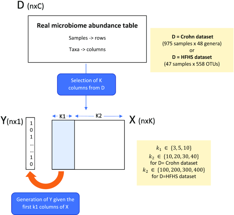
Simulation scheme: the simulated abundance table X is obtained by randomly selecting k columns from the original dataset D. The first k₁ columns of X are used to generate the binary response Y, while the remainder k₂ taxa are deemed irrelevant to explain the outcome. The sizes of K₁ and K₂ vary depending on D.

Figure 3.

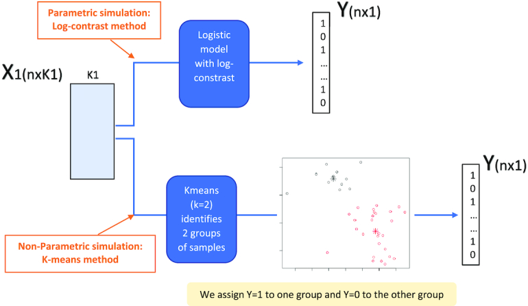
Two schemes were used to generate Y given the K₁ taxa, using a parametric method based on log contrasts, or a non-parametric approach based on K-means.

For each simulation scenario, the abundance table was obtained by randomly selecting k columns (taxa) from the original dataset . The first columns of were used to generate the binary response Y (as described later) and are thus associated with the outcome, while the remainder taxa are not associated with the outcome (since they are not used to simulate Y). The number of taxa associated with the outcome was . This subset of variables is denoted by . The number of taxa non-associated with the outcome, denoted by , was  for the simulations based on the CD dataset and for the simulations based on the HFHS-day1 dataset.

We considered two different schemes for generating the dependent variable : a parametric approach based on a log-contrast model and a non-parametric approach based on K-means method (Figure 3). In the parametric approach, we considered a logistic model with a log-contrast linear regression term by taking the log-transformed variables as covariates and regression coefficients restricted to have a sum equal to zero. This constraint accommodates for the compositional structure of the simulated data. This simulation scheme may favor methods with a similar log-contrast structure such as coda-lasso or selbal. Therefore, we considered a non-parametric simulation scheme based on K-means that consists in calculating the Aitchison distance of the samples using only the  variables, and performing a K-means clustering method with two clusters. This process identifies two groups of samples according to the  taxa abundance profile, where samples within the same group have similar profiles while samples in distinct groups are more different. Samples belonging to cluster 1 were assigned and those belonging to cluster 2 were assigned . Thus, this process constructs a dependent variable that is associated with the  taxa without using a specific parametric model. A detailed description of the simulation scheme is provided in the Supplementary Data. In total, we generated 48 simulated scenarios (2 datasets × 2 methods for generating  × 3 subsets of taxa associated with the outcomes × 4 subsets of non-relevant taxa) that were repeated a hundred times each.

For the three methods, the number of selected variables was determined according to the maximization of the proportion of explained deviance. Methods were then assessed based on the true positive rate (TPR = proportion of associated taxa among the selected variables) and the false positive rate (FPR = proportion of non-associated taxa among the selected variables). These proportions depend on the total number of variables selected by each method, i.e. the penalization parameter  for clr-lasso and coda-lasso. When , no penalization is applied and all variables are selected; thus, TPR = FPR = 1. When is large, no variables are selected and TPR = FPR = 0. We assessed clr-lasso and coda-lasso for a sequence of values of and then obtained TPR( and FPR(. The points (1 − FPR() represent the ROC curve and the AUC provides a summary measure of the accuracy of each method. For selbal, we measured the proportion of true positives and true negatives as a function of the number of selected variables at every step of the forward selection process, and then calculated the AUC of the ROC curve defined by (1 − FPR(TPR() for .

RESULTS

High-fat high-sugar diet in mice

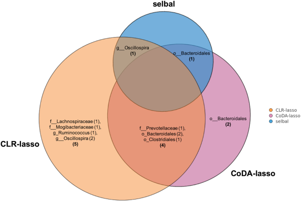
As already described in other studies, e.g. (43), a change from normal to HFHS diet in mice causes rapid alterations in microbiome composition. This was also the case in the HFHS-day1 study, where we observed a strong association between microbiome composition and diet. Selbal identified two taxa whose log ratio perfectly discriminated the two groups of mice (AUC = 1, Figure 4). While selbal was able to achieve maximum discrimination with only 2 taxa, coda-lasso required at least 7 taxa and clr-lasso at least 17 to obtain 100% of explained deviance. For comparison purposes, we set the penalty term for clr-lasso to select 10 taxa (corresponding to 95% of explained deviance). Four variables were selected by both coda-lasso and clr-lasso, while the two variables selected by selbal were in common either with clr-lasso or with coda-lasso (Figure 5).

Figure 4.

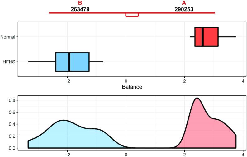
Representation of the distribution of balance values (log ratio) between the two taxa selected by selbal (OTUs 290253 g_Oscillospira and 263479 o_Bacteroidales; f_s24–7) for the mice on an HFHS diet (blue) or normal diet (red) in the HFHS-day1 whole dataset.

Figure 5.

Concordance of the taxa selected by the three methods selbal (blue), clr-lasso (orange) and coda-lasso (pink) for the HFHS-day1 dataset (o = order, f = family and g = genera are indicated depending on available taxonomy).

Most of the bacteria selected by clr-lasso were within the order Clostridiales (7 out of 10) from the families Lachnospiraceae, Mogibacteriaceae and Ruminococcaceae. These families have been found to be associated with high-fat and/or high-sugar diet in mice (44–47). Corroborating these studies, we also found that the relative abundance of Lachnospiraceae was increased in the mice fed with HFHS diet compared to normal diet. Lachnospiraceae consists of pro-inflammatory bacteria (47), which are also reported to be associated with chronic inflammation of the gut (48,49).

The taxa selected by coda-lasso belonged to the order Bacteroidales (6 out of 7) including the family S24-7 (5 out of 6) and Prevotellaceae. The abundance of S24-7 was found to be increased in the diabetes-sensitive mice fed with a high-fat diet, especially after the treatment of remitting colitis in mice (50), while in normal mice, a high-fat diet reduced the abundance of S24-7, which was negatively associated with the inflammatory mediator IL-6 (51). Family Prevotellaceae is able to ferment carbohydrate and protein and was found abundant in obese human individuals (52). In our analysis, the relative abundance of these two families was found to be increased in HFHS diet compared to normal diet.

Selbal selected the genus Oscillospira from order Clostridiales overlapping with clr-lasso, and an unclassified genus from order Bacteroidales overlapping with coda-lasso.

Though selbal selects only two taxa, we emphasize that other taxa are also highly associated with diet in this study. Indeed, in an  setting, it is highly probable that a given balance is not unique and alternative microbial signatures may provide similar results. We investigated other balances by removing the two selected taxa from the dataset and performing selbal again. The method identified a second pair of taxa also with maximum accuracy (AUC = 1 and 100% of explained deviance). The two new selected taxa were both among the variables selected by clr-lasso and one of them among the selected variables by coda-lasso. This case study illustrates the main difference between the methods: selbal seeks for the most parsimonious model with maximum prediction or classification accuracy, while the complexity (i.e. number of variables selected) of clr-lasso and coda-lasso is determined by the penalization parameter. Though penalized regression models are useful for the identification of the variables that are most associated with the outcome, they do not guarantee the best classification performance.

Crohn’s disease

In previous analysis of this dataset with selbal, a balance with 12 variables was determined optimal to discriminate the CD status (26). For ease of comparison, we specified penalized parameters that resulted in the selection of 12 variables for both coda-lasso and clr-lasso. The optimization criterion for fitting the models was the maximization of the proportion of deviance explained.

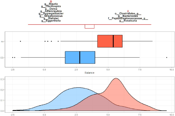
The microbial signature that best discriminates between CD and controls according to selbal is given by the balance between taxa in group A = {o_Clostridiales_g_, g_Bacteroides, f_Peptostreptococcaceae_g_, g_Roseburia} and taxa in group B = {g_Blautia, g_Oscillospira, g_Dorea, g_ Adlercreutzia, g_Streptococcus, g_Dialister, g_Eggerthella, g_Aggregatibacter, g_Adlercreutzia}. The average abundance (geometric mean) of taxa in group A relative to group B is larger in controls than in CD patients (Figure 6).

Figure 6.

Representation of the distribution of balance values (log ratio) between the geometric means of the two taxa groups selected by selbal for CD (blue) and controls (red) in the CD whole dataset.

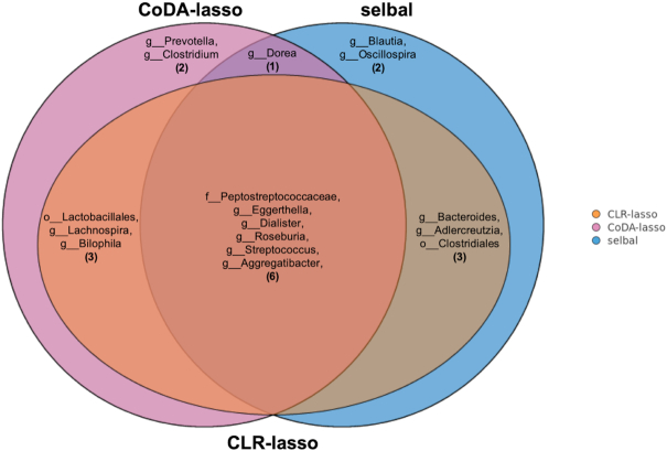
Figure 7 describes the taxa that were selected by the three methods: six taxa in common, seven taxa identified by two methods, two taxa selected solely by selbal and two taxa only by coda-lasso. All the taxa selected by any of the methods have been previously described as markers of inflammation and dysbiosis in CD (41,53–55).

Figure 7.

Concordance of the selected taxa for the CD dataset by the three methods considered: selbal (blue), clr-lasso (orange) and coda-lasso (pink) (f = family; g = genera).

Although the number of variables selected by the three methods was the same, the proportion of explained deviance was considerably larger for selbal (27%) than for clr-lasso (18%) and coda-lasso (21%).

To further assess the classification performance of each method and which taxa signature might be best, we implemented 5-fold cross-validation repeated 20 times, where the signature identified in each training fold was then tested to predict disease status on the test dataset. For each model, or microbial signature, we calculated the ROC curve and the AUC to measure its classification or discrimination accuracy (Figure 8). Selbal microbial signatures led to slightly better classification accuracy than clr-lasso and coda-lasso, which resulted in similar performance.

Figure 8.

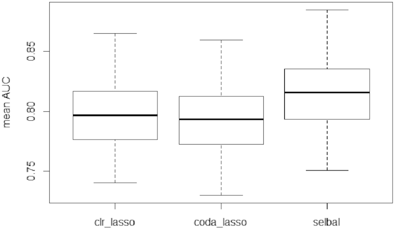
Box plot of the mean AUC of the cross-validation process to evaluate the classification accuracy of clr-lasso, coda-lasso and selbal on the CD dataset.

SIMULATION STUDY

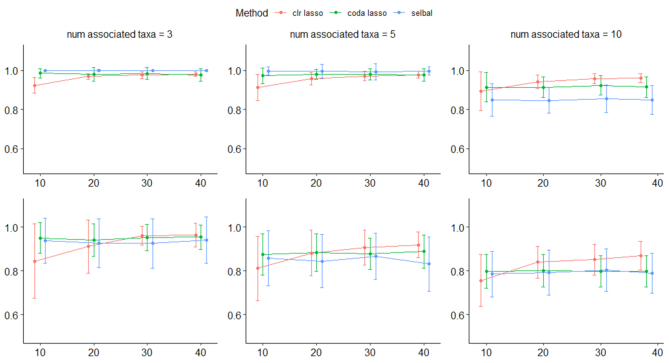
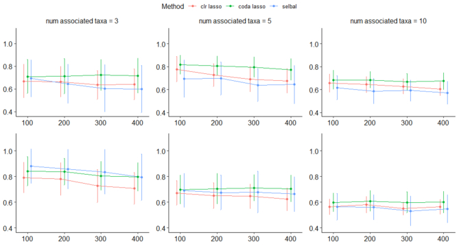
The results of all simulation scenarios are summarized in terms of mean AUC in Figure 9 (simulations based on the CD dataset) and Figure 10 (simulations based on the HFHS-day1 dataset). As expected, we observed a better performance of all methods for the  case (CD dataset) than for the  case (HFHS-day1). In particular, we observed a decrease in performance accuracy when the number of taxa associated with the outcome increased. This can be explained as for a fixed joint effect, the larger the number of discriminant taxa, the smaller their individual contribution.

Figure 9.

Mean AUC for variable selection in the simulations based on the CD dataset for selbal (blue), clr-lasso (red) and coda-lasso (green). The first row corresponds to the log-contrast method to generate Y and the second row to the K-means method. The three columns correspond to the number of taxa associated with Y, , and the x-axis specifies the number of non-associated taxa, .

Figure 10.

Mean AUC for variable selection in the simulations based on the HFHS dataset for selbal (blue), clr-lasso (red) and coda-lasso (green). The first row corresponds to the log-contrast method to generate Y and the second row to the K-means method. The three columns correspond to the number of taxa associated with Y, , and the x-axis specifies the number of non-associated taxa, .

The performance of the methods is highly dependent on the total number of variables in the dataset. In the  scenario (Figure 10), we observed a small decrease in performance of all methods as the total number of variables increases from to , with . In the  scenario (Figure 9), both selbal and coda-lasso had a stable performance as the number of variables increased from to . However, we observed a distinct behavior of clr-lasso: its performance was poor for a small number of variables ( and but improved when k increased. This can be explained by the instability introduced by the clr transformation. Since, , for taxa and sample i, the variability of reduces the power to detect a possible association between the response Y and taxa j. However, as the total number of taxa k increases, the variability of , given by

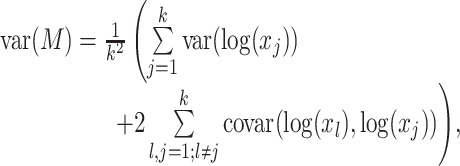(19)

is likely to decrease for large values of because the term in the denominator dominates the numerator in . This is the case, for instance, in the  scenario where the variability of tends to zero when the total number of variables increases (Figure 11). We also observed similar behavior for the HFHS dataset (data not shown).

Figure 11.

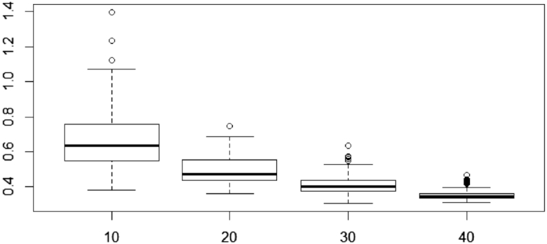
Variability of M after clr transformation [see Equation (19)] for the  scenario, based on the CD dataset. The total number of variables for each simulation scheme is indicated in the x-axis.

DISCUSSION

Variable selection is one of the key procedures in microbiome data analysis. It is relevant for the identification of microbial species that are involved in biological processes or when the interest is the detection of microbial signatures that can serve as biomarkers of disease risk and prognostic (56). The first goal improves biological knowledge and requires precise estimations and control of TPR and FPR. The second goal focuses on classification and prediction: different models can lead to similar prediction accuracy, but parsimonious models can be preferred for their translational use as microbial signatures. It is worth noting that no method can be optimal for both aims.

In this work, we compared three approaches for variable selection in microbiome studies that follow the principles of CoDA, either by considering balances of groups of taxa associated with the outcome (selbal) or with penalized regression after clr transformation (clr-lasso) or constraints on the regression coefficients (coda-lasso). The interpretation of the results is not straightforward in a compositional framework, and we provided practical advice to apply and make sense of the results obtained. In addition, we discussed the different objectives of the approaches we considered. Selbal’s main goal is the establishment of microbial signatures with predictive ability to be used as diagnostic or prognostic markers and thus prioritizes parsimonious models. Penalized regression models seek for the identification of microbial species that in combination relate to the phenotype of interest to increase biological knowledge of the link between disease and microbiome.

Selbal identifies two groups of bacteria whose relative average abundance is associated with the outcome. Such approach is well suited to how we describe microbiome–disease associations in terms of dysbiosis or imbalance between beneficial and pathogenic microbes. In our case studies, Selbal led to better performance than the penalized approaches. In the HFHS dataset, selbal only needed 2 variables to achieve maximum discrimination, while coda-lasso and clr-lasso required 7 and 17, respectively. In the CD dataset, selbal model explained a larger proportion of explained variance and led to slightly higher classification accuracy compared to the other approaches, based on the same selection size. These results can be explained by either a better selection of the features that constitute the signature or the way the microbial signatures are calculated after variable selection. While clr-lasso and coda-lasso regression coefficients are estimated from the training dataset, selbal only retains the set of selected variables and the sign of the coefficients, and each regression coefficient is given by the inverse of the number of variables with either positive or negative sign. Our simulated results suggest that the estimation of coefficients with penalized regression may lead to some overfitting and thus a worse performance than selbal. While this approach is suited for the identification of a predictive microbial signature, it comes with computational cost because of the forward selection process. We propose to apply a combination of selbal with one of the two penalized regression methods to filter the number of variables and lessen the computational burden. This, however, should be done carefully using cross-validation to avoid variable selection bias.

Penalized regression after clr transformation is a valid CoDA approach, but we have identified important drawbacks. Clr penalized regression is not subcompositionally consistent, meaning that different subcompositions will rise to different transformations of the data. Therefore, results are not readily transferable from one study to another where different filtering processes were performed. In addition, microbial signatures obtained from this approach can be difficult to implement on an independent dataset as it raises the question of how the variable from the new dataset should be clr-transformed, and based on which components. The new dataset may include different components, e.g. new taxa not detected in the previous dataset. Most importantly, irrelevant variables are not entirely removed from the analysis: we have shown that all variables remain in the clr transformation term (the geometric mean of all clr-transformed variables).

Clr transformation is algebraically very similar to edgeR and DeSeq2 normalization techniques (57), which suggests that it can be used as library size normalization. However, normalization alone does not solve the compositional issue; thus, univariate testing of clr-transformed variables may result in high FPR when the composition abundances between samples are markedly different.

Using the terminology by Morton et al. (24), the clr transformation uses all taxa as the ‘reference frame’. Such reference may not be suitable in our context as it combines both taxa that are rather stable and taxa that might be quite variable across experimental conditions. The adverse impact of using all taxa as a reference is more evident when the number of taxa is small, as we showed in our simulation study. When , the clr transformation introduces noise and reduces power to detect real associations. When , the clr transformation reduces to an almost constant shift and the analysis is very similar to an analysis of the log-transformed data without any CoDA consideration.

Penalized regression with coefficients restricted to a sum equal to zero, coda-lasso, is an elegant and appropriate CoDA approach. Computation time is efficient and the results can be interpreted as balances between two groups of taxa with weights. However, the determination of the penalty parameter (i.e. the number of variables to retain in the model) is a limitation in this approach. Coda-lasso is suitable to identify variables that are most associated with the outcome though it does not necessary lead to the best accuracy nor the most parsimonious model.

Though not addressed in this work, it is worth noting that, as any CoDA approach, the methods we have assessed rely on logarithms and require handling of zeros. The proportion and nature of the zeros in the dataset will determine the treatment of zeros and also the performance of variable selection methods.

To conclude, users should choose the method that best fits their needs and analysis objectives. Regardless of the approach chosen, we emphasize that variable selection in microbiome studies should be conducted with a multivariate approach that accounts for compositional characteristics, and that the interpretation of the associations of the microbiome with the response variable should be done in terms of balances between groups of bacteria.

SUPPLEMENTARY DATA

Supplementary Data are available at NAR Online.

FUNDING

Catalan Government [2016-DI-013 to M.L.C.]; Spanish Ministry of Economy and Competitiveness [MTM2015-64465-C2-1-R to M.L.C., TIN2017-88515-C2-1-R to A.S.]; Spanish Ministry of Science, Innovation and Universities [BCAM SEV-2017-0718 to M.L.C. and A.S.]; Basque Government [BERC 2018-2021 to M.L.C. and A.S.]; Chinese Scholarship Council (CSC) [to Y.W.]; National Health and Medical Research Council (NHMRC) [GNT1159458 to K.A.L.C.].

Conflict of interest statement. None declared.

REFERENCES

- 1. Calle M.L. Statistical analysis of metagenomics data. Genomics Inform. 2019; 17:e6. [DOI] [PMC free article] [PubMed] [Google Scholar]
- 2. Gloor G.B., Macklaim J.M., Pawlowsky-Glahn V., Egozcue J.J.. Microbiome datasets are compositional: and this is not optional. Front. Microbiol. 2017; 8:2224. [DOI] [PMC free article] [PubMed] [Google Scholar]
- 3. Thorsen J., Brejnrod A., Mortensen M., Rasmussen M.A., Stokholm J., Al-Soud W.A., Sørensen S., Bisgaard H., Waage J.. Large-scale benchmarking reveals false discoveries and count transformation sensitivity in 16S rRNA gene amplicon data analysis methods used in microbiome studies. Microbiome. 2016; 4:62. [DOI] [PMC free article] [PubMed] [Google Scholar]
- 4. Hibbing M.E., Fuqua C., Parsek M.R., Peterson S.B.. Bacterial competition: surviving and thriving in the microbial jungle. Nat. Rev. Microbiol. 2010; 8:15–25. [DOI] [PMC free article] [PubMed] [Google Scholar]
- 5. Gloor G.B., Wu J.R., Pawlowsky-Glahn V., Egozcue J.J.. It’s all relative: analyzing microbiome data as compositions. Ann. Epidemiol. 2016; 26:322–329. [DOI] [PubMed] [Google Scholar]
- 6. Gloor G.B., Reid G.. Compositional analysis: a valid approach to analyze microbiome high-throughput sequencing data. Can. J. Microbiol. 2016; 62:692–703. [DOI] [PubMed] [Google Scholar]
- 7. Quinn T.P., Erb I., Gloor G., Notredame C., Richardson M.F., Crowley T.M.. A field guide for the compositional analysis of any-omics data. GigaScience. 2019; 8:giz107. [DOI] [PMC free article] [PubMed] [Google Scholar]
- 8. Weiss S., Xu Z.Z., Peddada S., Amir A., Bittinger K., Gonzalez A., Lozupone C., Zaneveld J.R., Vázquez-Baeza Y., Birmingham A. et al.. Normalization and microbial differential abundance strategies depend upon data characteristics. Microbiome. 2017; 5:27. [DOI] [PMC free article] [PubMed] [Google Scholar]
- 9. Segata N., Izard J., Waldron L., Gevers D., Miropolsky L., Garrett W.S., Huttenhower C.. Metagenomic biomarker discovery and explanation. Genome Biol. 2011; 12:R60. [DOI] [PMC free article] [PubMed] [Google Scholar]
- 10. Paulson J.N., Stine O.C., Bravo H.C., Pop M.. Differential abundance analysis for microbial marker-gene surveys. Nat. Methods. 2013; 10:1200–1202. [DOI] [PMC free article] [PubMed] [Google Scholar]
- 11. Robinson M.D., McCarthy D.J., Smyth G.K.. edgeR: a Bioconductor package for differential expression analysis of digital gene expression data. Bioinformatics. 2010; 26:139–140. [DOI] [PMC free article] [PubMed] [Google Scholar]
- 12. Love M.I., Huber W., Anders S.. Moderated estimation of fold change and dispersion for RNA-seq data with DESeq2. Genome Biol. 2014; 15:550. [DOI] [PMC free article] [PubMed] [Google Scholar]
- 13. Robinson M.D., Oshlack A.. A scaling normalization method for differential expression analysis of RNA-seq data. Genome Biol. 2010; 11:R25. [DOI] [PMC free article] [PubMed] [Google Scholar]
- 14. Anderson M.J. A new method for non-parametric multivariate analysis of variance. Austral Ecol. 2001; 26:32–46. [Google Scholar]
- 15. Clarke K.R. Non-parametric multivariate analyses of changes in community structure. Aust. J. Ecol. 1993; 18:117–143. [Google Scholar]
- 16. La Rosa P.S., Brooks J.P., Deych E., Boone E.L., Edwards D.J., Wang Q., Sodergren E., Weinstock G., Shannonet W.D.. Hypothesis testing and power calculations for taxonomic-based human microbiome data. PLoS One. 2012; 7:e52078. [DOI] [PMC free article] [PubMed] [Google Scholar]
- 17. Lê Cao K.A., Costello M., Lakis V.A., Bartolo F., Chua X., Brazeilles R., Rondeau P.. MixMC: a multivariate statistical framework to gain insight into microbial communities. PLoS One. 2016; 11:e0160169. [DOI] [PMC free article] [PubMed] [Google Scholar]
- 18. Mandal S., Van Treuren W., White R.A., Eggesbo M., Knight R., Peddada S.D.. Analysis of composition of microbiomes: a novel method for studying microbial composition. Microb. Ecol. Health Dis. 2015; 26:27663. [DOI] [PMC free article] [PubMed] [Google Scholar]
- 19. Fernandes A.D., Macklaim J.M., Linn T.G., Reid G., Gloor G.B.. ANOVA-like differential expression (ALDEx) analysis for mixed population RNA-Seq. PLoS One. 2013; 8:e67019. [DOI] [PMC free article] [PubMed] [Google Scholar]
- 20. Pawlowsky-Glahn V., Egozcue J.J., Tolosana-Delgado R.. Principal balances. Proceedings of the 4th International Workshop on Compositional Data Analysis(CODAWORK). 2011; [Google Scholar]
- 21. Morton J.T., Sanders J., Quinn R.A., McDonald D., Gonzalez A., Vázquez-Baeza Y., Navas-Molina J.A., Song S.J., Metcalf J.L., Hyde E.R. et al.. Balance trees reveal microbial niche differentiation. mSystems. 2017; 2:e00162-16. [DOI] [PMC free article] [PubMed] [Google Scholar]
- 22. Silverman J.D., Washburne A.D., Mukherjee S., David L.A.. A phylogenetic transform enhances analysis of compositional microbiota data. eLife. 2017; 6:e21887. [DOI] [PMC free article] [PubMed] [Google Scholar]
- 23. Washburne A.D., Silverman J.D., Leff J.W., Bennett D.J., Darcy J.L., Mukherjee S., Fierer N., David L.A.. Phylogenetic factorization of compositional data yields lineage-level associations in microbiome datasets. PeerJ. 2017; 5:e2969. [DOI] [PMC free article] [PubMed] [Google Scholar]
- 24. Morton J.T., Marotz C., Washburne A., Silverman J., Zaramela L.S., Edlund A., Zengler K., Knight R.. Establishing microbial composition measurement standards with reference frames. Nat. Commun. 2019; 10:2719. [DOI] [PMC free article] [PubMed] [Google Scholar]
- 25. Quinn T.P., Erb I.. Using balances to engineer features for the classification of health biomarkers: a new approach to balance selection. 2019; 1 May 2019, preprint: not peer reviewed 10.1101/600122. [DOI] [PMC free article] [PubMed]
- 26. Rivera-Pinto J., Egozcue J.J., Pawlowsky-Glahn V., Paredes R., Noguera-Julian M., Calle M.L.. Balances: a new perspective for microbiome analysis. mSystems. 2018; 3:e00053-18. [DOI] [PMC free article] [PubMed] [Google Scholar]
- 27. Tibshirani R. Regression shrinkage and selection via the lasso. J. R. Stat. Soc. Ser. B: Stat. Methodol. 1996; 58:267–288. [Google Scholar]
- 28. Cessie S.L., Houwelingen J.C.V.. Ridge estimator in logistic regression. J. R. Stat. Soc. Ser. C: Appl. Stat. 1992; 41:191–201. [Google Scholar]
- 29. Zou H., Hastie T.. Regularization and variable selection via the elastic net. J. R. Stat. Soc. Ser. B: Stat. Methodol. 2005; 67:301–320. [Google Scholar]
- 30. Lin W., Shi P., Feng R., Li H.. Variable selection in regression with compositional covariates. Biometrika. 2014; 101:785–797. [Google Scholar]
- 31. Lu J., Shi P., Li H.. Generalized linear models with linear constraints for microbiome compositional data. Biometrics. 2018; 75:235–244. [DOI] [PubMed] [Google Scholar]
- 32. Aitchison J. The Statistical Analysis of Compositional Data. 1986; London: Chapman & Hall. [Google Scholar]
- 33. Pawlowsky-Glahn V., Egozcue J.J., Tolosana-Delgado R.. Modelling and Analysis of Compositional Data. 2015; NY: Wiley. [Google Scholar]
- 34. Egozcue J.J., Pawlowsky-Glahn V., Mateu-Figueras G., Barceló-Vidal C.. Isometric logratio transformations for compositional data analysis. Math. Geol. 2003; 35:279–300. [Google Scholar]
- 35. Greenacre M., Grunsky E.C., Bacon-Shone J.. A comparison of amalgamation and isometric logratios in compositional data analysis. 2019; 11 May 2020, preprint: not peer reviewedhttps://www.researchgate.net/publication/332656109.
- 36. Carding S., Verbeke K., Vipond D.T., Corfe B.M., Owen L.J.. Dysbiosis of the gut microbiota in disease. Microb. Ecol. Health Dis. 2015; 26:26191. [DOI] [PMC free article] [PubMed] [Google Scholar]
- 37. Sheflin A.M., Whitney A.K., Weir T.L.. Cancer-promoting effects of microbial dysbiosis. Curr. Oncol. Rep. 2014; 16:406. [DOI] [PMC free article] [PubMed] [Google Scholar]
- 38. Aitchison J., Bacon-Shone J.. Log contrast models for experiments with mixtures. Biometrika. 1984; 71:323–330. [Google Scholar]
- 39. van den Boogaart K.G., Tolosana-Delgado R.. “Compositions”: a unified R package to analyze compositional data. Comput. Geosci. 2008; 34:320–338. [Google Scholar]
- 40. Friedman J., Hastie T., Tibshirani R.. Regularization paths for generalized linear models via coordinate descent. J. Stat. Softw. 2010; 33:1–22. [PMC free article] [PubMed] [Google Scholar]
- 41. Gevers D., Kugathasan S., Denson L.A., Vázquez-Baeza Y., Van Treuren W., Ren B., Schwager E., Knights D., Song S.J., Yassour M. et al.. The treatment-naïve microbiome in new-onset Crohn’s disease. Cell Host Microbe. 2014; 15:382–392. [DOI] [PMC free article] [PubMed] [Google Scholar]
- 42. Gonzalez A., Navas-Molina J.A., Kosciolek T., McDonald D., Vázquez-Baeza Y., Ackermann G., DeReus J., Janssen S., Swafford A.D., Orchanian S.B. et al.. Qiita: rapid, web-enabled microbiome meta-analysis. Nat. Methods. 2018; 15:796–798. [DOI] [PMC free article] [PubMed] [Google Scholar]
- 43. Hildebrandt M., Hoffmann C., Sherrill-Mix S.A., Keilbaughlow S.A., Hamady M., Chenlow Y., Knight R., Ahima R.S., Bushman F., Wu G.D.. High-fat diet determines the composition of the murine gut microbiome independently of obesity. Gastroenterology. 2009; 137:1716–1724. [DOI] [PMC free article] [PubMed] [Google Scholar]
- 44. Zhao R., Khafipour E., Sepehri S., Huang F., Beta T., Shen G.X.. Impact of Saskatoon berry powder on insulin resistance and relationship with intestinal microbiota in high fat–high sucrose diet-induced obese mice. J. Nutr. Biochem. 2019; 69:130–138. [DOI] [PubMed] [Google Scholar]
- 45. Muhomah T.A., Nishino N., Katsumata E., Haoming W., Tsuruta T.. High-fat diet reduces the level of secretory immunoglobulin A coating of commensal gut microbiota. Biosci. Microbiota Food Health. 2019; 38:55–64. [DOI] [PMC free article] [PubMed] [Google Scholar]
- 46. Sanguinetti E., Collado M.C., Marrachelli V.G., Monleon D., Selma-Royo M., Pardo-Tendero M.M, Burchielli S., Iozzo P.. Microbiome-metabolome signatures in mice genetically prone to develop dementia, fed a normal or fatty diet. Sci. Rep. 2018; 8:4907. [DOI] [PMC free article] [PubMed] [Google Scholar]
- 47. Voigt R.M., Forsyth C.B., Green S.J., Mutlu E., Engen P., Vitaterna M.H., Turek F.W.. Circadian disorganization alters intestinal microbiota. PLoS One. 2014; 9:e97500. [DOI] [PMC free article] [PubMed] [Google Scholar]
- 48. Zeng H., Ishaq S.L., Zhao F.Q., Wright A.D.G.. Colonic inflammation accompanies an increase of β-catenin signaling and Lachnospiraceae/Streptococcaceae bacteria in the hind gut of high-fat diet-fed mice. J. Nutr. Biochem. 2016; 35:30–36. [DOI] [PubMed] [Google Scholar]
- 49. Kläring K., Just S., Lagkouvardos I., Hanske L., Haller D., Blaut M., Wenning M., Clavel T.. Murimonas intestini gen. nov., sp. nov., an acetate-producing bacterium of the family Lachnospiraceae isolated from the mouse gut. Int. J. Syst. Evol. Microbiol. 2015; 65:870–878. [DOI] [PubMed] [Google Scholar]
- 50. Ormerod K.L., Wood D.L.A., Lachner N., Gellatly S.L., Daly J.N., Parsons J.D., Dal’Molin C.G.O., Palfreyman R.W., Nielsen L.K., Cooper M.A. et al.. Genomic characterization of the uncultured Bacteroidales family S24-7 inhabiting the guts of homeothermic animals. Microbiome. 2016; 4:36. [DOI] [PMC free article] [PubMed] [Google Scholar]
- 51. Pyndt Jørgensen B., Hansen J.T., Krych L., Larsen C., Klein A.B., Nielsen D.S., Josefsen K., Hansen A.K., Sørensen D.B.. A possible link between food and mood: dietary impact on gut microbiota and behavior in BALB/c mice. PLoS One. 2014; 9:e103398. [DOI] [PMC free article] [PubMed] [Google Scholar]
- 52. Zhang H., DiBaise J.K., Zuccolo A., Kudrna D., Braidotti M., Yu Y., Parameswaran P., Crowell M.D., Wing R., Rittmann B.E. et al.. Human gut microbiota in obesity and after gastric bypass. Proc. Natl Acad. Sc. U.S.A. 2009; 106:2365–2370. [DOI] [PMC free article] [PubMed] [Google Scholar]
- 53. Shaw K.A., Bertha M., Hofmekler T., Chopra P., Vatanen T., Srivatsa A., Prince J., Kumar A., Sauer C., Zwick M.E. et al.. Dysbiosis, inflammation, and response to treatment: a longitudinal study of pediatric subjects with newly diagnosed inflammatory bowel disease. Genome Med. 2016; 8:75. [DOI] [PMC free article] [PubMed] [Google Scholar]
- 54. Pascal V., Pozuelo M., Borruel N., Casellas F., Campos D., Santiago A., Martinez X., Varela E., Sarrabayrouse G., Machiels K. et al.. A microbial signature for Crohn’s disease. Gut. 2017; 66:813–822. [DOI] [PMC free article] [PubMed] [Google Scholar]
- 55. Wright E.K., Kamm M.A., Teo S.M., Inouye M., Wagner J., Kirkwood C.D.. Recent advances in characterizing the gastrointestinal microbiome in Crohn’s disease: a systematic review. Inflamm. Bowel Dis. 2015; 21:1219–1228. [DOI] [PMC free article] [PubMed] [Google Scholar]
- 56. Knights D., Parfrey L.W., Zaneveld J., Lozupone C., Knight R.. Human-associated microbial signatures: examining their predictive value. Cell Host Microbe. 2011; 10:292–296. [DOI] [PMC free article] [PubMed] [Google Scholar]
- 57. Quinn T.P., Erb I., Gloor G., Richardson M.F., Crowley T.M.. Understanding sequencing data as compositions: an outlook and review. Bioinformatics. 2018; 34:2870–2878. [DOI] [PMC free article] [PubMed] [Google Scholar]
Associated Data
This section collects any data citations, data availability statements, or supplementary materials included in this article.