

Abstract
Despite its importance as a clinical imaging modality, magnetic resonance imaging remains inaccessible to most of the world’s population due to its high cost and infrastructure requirements. Substantial effort is underway to develop portable, low-cost systems able to address MRI access inequality and to enable new uses of MRI such as bedside imaging. A key barrier to development of portable MRI systems is increased magnetic field inhomogeneity when using small polarizing magnets, which degrades image quality through distortions and signal dropout. Many approaches address field inhomogeneity by using a low polarizing field, approximately ten to hundreds of milli-Tesla. At low-field, even a large relative field inhomogeneity of several thousand parts-per-million (ppm) results in resonance frequency dispersion of only 1 – 2 kilohertz. Under these conditions, with necessarily wide pulse bandwidths, fast spin-echo sequences may be used at low field with negligible subject heating, and a broad range of other available imaging sequences can be implemented. However, high-field MRI, 1.5T or greater, can provide substantially improved signal-to-noise ratio and image contrast, so that higher spatial resolution, clinical quality images may be acquired in significantly less time than is necessary at low-field. The challenge posed by small, high-field systems is that the relative field inhomogeneity, still thousands of ppm, becomes tens of kilohertz over the imaging volume. This article describes the physical consequences of field inhomogeneity on established gradient- and spin-echo MRI sequences, and suggests ways to reduce signal dropout and image distortion from field inhomogeneity. Finally, the practicality of currently available image contrasts is reviewed when imaging with a high magnetic field with large inhomogeneity.
Keywords: Field inhomogeneity, portable MRI, frequency-swept
Graphical Abstract
1. Introduction
Nowadays magnetic resonance imaging (MRI) is an indispensable tool in biomedical research and clinical medicine. Yet, due to its expense and infrastructure requirements, access to MRI is restricted to mainly wealthier nations and institutions, which limits point-of-care applications. For example, Ogbole et al. [1] found that only 84 MRI units served approximately 372,551,411 people across the West African sub-region. Of those, 58 were in Nigeria and 14 in Ghana, with all other countries in the region having 3 or fewer MRI units. The 0.48 MRI units/million people in Ghana gives it the highest concentration of MRI units in the region. Compared to the 22.4 MRI units/million people in the United States [2], the low concentration found in the West African sub-region is dismal. As a result, significant efforts and resources are currently devoted toward devising new approaches to decrease the size and cost of MRI, while maximizing image quality and reducing scan times.
To accomplish these goals, recent efforts have focused on approaches that allow MRI to be performed with relatively nonuniform static fields (B0), as occurs when 1) shrinking the magnet size relative to the imaging volume [3–8], 2) using open or single-sided magnets [9–11], or 3) ramping the polarizing B0 up and then down for signal readout in ultralow field [12–14]. Decreasing the physical magnet size or using an open design both have the benefit of requiring less superconductor and magnet mass. As a result, these systems are usually easier to transport and less costly to site and operate than standard clinical magnets. At the same time, the ever-increasing demand for high signal-to-noise ratio (SNR) and spatial resolution continually drives the development of higher field systems, further exacerbating the field inhomogeneity problem. In general, as a magnet’s size decreases, bore space for high-power active shim sets also decreases, which limits the ability to correct the magnetic field. Fortunately, MR imaging with large B0 inhomogeneity is a manageable problem, since the field inhomogeneity, ΔB0, is generally smoothly varying within the imaging volume, with the exception of large ΔB0 generated by metallic implants. The effects of smoothly varying ΔB0 can be either compensated or overcome using various techniques described herein, while imaging near metallic implants, which can be particularly challenging due to large ΔB0 variation over small spatial scales, will be elaborated on later in this article.
For imaging with open magnet designs, sequences such as Stray Field Imaging (STRAFI) [9] or NMRMouse [10, 11, 15] may be more applicable than those described herein. However, those methods generally require physical translation of the object inside the magnet to generate a full image and are generally not practical for imaging humans. Approaches to decrease magnet size typically revolve around low-field systems, where the polarizing field is generated from permanent magnet arrays. Permanent magnet systems need no cryogens and in some cases can be extremely lightweight relative to superconducting systems, with one example being the MR cap that weighs just 8.3 kg [5]. Among the most popular designs for permanent magnet arrays is the Halbach array [16], which Blümler and others began popularizing as early as 2004 [17–19]. Cooley et al. [4] demonstrated MRI at 77.3 mT with a Halbach array and by using static field gradients for encoding. The performance of that system was later improved using a genetic algorithm to optimize the magnet design [3]. A new approach to Halbach array design with the genetic algorithm was recently published by O’Reilly et al. [8] with a mean field of 50.4 mT. A new permanent magnet design, specifically using an Aubert ring pair [20] , recently achieved a polarizing field of 169.7 mT [7], significantly stronger than the aforementioned Halbach systems. A substantial advantage of low-field (low-frequency) systems is that the specific absorption rate (SAR) limits are, in practice, rarely reached [21].
Unfortunately, the spatial and temporal resolution of permanent magnet systems are limited by the low polarizing field. For example, the MR Cap achieved ~2-mm in-plane resolution with a 6-mm slice thickness in 11 minutes with the RARE sequence [22]. A detailed analysis of possible sequence adjustments to tradeoff tissue contrast, SNR, and spatial resolution in low-field MRI is described by Marques et al. [21]. Similar low resolution images (2.5 × 3.5 × 8.5 mm3) were obtained by Sarracanie et al. [23] with a balanced steady-state free precession sequence in a 6.5 mT polarizing field generated by an electromagnet. As argued therein [23], low-field MRI is a promising, low-cost avenue to provide clinically relevant images which complement high-field MRI without supplanting it.
We therefore are focused on reducing the cost of and barriers to high-field (≥1.5T) MRI by enabling clinical quality imaging using magnets having large and spatially smooth B0-variation. Such field variation approximately describes the useable volume of small, high-field, high-temperature superconducting (HTS) magnets [24]. Similar to permanent magnet arrays, HTS magnets obviate the need for cryogens and can instead be chilled by low power cryo-coolers [25]. However, performing high-quality MRI in the presence of large field inhomogeneity presents major challenges. Fortunately, many of those can be overcome, as we describe herein.
2. Mathematic Preliminaries
In the mathematical descriptions presented herein, all vectors are denoted by boldface letters, such as x. For ease of reading, when denoting the spatial gradient of the field inhomogeneity, we use as opposed to ∇ΔB0(x).
3. Issues Posed by Field Inhomogeneity
Below, spin excitation and refocusing are treated separately from spatial encoding methods to more thoroughly treat the distinct intricacies of the issues posed by large field inhomogeneity.
3.1. Excitation and Refocusing
3.1.1. Pulse Options:
Clinical MRI typically requires the peak-to-peak magnetic field homogeneity to be constrained to within 2 – 3 parts per million (ppm), such that the resonance frequency dispersion at 1.5T or 3T is on the order of 200 – 400 Hz. Such uniform fields permit the use of narrow-band radiofrequency (RF) pulses which can reasonably excite or refocus the entire imaging volume, or well-delineated slices, typically with a bandwidth less than 1 kHz. In contrast, at ultra-high field, here defined as ≥7T, the inhomogeneity is typically greater than 1400 Hz wth 5 ppm peak-to-peak field inhomogenetiy. With novel small or open magnet designs [24], the field inhomogeneity can easily reach 200 – 300 ppm, equivalent to as much as 10 – 20 kHz at 1.5T.
To facilitate spin manipulation at these latter bandwidths, conventional amplitude-modulated (AM) pulses are no longer sufficient. For a given flip angle, AM pulses have a fixed time-bandwidth product, TBP( = Δω · TP, where TP is the duration and Δω is the bandwidth of the pulse). As such, the bandwidth can only be increased by shortening the pulse, requiring a higher amplitude to achieve the same flip angle. At the bandwidths mentioned above, the required RF amplitude needed for large flip angle pulses exceeds the capabilities of standard RF amplifiers. From a practical standpoint then, frequency-modulated (FM) pulses are required to overcome this issue, whereby the instantaneous frequency of the pulse is swept in time through the full bandwidth of the pulse [26, 27]. Frequency sweeping distributes the RF energy in time, so that high-bandwidth excitation and refocusing can be achieved with low peak RF amplitude. Additionally, for a fixed amplitude-modulation function, the bandwidth of the pulse can be altered by changing the frequency (or phase) modulation function of the pulse. Hence, a pulse need not be made shorter to increase the bandwidth.
At the large bandwidths used herein, spin-echo sequences may become impractical due to limits on SAR and subject heating. Even with frequency-swept pulses, obtaining the RF amplitude necessary for a 180° refocusing pulse can be, in practice, unachievable, or at best, difficult. Using flip angles <180° is a viable option, at the expense of mixed T1 and T2 image contrast. While established spin-echo methods are covered later in this article, more advanced imaging sequences are also discussed to achieve RF refocusing with low flip angles outside of conventional spin-echo sequences.
3.1.2. Spatial Selection:
In conventional MRI, signal can be made to originate from only a localized region in space (i.e., a slice or slab) by using spatially selective excitation pulses. This is done by applying an RF pulse in the presence of a linear field gradient, after which the gradient area, or moment, must be nulled (refocused) by applying a gradient with opposite polarity. The need for refocusing manifests more clearly in the small-tip-angle approximation [28], where the magnetization profile, e.g. the complex transverse magnetization, is expressed as the Fourier transform of a weighted sampling function in a spatial frequency space, k-space. Mathematically, the Fourier relationship is expressed as
| (1) |
Here, W(k) is a weighting function reflecting k-space sampling density and S(k) is the k-space sampling function. The gyromagnetic ratio is denoted by γ. Of particular note in Eq. (1) is the relationship between the k-space coordinate k(t) and the gradient G(t) applied during the pulse, that is
| (2) |
In Eq. (2), T is the duration of the gradient waveform used for excitation, while t’ is a dummy integration variable over time. Note the integration is evaluated from the current time t through the end of the excitation. The k-space coordinate is given by the integral of the remaining gradient, not by the integral of the gradient which has already occurred.
The implications of the above are extremely important: whenever the RF pulse samples k = 0, the integral of the remaining gradient at that time must be 0 to properly refocus the transverse magnetization. For a symmetric RF pulse which samples k = 0 halfway through the pulse duration, the remaining gradient integral during the pulse is half the overall integral. Hence, only half the gradient integral needs to be refocused. For asymmetric pulses, different amounts of refocusing are necessary.
In light of the above, in the presence of unknown field inhomogeneity, slice refocusing becomes exceedingly difficult. Consider the application of an RF pulse of duration TP in the presence of a static unknown linear field inhomogeneity GU in the same direction as the applied slice select gradient G, immediately followed by a refocusing interval ending at time T, as shown in Fig. 1.
Figure 1:
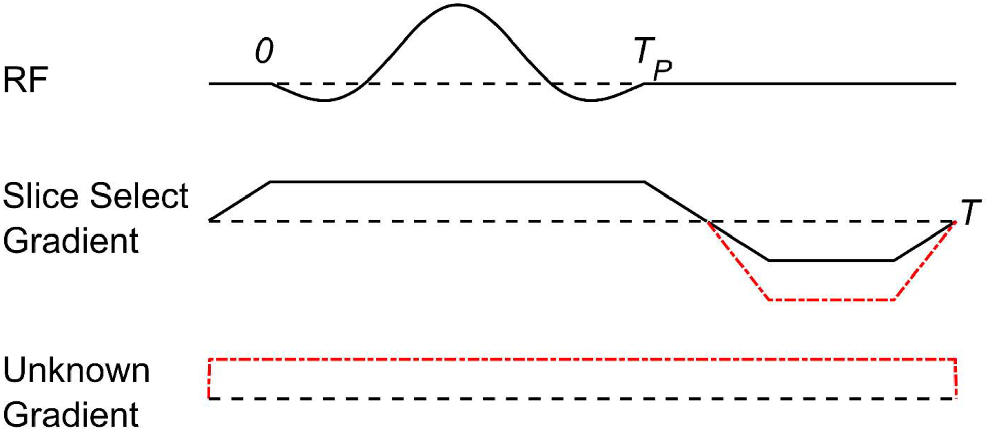
A 1D concept diagram of slice selection in the presence of an unknown field inhomogeneity, GU. The solid (black) gradient line denotes the slice select gradient amplitude necessary for proper refocusing without field inhomogeneity. The dot-dashed (red) line denotes the slice select amplitude necessary for refocusing in the presence of the static unknown gradient.
The k-space coordinate during a symmetric excitation pulse in this situation is
| (3) |
Following the pulse, only the applied gradient polarity can be reversed for refocusing, while the unknown gradient would continue traversing k-space in the same direction. The center of the RF pulse is then not applied at k = 0, but at the displaced position
| (4) |
Such improper slice refocusing leads to net signal loss, since the transverse magnetization within the slice is not all in phase at the end of the excitation. When ignoring system-dependent gain terms and potential slice profile distortions, the net signal magnitude |sdisplaced| following the pulse is
| (5) |
Considering Eq. (5), an approximate quantitative estimate of the amount of signal loss can be made by assuming a perfect box-car excitation profile. Without loss of generality, the slice is assumed to be at x = 0 and has thickness L. Assuming the magnitude of the transverse magnetization does not vary significantly through the plane of the slice, the signal magnitude is
| (6) |
Hence, a sinc function approximates the signal loss as a function of slice thickness and the degree to which the slice is not refocused. In practice, it is quite common for kdisplaced to inhibit any measurable signal from a voxel. Therefore, the use of slice or slab selection is not recommended when significant field inhomogeneity exists, as full refocusing cannot be guaranteed without using another RF (refocusing) pulse and unavoidable signal loss occurs. While another RF pulse could be used to refocus the slice, as discussed earlier, performing refocusing pulses with large field inhomogeneity may exceed safe levels of RF deposition (SAR).
3.1.3. Slice Profile Distortion:
In the absence of any field inhomogeneity, the resonance frequency of a spin at position x in the presence of a gradient G is given by ω = γ G · x. With field inhomogeneity, the resonance frequency is shifted to
| (7) |
where Ĝ denotes a unit vector in the direction of G. From Eq. (7), the position of excited spins shifts along the applied gradient by , graphically illustrated in Fig. 2. Hence, stronger gradients for slice selection result in less slice displacement.
Figure 2:
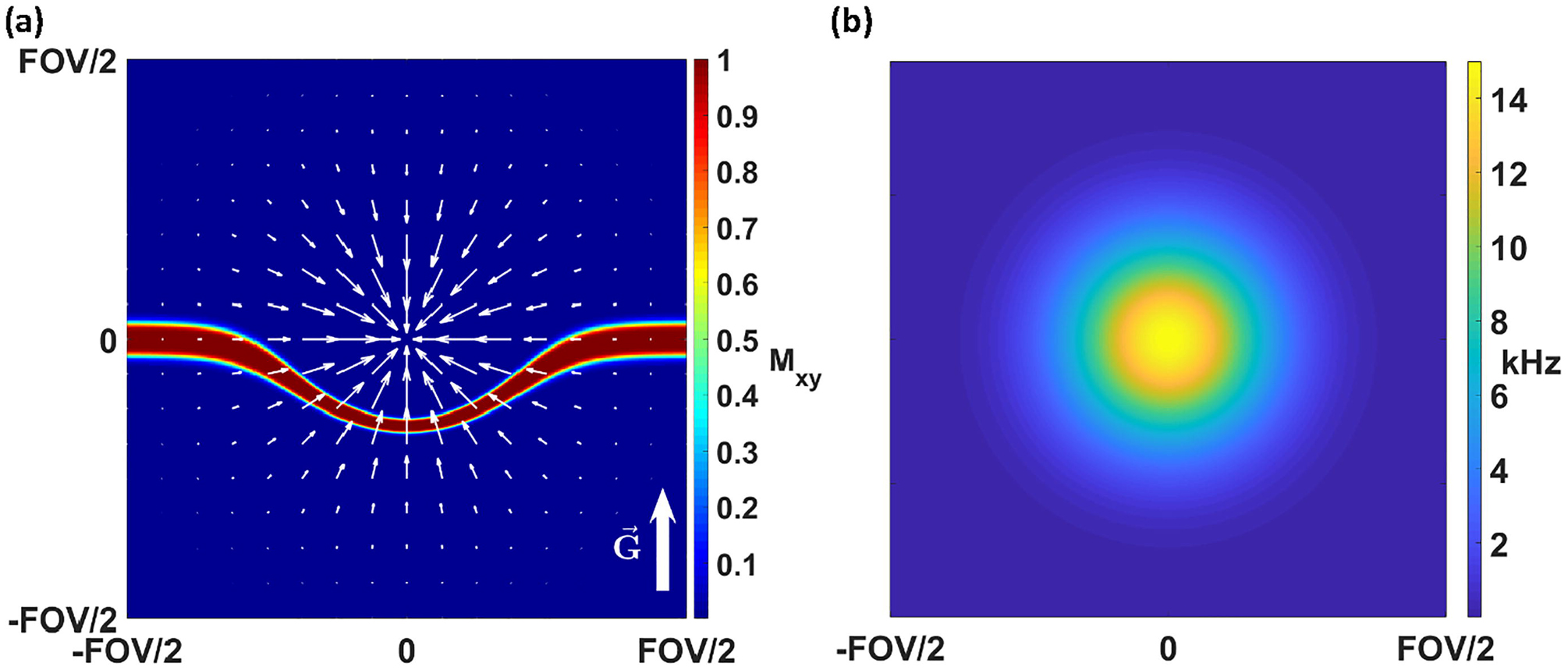
Simulation of slice distortion in an inhomogeneous B0 field. (a) Slice profile when applying a slice selective gradient in the presence of an inhomogeneous field. The superimposed white arrows indicate the magnitude and direction of the inhomogeneity gradient, while the labeled white arrow in the lower right indicates the applied slice select gradient direction. (b) The bell-shaped B0 field used for this simulation.
However, not only does the slice shift, the slice thickness also becomes a function of position. With zero field inhomogeneity, and pulse bandwidth Δω, the nominal slice thickness is given by . With field inhomogeneity, slice thickness becomes
| (8) |
In positions where the applied gradient G and the inhomogeneity gradient are collinear, the denominator in Eq. (8) increases, causing the slice to thin - see Fig. 2. If the directions of the applied gradient and inhomogeneity gradient are opposed, the slice widens. Clearly, Eq. (8) reverts back to the standard expression for slice thickness when . Further insight is gained by factoring the applied gradient out of Eq. (8) to give
| (9) |
In the form of Eq. (9), it is evident that increased gradient strength also decreases the influence of field inhomogeneity on slice thickness modulation. For a fixed nominal slice thickness , the bandwidth of the RF pulse must increase commensurately with the gradient to maintain slice thickness. Thus, a general approach to mitigate slice profile distortion is to use the highest bandwidth RF pulses permissible and corresponding gradient strengths for a desired slice thickness, within SAR and hardware constraints.
3.2. Spatial Encoding
We begin this section by discussing the induced image distortion caused by field inhomogeneity. Later, signal dropout resulting from echo shifts induced by field inhomogeneity is examined.
3.2.1. Background:
The ability to resolve the spatial structure of objects in MRI is achieved by spatial encoding with linear field gradients. From Faraday’s law of induction [29, 30], the signal in MRI is given by
| (10) |
when ignoring relaxation effects. Here, the signal, s, is parameterized as a function of discrete sampling time, tn, while the integration volume is over the sensitive region of the receive coil(s). Inverting the Fourier relationship in Eq. (10) yields discrete approximations to the continuous object Mxy(x). Thus, when confounding factors such as relaxation, off-resonance, motion, etc. are absent, image reconstruction is as simple and efficient as applying an inverse Fast Fourier Transform (FFT) to the signal.
The spatial frequency function k(t), which parameterizes acquisition k-space, is notably different here than in the case of excitation described above. Now,
| (11) |
No longer is the integral evaluated over the remaining gradient waveform. Rather, it is evaluated over the gradient waveform which has already occurred. This assumes an appropriate origin in time has been chosen - that is, after the refocusing of excitation gradients. Due to its relatively long readout period consisting of multiple gradient echoes, echo-planar imaging (EPI) [31] is extremely sensitive to field inhomogeneity. Two problems occur with long acquisition time. First, magnetic field inhomogeneity (ΔB0) and susceptibility variation in the object leads to diminished signal amplitude (also called dephasing) during the long acquisition readout, and this acts as a k-space filter, reducing the effective resolution of the image [32, 33]. The second problem relates to EPI’s low acquisition bandwidth in the phase-encoded (blipped) dimension, producing large image distortion with only small ΔB0 [34, 35].
3.2.2. Single Point Phase Encoding:
With the exception of rapid imaging techniques such as EPI, phase encoding is typically performed by collecting one k-space point along the phase encoded direction per RF pulse. As this does not preclude encoding other axes, this section will only consider a 1D phase-encoded example.
The relationship between the k-space increment Δk and the field-of-view (FOV) of the reconstructed image is perhaps one of the most important relationships:
| (12) |
If all phase-encoding gradients are applied for the same amount of time, τ, with linearly distributed amplitudes, an alternative expression for Δk is
| (13) |
In the absence of field inhomogeneity, with N acquired phase-encoding steps, the nth signal is
| (14) |
with and . It has been assumed without loss of generality that N is even. As discussed earlier, the image is then the inverse FFT of the sequence sn.
For a gradient echo sequence with echo time TE in the presence of spatially-varying field inhomogeneity ΔB0(x), the signal becomes
| (15) |
Modest rearrangement of Eq. (15) gives,
| (16) |
Since the inner term of the integrand in Eq. (16) does not depend on the index n, the inverse Fourier transformation of sn yields the image Mxy(x)exp (−i γ ΔB0(x) TE), which is simply the original image Mxy(x) multiplied by a unit magnitude phase factor. No image distortion occurs due to the field inhomogeneity in phase-encoded directions [36]. However, with gradient echo sequences, signal dropout still occurs due to intravoxel dephasing, an approximation of which is given in Eq. (6).
3.2.3. Frequency Encoding:
Analyzing again the case of a gradient echo sequence, loosely following the analysis of Chang & Fitzpatrick [37], the 1D frequency-encoded signal is given by
| (17) |
Here, and tn is constructed such that the center of the data acquisition period is at TE. Denoting the acquisition time as Ta, the discrete sampling times are , again with . Rearranging Eq. (17) gives
| (18) |
Defining a distorted coordinate
| (19) |
and the Jacobian
| (20) |
Eq. (18) becomes
| (21) |
Thus, the image is distorted by the field inhomogeneity ΔB0(x), since the distorted image Mxy(x′)exp (−i γΔB0(x′) TE)J−1(x′) forms a Fourier pair with the signal. Another important factor, the inverse of the Jacobian J has also appeared. The Jacobian describes the degree of image intensity pileup or dropout due to voxels stretching and compressing, respectively, under the action of the field inhomogeneity.
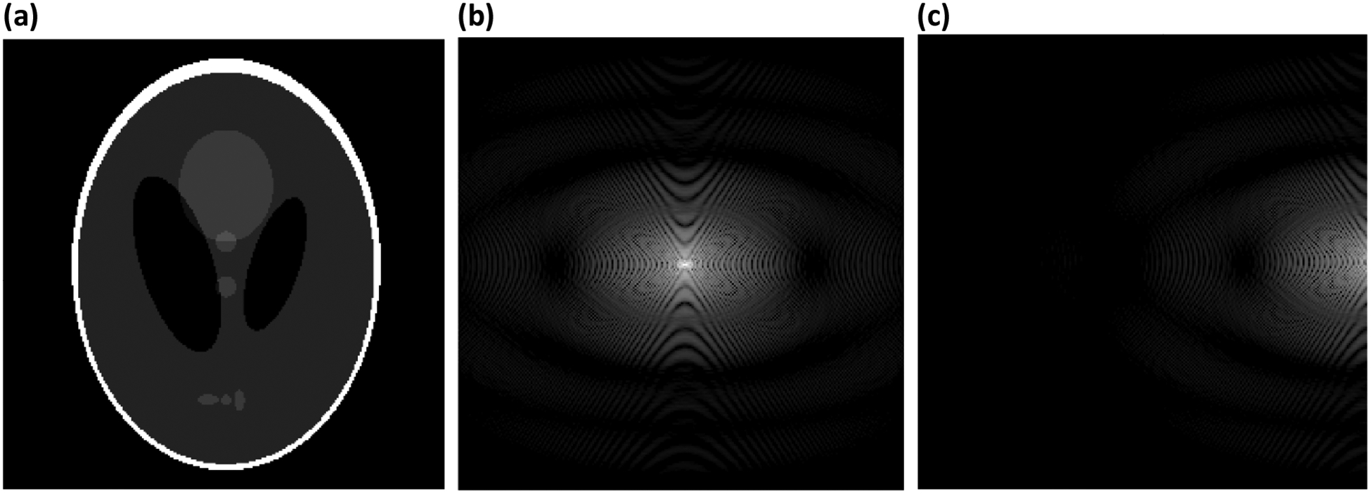
Importantly, the inverse Jacobian appears in Eq. (21), so the Jacobian must always be positive, never zero. The physical significance of the Jacobian being zero amounts to the local field gradient being of equal in magnitude but opposite in sign to the applied field gradient. When this occurs, there is no spatial encoding at that point in space. The lack of spatial encoding causes voxels in the reconstructed image to “stretch”, containing more signal than a voxel otherwise would without field inhomogeneity, causing hyperintense volumes in the reconstructed image. The opposite case occurs when the local and applied field gradients have the same sign, causing rapid frequency variation over a small spatial scale. In this case, voxels shrink in the readout direction, causing signal dropout (areas of hypo-intensity) in the reconstructed image. As appropriately characterized by Reichenbach et al. [36], the field inhomogeneity changes the local FOV due to the combined action of the applied and local field gradient in the frequency-encoded direction. A simulation of these effects is shown in Fig. 3.
Figure 3:
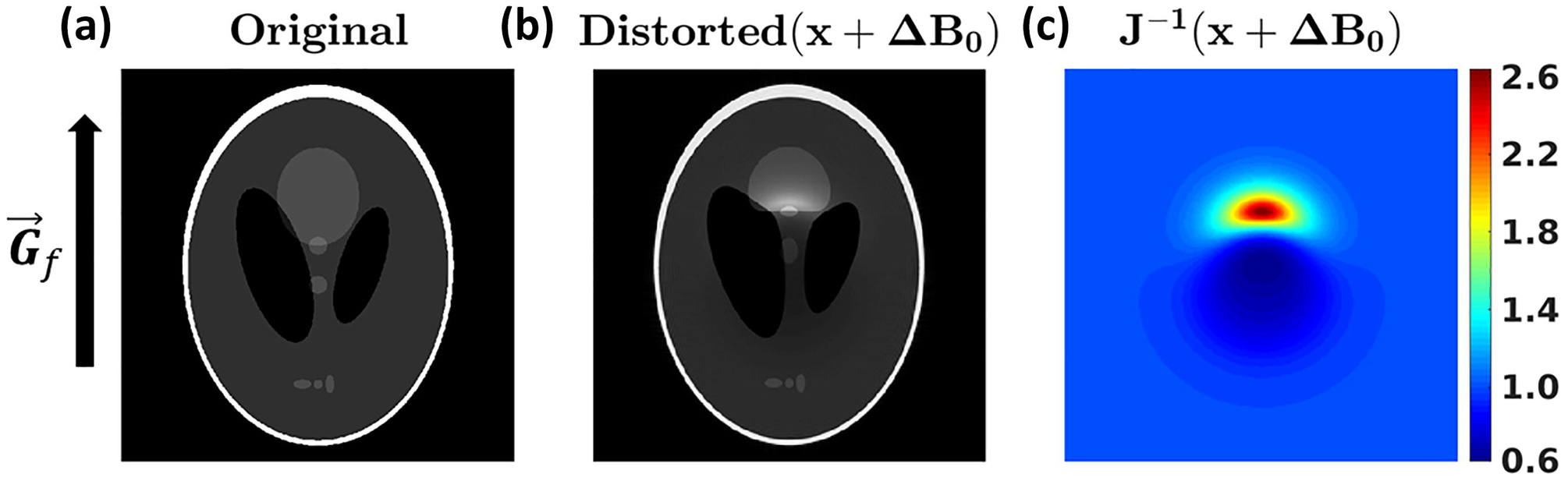
Demonstration of the effects of ΔB0 on a simulated reconstruction. The frequency-encoding direction is vertical, as indicated. (a) The original Shepp-Logan phantom [38] used for simulation. (b) The results of a Bloch simulation, showing the large distortions due to ΔB0. (c) The inverse Jacobian of the transformation sampled on the distorted coordinates, as indicated by Eq. (19). The Jacobian aligns well with the hyper- and hypo-intense regions of (b).
From Eqs. (19) and (20), an increased readout gradient strength dampens the geometric and intensity distortions stemming from the field inhomogeneity. Further insight in this regard is made by connecting the frequency-encoding gradient strength to more conventional user-controlled parameters, e.g. the FOV and receiver bandwidth sw. Using Eqs. (12) and (13) gives . Then for a fixed , so a larger frequency-encoding gradient necessitates a larger receiver bandwidth. With a fixed FOV and number of samples, the increased sw shortens the acquisition time, decreasing the signal-to-noise ratio (SNR) according to [39].
3.2.4. Correcting Distortions in Frequency-encoded Direction
If ΔB0(x) is measured, for example using a double-echo [40] or chemical shift imaging sequence [41], the image distortion and intensity correction can be mostly corrected [42]. Possible correction steps, given graphically in Fig. 4, are as follows: 1) Calculate the Jacobian of the distortion induced by ΔB0(x); 2) Interpolate the geometric and intensity distorted image onto a uniform grid to correct geometric distortions; 3) Intensity correct the image by multiplication with the Jacobian. To avoid unphysical discontinuities in the directly measured ΔB0(x) map, it is generally wise to smooth the map, either by polynomial fitting or fitting to smooth basis functions [43]. Alternatively, given ΔB0(x), an inverse problem can be posed to solve for the corrected image [44].
Figure 4:
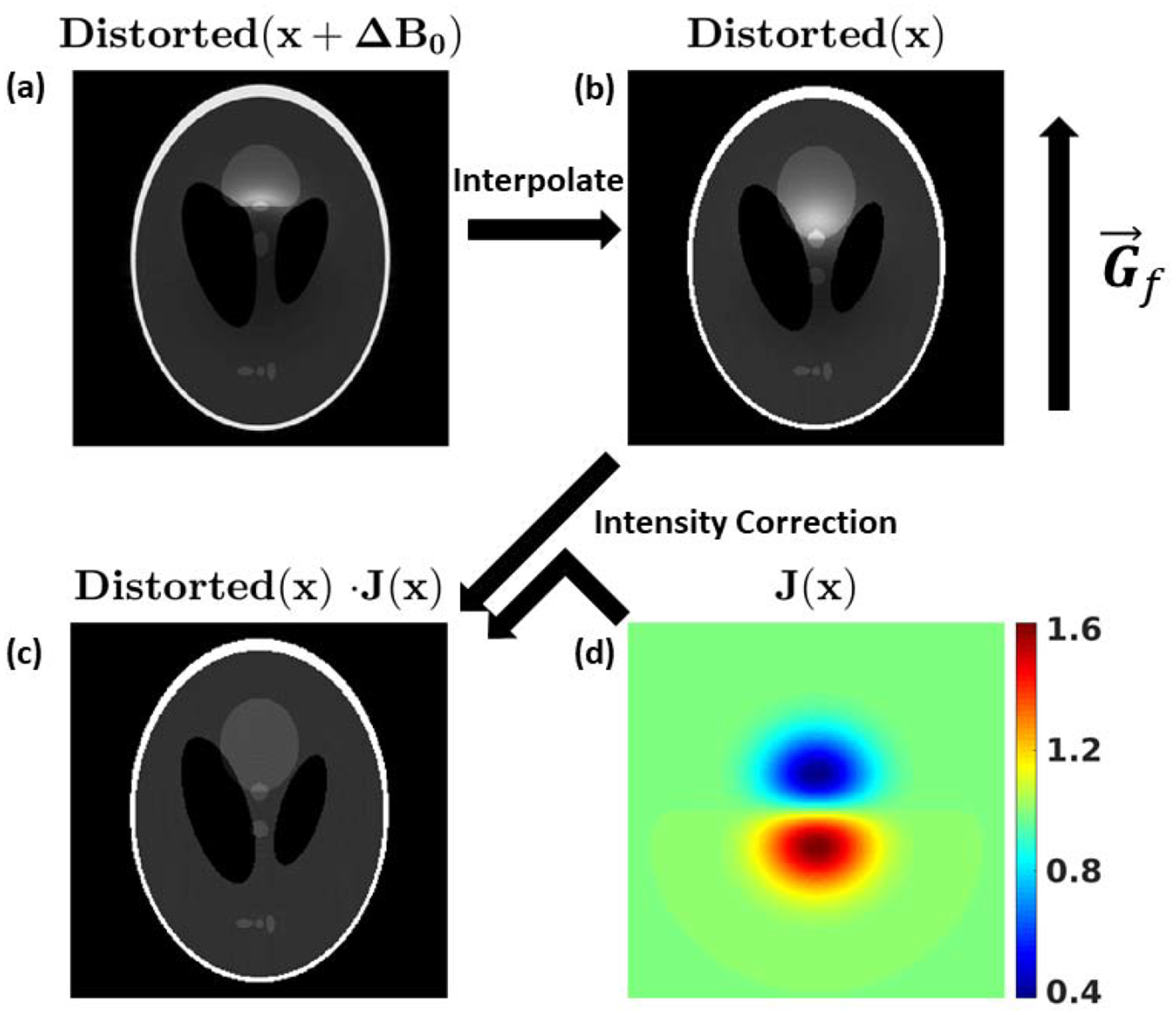
Overview of the steps necessary to correct ΔB0 distortions. The same ΔB0 was used here as in Fig. 2. (a) The intensity and geometrically distorted image sampled on the distorted coordinates. Interpolating (a) according to a measured ΔB0 map yields (b). The intensity distorted image, now sampled on the desired coordinates. Combining (b) with (d), the Jacobian of the distortion map, yields the final image (c), which is mostly free of distortions.
3.2.5. Spatial Selection Revisited: Echo shifting
An effective approach to compensate for field inhomogeneity when using spatially-selective RF pulses is to acquire the same slice with various amounts of slice refocusing, as shown in Fig. 5. The underlying motivation for this lies in Eq. (3), where the amount of dephasing across the slice is unknown. Thus, performing slice refocusing with a large range of gradient moments will, at some point, refocus the slab. This approach is called gradient-echo slice excitation profile imaging (GESEPI) [45], where it is noted that performing slice refocusing in this manner is tantamount to phase encoding. However, in GESEPI, the 3D dataset which has been Fourier transformed in the slice dimension, is necessarily summed over the slice dimension to reduce the image back to 2D. Using GESEPI for 2D imaging therefore requires excess time to encode each slice multiple times in the slice direction. For short repetition time (TR) sequences, where slice interleaving is not possible, this causes a proportional increase in scan duration. Therefore, when performing short TR gradient echo sequences in the presence of large field inhomogeneity, it is advantageous to directly perform 3D imaging with a high resolution in the slice (or slab) dimension, as discussed immediately below.
Figure 5:
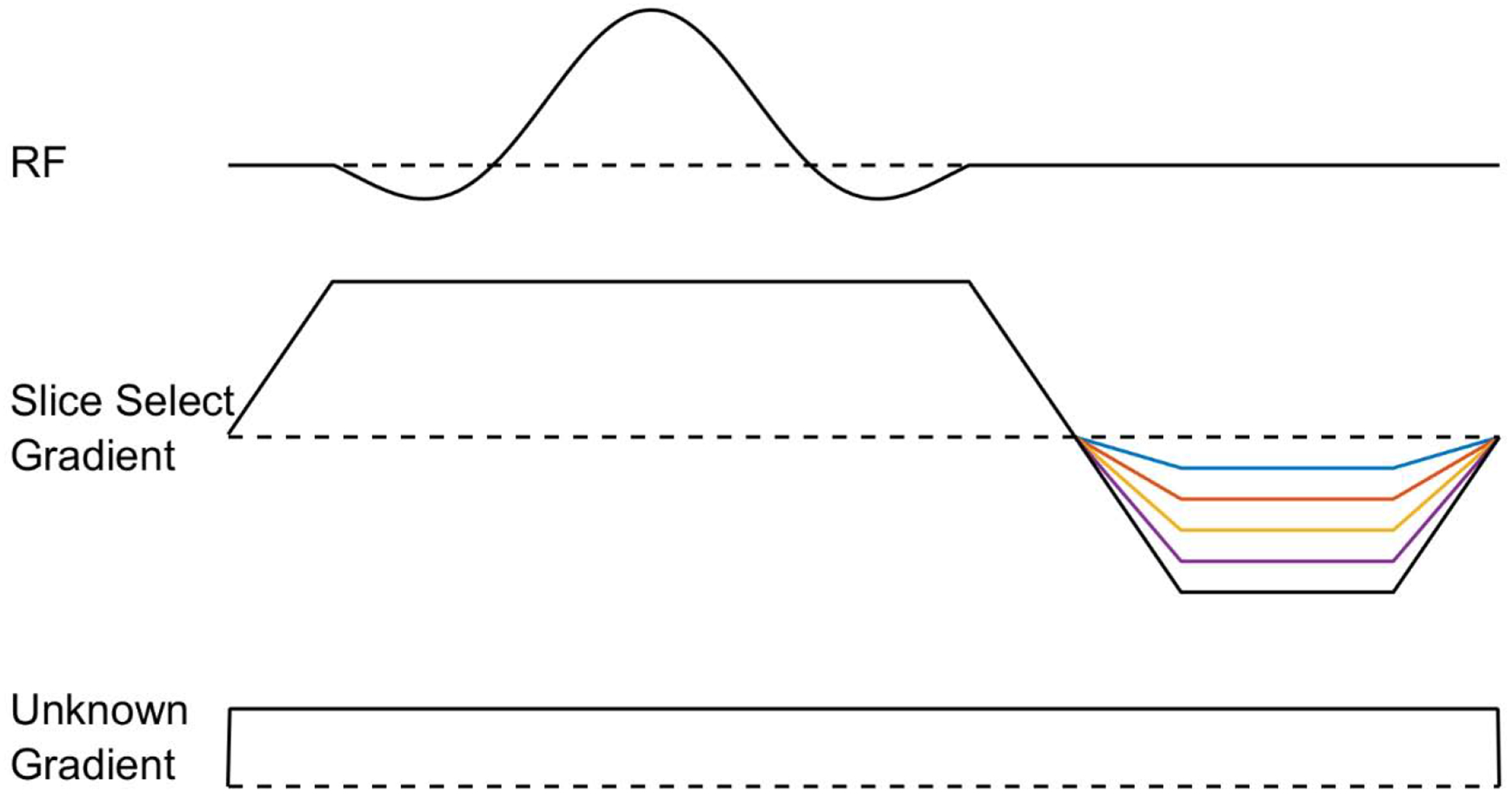
A concept diagram for gradient echo slice excitation profile imaging (GESEPI) in the presence of an unknown field inhomogeneity. An array of 2D images is collected with various amounts of slice refocusing with the aim of refocusing all voxels in the selected dimension over the course of the experiment.
In 3D, consider the signal due to a single uniform voxel with transverse magnetization Mxy, centered at position x0, and of width L on all sides. In the absence of any applied gradients during excitation and treating the field inhomogeneity as linearly varying over the voxel, e.g. , the signal magnitude is given by
| (22) |
Above, the following identifications have been made, with the time origin placed at the center of the RF pulse:
| (23a) |
| (23b) |
One interpretation of the above is that the center of k-space, where peak signal amplitude occurs, has shifted by the amount −kB0(t), as that is where the exponent in the integrand of Eq. (22) evaluates to zero [36]. Per Eq. (22), the echo at position x0, which would be the k-space origin without field inhomogeneity, now occurs at kapplied(t) = −kB0(t) instead of at kapplied(t) = 0. Thus, so long as the echo for a given voxel lies within , the echo will be measured for that voxel. In other words, higher resolution imaging increases the likelihood of measuring the echo for all voxels [46]. If this condition is not satisfied, the center of the echo is not captured, reducing the amount of signal from the voxel under consideration.
A key feature of Eq. (23a) is that shorter echo times result in a higher likelihood of measuring the echo from any given voxel. A short echo time also leaves less time for spins within the voxel to dephase under the action of the field inhomogeneity, kB0(t), before data acquisition. Moreover, a short echo time is more readily achieved with a short RF pulse, which decreases the contribution to the echo shift originating from the RF pulse, as seen in Eq. (23a).
For the three directions n = x,y,z, evaluating the integral in Eq. (22) for a single voxel results in the following expression for signal magnitude:
| (24) |
In Eq. (24), [k]n indicates the nth component of the vector k and . It can then be guaranteed that the echoes from all voxels are sampled if none of the sinc functions of Eq. (24) cross zero for any voxel. That is, for all voxels
| (25) |
or
| (26) |
In Eq. (26), the limiting spatial frequency is , with exactly 2π radians of phase variation across a voxel. Thus, if the combined effect of the field inhomogeneity and the imaging gradients never produce a fully dephased voxel, most of the signal energy originating from that voxel will still be measured during acquisition. This is a further demonstration of how higher resolution images mitigate the signal loss stemming from field inhomogeneity; as L→0, the spatial frequency necessary to reach 2π variation over any voxel tends to ∞.
If the field inhomogeneity term kB0(t) effects an additional π phase variation or more across a particular voxel, the applied field gradients will be unable to measure the echo for that voxel. Fig. 6 demonstrates the case where the field inhomogeneity induces a π phase variation across all voxels in the image. Note that a shift in k-space where the peak amplitude occurs for a voxel forces asymmetric sampling of k-space, where the distal lobes of the sinc functions in Eq. (24) are small. This results in a modest amount of signal loss relative to the case of no field inhomogeneity, which is examined quantitatively later.
Figure 6:
Simulation showing the effects of B0 inhomogeneity on the sampling of k-space. (a) The Shepp-Logan phantom [38] used in the simulation. (b) log image of the k-space magnitude with no field inhomogeneity. (c) log image of k-space with , demonstrating the inability to sample the echo (at what is traditionally kapplied = 0).
4. Sequences: What Works?
4.1. Gradient Echo Imaging
Earlier, it was shown that phase-encoded dimensions are not distorted in MRI, and that signal loss can be mitigated using short echo times and non-selective RF pulses. An apparent first candidate imaging sequence might therefore be a high bandwidth, non-selective excitation followed by 3D phase encoding, as is done in Single-Point Imaging (SPI) [47, 48], Single-Point Ramped Imaging with T1 Enhancement (SPRITE) [49, 50], or in some versions of chemical shift imaging [51]. However, SPI methods are notoriously inefficient in time, as they collect only one data point per RF pulse. For a short repetition time, say 5 ms, at a clinically relevant spatial resolution, 1 mm3, and FOV = 256 × 192 × 192 mm3, the total scan time would be approximately 13 hours without acceleration. Additionally, SPI uses a high gradient duty cycle, resulting in significant noise and vibration, which is uncomfortable for living subjects. Clearly the long scan time with elevated vibration and noise is not practical for routine use.
Alternatively, if a modest amount of image distortion is acceptable, a short echo time gradient echo sequence can be used with frequency encoding in one dimension with a high receiver bandwidth [36, 52]. While the high receiver bandwidth in general decreases the SNR, the increased SNR at high-field and/or with receiver arrays [53] aids in offsetting losses due to the increased receiver bandwidth. A notable remark is that the overall approach remains the same: short echo time and a non-selective excitation. Using the same repetition time, resolution, and FOV as described in the preceding paragraph, such an imaging sequence would take approximately 3 minutes to run, a vast improvement over 13 hours. Earlier, the signal energy shift in k-space under the action of a field inhomogeneity was presented. Now consider the human brain images in Fig. 7, which were acquired in a well-shimmed 1.5T magnet using a 3D GRE sequence without selective excitation. The k-space data are nearly symmetric about the origin of k-space, as indicated by the lines through kapplied = 0, also showing where each k-space cross section is taken. The SNR of this image was 12.68, calculated using two 10 × 10 × 10 voxel regions-of-interest (ROI), one in a region of no signal, and one in a region of relatively uniform signal [54, 55], indicated in Fig. 7.
Figure 7:
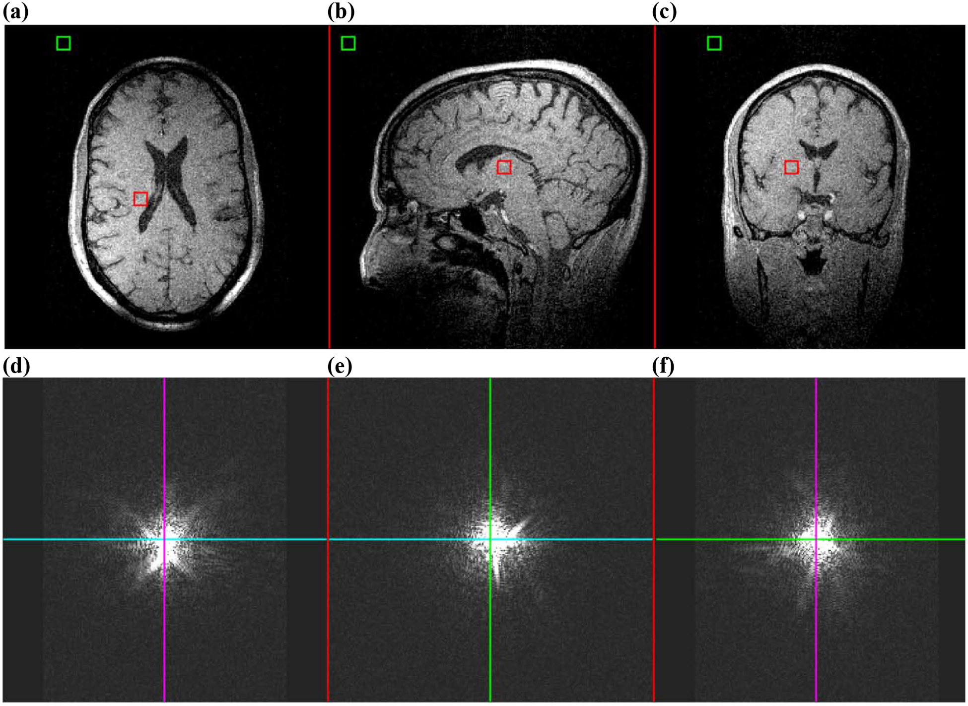
Image and k-space data for a 3D GRE taken with a well-shimmed field at 1.5T and measured with 1 mm isotropic resolution. The repetition and echo times were TR/TE = 10ms/4.3ms, the receiver bandwidth was 151.52 kHz, and FOV = 256 × 192 × 256 mm3. a – c) Cross sections through isocenter. d – f) Cross sections of k-space for the same dataset. The colored lines indicate where each cross section in k-space is taken through the other dimensions. Images were generated by 3D FT prior to k-space data zero-padding, which was done for aesthetic purpose only.
An inhomogeneous field can be obtained by intentionally mis-setting one linear shim for the duration of the experiment. Here, the static offset was approximately 0.1508 G/cm, or greater than 12 kHz variation in resonance frequency over the brain. In this scenario, the result, particularly in k-space, is much more interesting - see Fig. 8.
Figure 8:
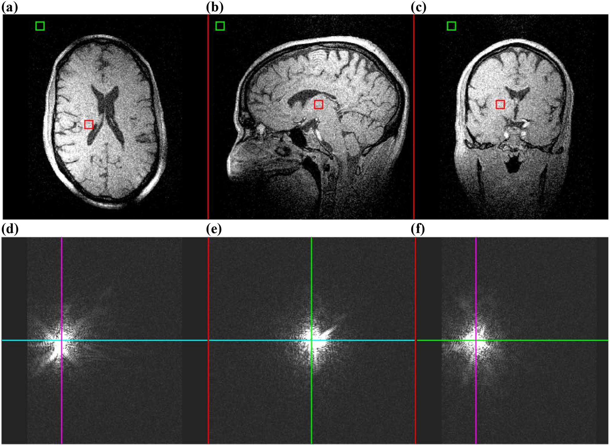
Image and k-space data for a 3D GRE taken with a poorly-shimmed field at 1.5T and measured with 1 mm isotropic resolution. The repetition and echo times were TR/TE = 10ms/4.3ms, the receiver bandwidth was 151.52 kHz, and FOV = 256 × 192 × 256 mm3. a – c) Cross sections through isocenter. d – f) Cross sections of k-space for the same dataset. The colored lines indicate where each cross section in k-space is taken through the other dimensions. Images were generated by 3D FT prior to k-space data zero-padding, which was done for aesthetic purpose only.
Clearly, the peak amplitude in k-space has shifted, as it is no longer symmetric about kapplied = 0, particularly in the direction that was phase encoded (left-right from the subject’s perspective). In image space, besides obvious spatial mis-registration, there is some less apparent blurring due to the field inhomogeneity. In this experiment, the field inhomogeneity was linear and orthogonal to the applied frequency-encoding gradient, thereby tilting the direction of frequency encoding relative to the intended axis by . Here, GΔ denotes the shim gradient acting as a field inhomogeneity, while Gapplied is the applied frequency-encoding gradient. The encoded axes in k-space are then not all mutually orthogonal, resulting in blurring [56]. Using the same calculation method [54, 55], the SNR of this image was 12.54, a loss of only 1.1% relative to the well-shimmed case.
4.2. Spin-Echo Imaging
As discussed above, spin-echo imaging does not suffer from -decay as gradient-echo imaging does. However, there are still issues of slice distortion with selective pulses and image distortion in the frequency-encoding dimension. Subject heating is also a primary concern with spin-echo imaging with large field inhomogeneity due to the necessarily large pulse bandwidths used. This section serves as a brief overview of established methods, their benefits, and limitations.
4.2.1. View angle tilting
One of the simplest techniques for overcoming field inhomogeneity in spin-echo sequences is view angle tilting (VAT) [57]. VAT uses a compensation gradient in the slice direction to correct for slice distortion and frequency-encoding distortions resulting from susceptibility and chemical shift effects. In principle, while the slice is distorted by field inhomogeneity, the compensation gradient maps spins to a set of coordinates distorted in the opposite direction to that of the slice distortion. The ideal case is where the compensation and frequency-encoding gradients have the same magnitude, in which case the compensation gradient maps the slice back to its true position. The sequence diagram is shown in Fig. 9.
Figure 9:
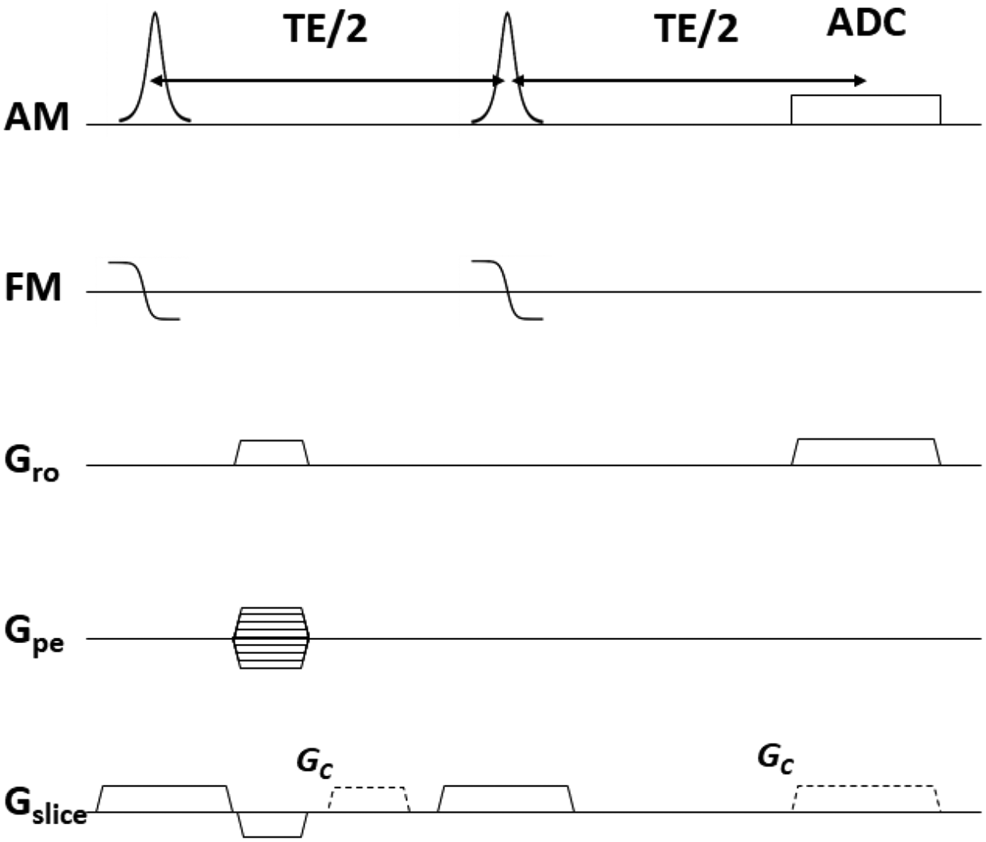
The sequence diagram for view angle tilting. AM and FM denote the amplitude and frequency modulation functions of the RF waveform, respectively, Gro denotes the applied readout gradient, Gpe denotes the applied phase encoding gradient, and Gslice denotes the applied slice-selection gradient. Compensation gradients in the slice direction, Gc, are shown as dashed lines. Ideally, the compensation and frequency-encoding gradients are of equal magnitude.
By orienting the frequency-encoding axis out of the plane of the slice, a significant amount of blurring is introduced. As Butts et al. demonstrated [58], the blurring can be mitigated by matching the sampling time to the duration of the main lobe of the excitation RF pulse. Conventionally in MRI, the sampling time is generally longer than the main lobe of the RF pulse. To match the durations, there are two clear choices: 1) Increase the receiver bandwidth to decrease the sampling time at the expense of SNR, or 2) Increase the pulse duration at the expense of decreased pulse bandwidth. For option (2), low-bandwidth RF pulses increase slice distortions, exacerbating the exact problem which VAT is meant to address. Therefore, as Butts et al. [58] suggested and demonstrated, using FM excitation pulses as a means to increase pulse bandwidth without decreasing the pulse duration is ideal, as the receiver bandwidth can then be left unchanged. Another key assumption of VAT is that the field inhomogeneity does not vary significantly in the through-plane direction, which is not necessarily true for thicker slices, although practically this does not have a substantial impact.
4.2.2. Slant-slice
A technique conceptually similar to VAT is slant-slice imaging. If the field inhomogeneity is linear and limited to being primarily along one direction, it can be used as a component of the gradients used for both slice selection and frequency encoding [56]. Without loss of generality, consider the permanent gradient GP to be along the z direction, while an experimentally controlled gradient GX is applied orthogonal to GP, as in Fig. 10. For slice-selection, GX is applied with positive polarity and is reversed for frequency encoding. The slice is excited at an angle θ to the z-axis and the frequency-encoding gradient is elevated an angle α out of the slice plane. The ideal scenario is that |GX| = |GP| such that the angle and α = 0 in Fig. 10. Specifically, in the ideal case the slice select gradient and frequency-encoding gradient are completely orthogonal.
Figure 10:
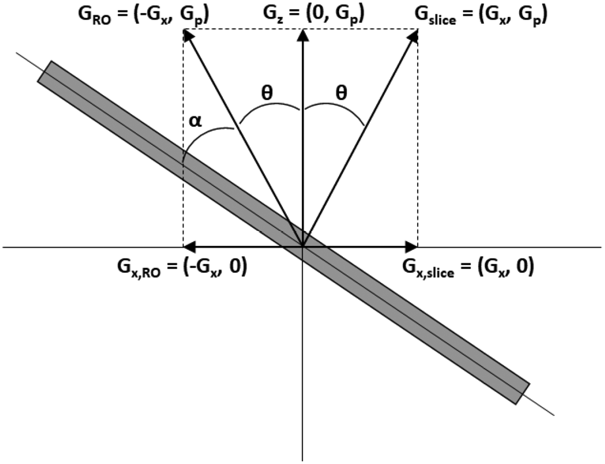
A conceptual diagram showing the principle of slant-slice imaging. A permanent gradient GP along z is used as a component of both the slice select gradient Gslice and as a component of the frequency-encoding gradient GRO. A controlled gradient GX is toggled between positive and negative polarities for slice selection and frequency encoding, respectively.
As a spin echo sequence, the refocusing pulse permits complete slice refocusing despite the presence of field inhomogeneity. Combined with the Modified Driven Equilibrium Fourier Transform (MDEFT) spin-echo sequence [59], slant-slice imaging can yield high-quality T1-weighted images, despite approximately 80 kHz field inhomogeneity over the brain, as shown in Fig. 11.
Figure 11:
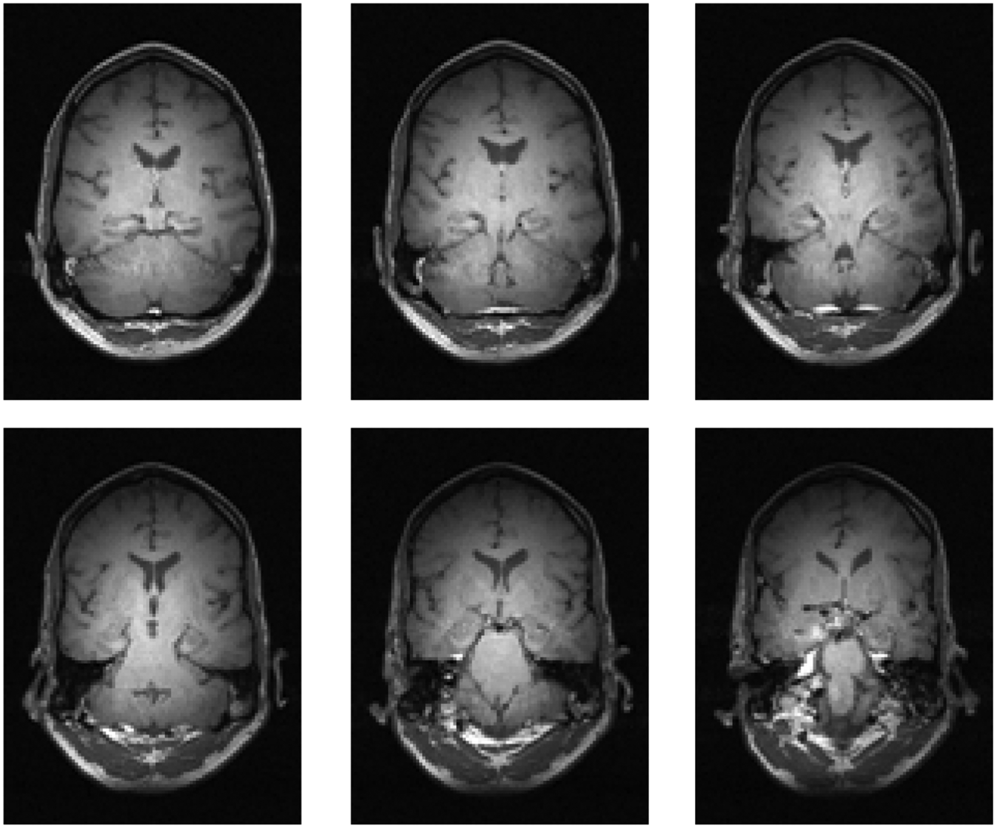
A selection of 6 slices from a 16-slice set taken at 4T with the slant-slice MDEFT sequence. The slice thickness was 2.5 mm and in-plane resolution was 1 mm. A constant gradient was applied for the duration of the experiment, inducing an 80 kHz resonance frequency variation over 25 cm.
The most significant drawback of slant-slice imaging is its sensitivity to nonlinear variations in the static field, a situation common in many MRI applications. To an extent, the large gradients used for slice-selection and frequency encoding alleviate this problem, but yield lower SNR. Another potential issue is the unusual oblique image orientation, which may not be familiar to many radiologists. As a 2D multislice sequence, there is little guarantee of the ability to resample a set of slices onto a 3D volume for reorientation to a clinical standard.
4.2.3. Multispectral Approaches
Herein we have repeatedly discussed the challenges of properly exciting and refocusing large bandwidths in MRI. Near metallic implants, these challenges are only increased, as the assumption of a large but slowly varying field inhomogeneity no longer holds. Metallic implants induce large field inhomogeneities which are localized in space, going from on the order of −10 kHz to 10 kHz in a matter of centimeters. To address this unique challenge, two new approaches were developed to image only narrow bandwidths at a given time. The first technique, multi-acquisition variable-resonance image combination (MAVRIC) [60], is a 3D fast spin-echo (FSE) sequence utilizing narrowband, spectrally selective RF pulses with distributed center frequencies. This permits separate imaging of narrow spectral bins to fully cover the entire off-resonance range [60]. With MAVRIC, the spectral bins are generally excited with spectrally-selective boxcar-type profiles and refocused with Gaussian pulses. Additionally, the bins are made to overlap by approximately one half the bandwidth of the RF pulses. The Gaussian spectral profile permits smooth bin combination, limiting image intensity artifacts in the bin-combined image at the spatial locations where spectral bins overlap, as demonstrated in Fig. 12. The advantage of boxcar excitation profiles is that they allow independent excitation of separate spectral bins. Without spatially-selective pulses, MAVRIC is a relatively slow technique, even with the FSE-type acquisition. To obtain clinically relevant scan times and spatial resolution, large acceleration factors are necessary.
Figure 12:
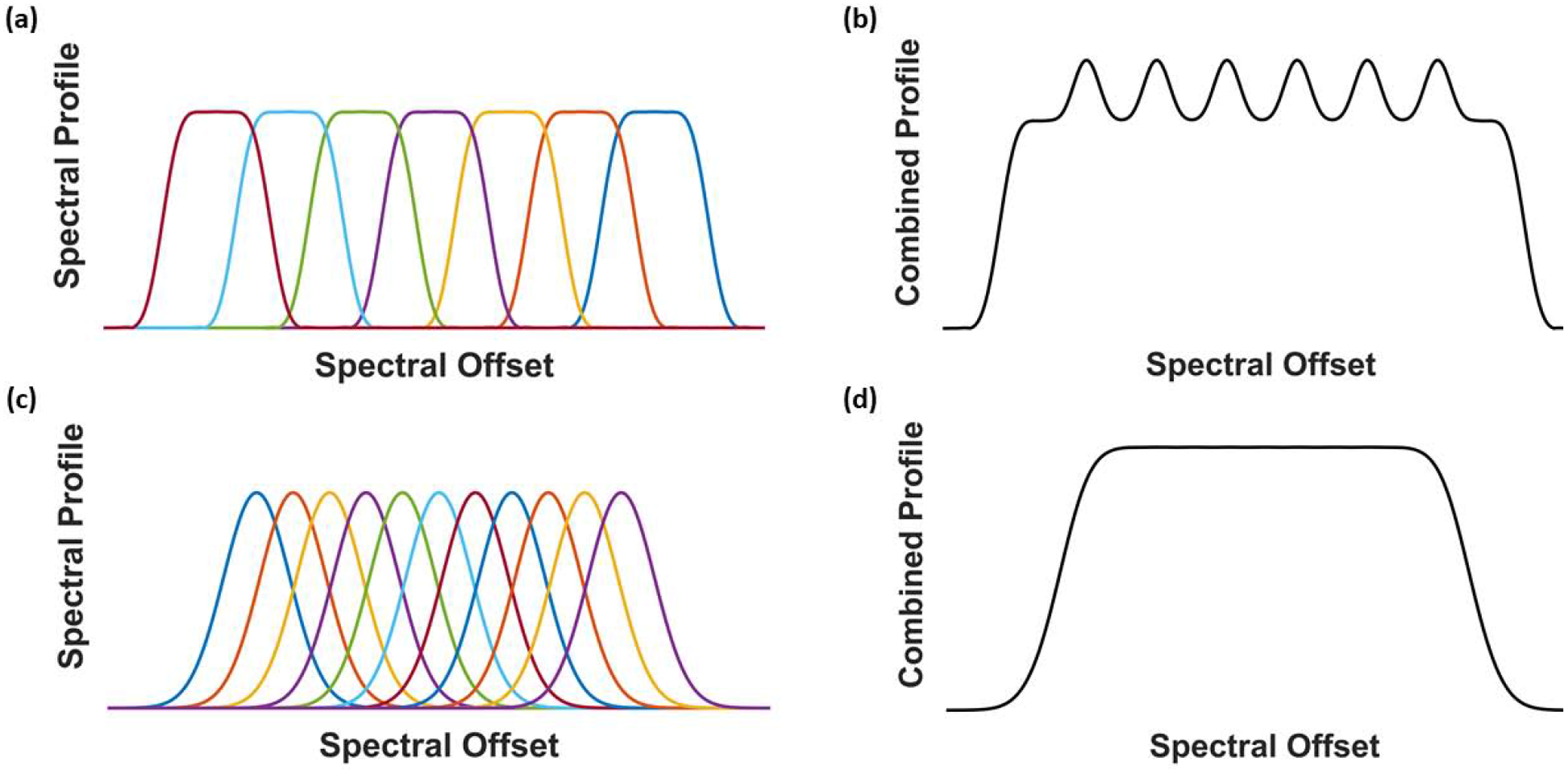
Schematic of spectral bin excitation, refocusing, and combination in multispectral imaging methods. (a) Boxcar excitation and refocusing of individual spectral bins. (b) The sum-of-squares bin combination for boxcar excitation and refocusing, yielding dramatic intensity artifacts at the bin boundaries. (c) Boxcar excitation with Gaussian refocusing pulses. (d) The sum-of-squares bin combination for Gaussian refocused pulses, with unnoticeable intensity artifact at the bin boundaries.
The second technique for imaging near metallic implants is Slice Encoding for Metal Artifact Correction (SEMAC) [61], a 3D slab-selective spin-echo sequence with VAT which uses a limited amount of phase encoding in the slab direction to image the distorted slab profile in 3D. With a set of such slabs, a complete, composite undistorted 3D image is reconstructed with knowledge of the center position of each 3D slab acquisition. With spatial selection, SEMAC images can be acquired rapidly relative to MAVRIC. However, SEMAC does not use smooth slice profiles, thereby exhibiting an image intensity artifact at slice boundaries which MAVRIC avoids with Gaussian-shaped spectral profiles.
A MAVRIC-SEMAC hybrid [62, 63] has been introduced which combines the benefits of both MAVRIC and SEMAC. The sequence, named MAVIRC-SL, is a 3D slab-selective FSE sequence. Boxcar excitation profiles are used with Gaussian refocusing, as in MAVRIC, but each pulse is spatially selective and the slab profile is imaged with a small number of phase encoding steps and view angle tilting, as in SEMAC. A persistent issue with MAVRIC-SL is high SAR due to the large bandwidth covered and the FSE-type sequence. To partially alleviate the high SAR, low refocusing flip angles (135°) are used.
4.2.4. Alternatives to Conventional Spin-Echo Imaging
An appealing alternative to both gradient-echo and spin-echo sequences is Missing Pulse Steady-State Free Precession (MPSSFP) [64–66]. MPSSFP applies a train of n RF pulses, all separated by time τ, followed by an acquisition at the position of what would have been the n+1 pulse - see Fig. 13 for a sequence diagram. At the temporal position (n + 1)τ, there is a superposition of a large number of spin and stimulated echoes, as can be seen in the extended phase graph formalism [67–69]. Kobayashi et al. explicitly calculated the extended phase graph for MPSSFP with n = 4 pulses [70, 71], providing a graphical realization of the echo formation mechanism.
Figure 13:
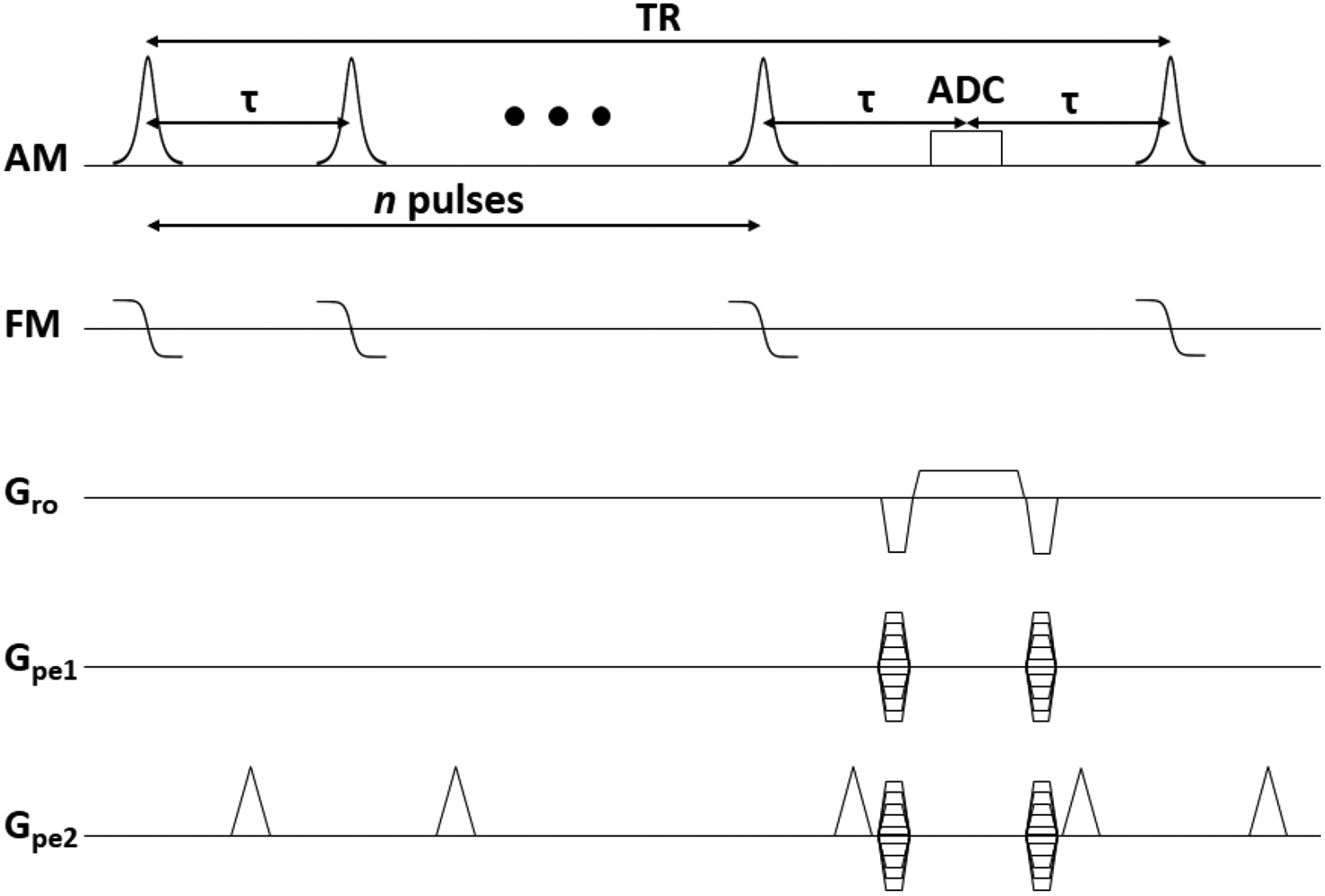
Sequence diagram for the 3D Missing Pulse Steady-State Free Precession sequence.
Using small flip angle pulses, MPSSFP is a fast, low peak RF amplitude, low SAR alternative to conventional spin echo when large pulse bandwidths are necessary. Typical repetition times are on the order of 10 – 20 ms, with an interpulse separation τ of roughly 4 – 6 ms. Moreover, MPSSFP is easily amenable to view-angle-tilting [57, 58] when using slice selective pulses. In the presence of large field inhomogeneity, high receiver bandwidth is still necessary to minimize distortion in the frequency-encoded dimension of MPSSFP.
Phantom results for 3D MPSSFP are shown in Fig. 14 as a comparison to a standard, vendor-supplied FSE sequence. While MPSSFP has visibly lower SNR, the acquisition time is approximately 14 minutes compared to the 52 minute FSE acquisition. The SNR and contrast of MPSSFP is sensitive to relaxation times, pulse separation, and pulse phase cycling, which could be used to maximize image quality for tissues of interest.
Figure 14:
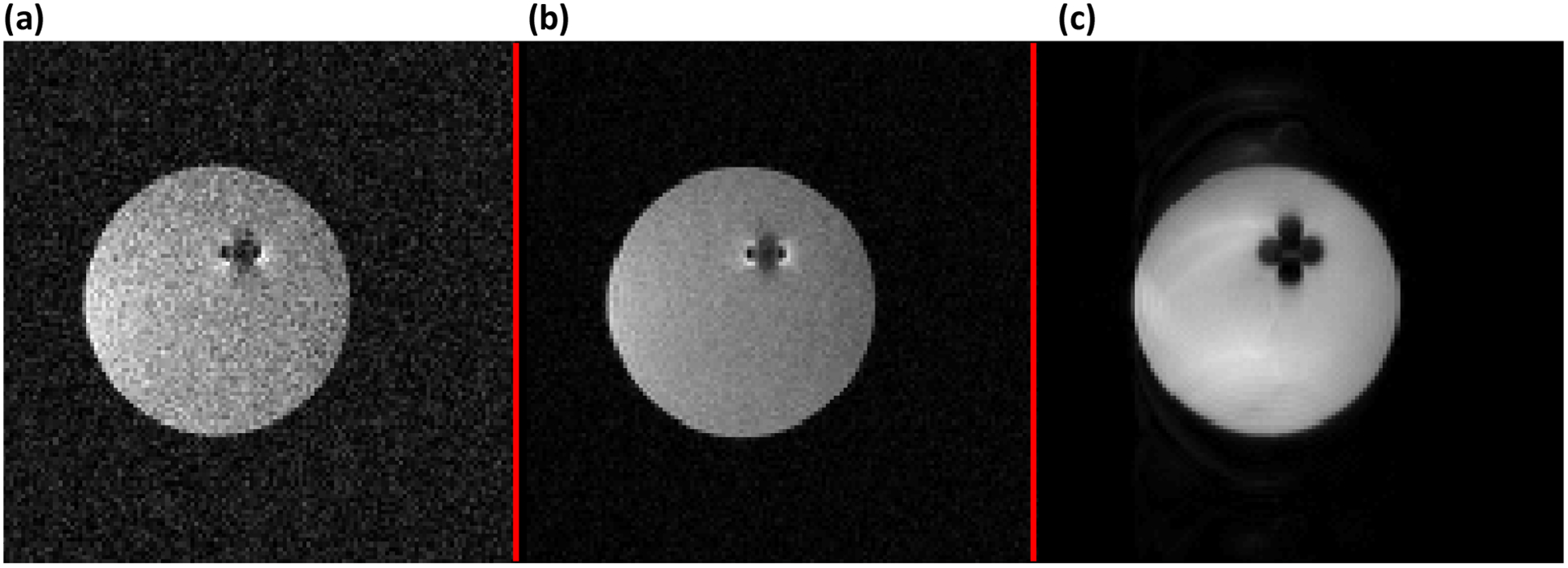
Comparison of MPSSFP to conventional fast spin-echo (FSE). All images were acquired with 2 mm isotropic resolution and FOV = 256 × 256 × 256 mm3. The pulses used for MPSSFP were 500 μs hyperbolic secant pulses with 20 kHz bandwidth and 10° flip angle. (a) MPSSFP acquired with n = 3 pulses, TR = 25.86 ms, and 250 kHz receiver bandwidth with 1 average. (b) MPSSFP image acquired with the same sequence as in (a), but with 4 averages, so that the total imaging time was approximately the same as in (c). (c) Conventional FSE with 2.25 kHz bandwidth pulses and TR = 3.07 s. Narrowband RF pulses were necessary to keep the peak RF amplitude within amplifier limits.
4.2.5. Reverse Encoding
Another promising technique for imaging with large field inhomogeneity is reverse encoding [34, 35, 72, 73], originally proposed by Chang & Fitzpatrick. In functional MRI (fMRI), reverse encoding is commonly used to reduce the strong influence of field inhomogeneity on EPI and consists of two EPI acquisitions which traverse the phase-encoded dimension of k-space in opposite directions. As the image distortions due to a spatially varying B0 field can be incorporated into a model-based reconstruction, the two acquisitions in this approach are used to find a self-consistent B0 map which registers the two distorted images to each other. Similarly, two acquisitions can be measured with opposite frequency-encoding gradients [37, 72] and correcting the image distortions in preprocessing by determining the most likely ΔB0 which registers the two images to each other. Reverse encoding demonstrates the ability not only to design imaging sequences which limit distortions, but also to correct residual distortions without direct knowledge of ΔB0.
Past techniques [74, 75] have used reverse encoding with multispectral spin-echo imaging methods or with single-, narrow-band RF pulses [72] in spin-echo sequences, as originally proposed for using reverse encoding near metallic implants. While the distortions are only along the frequency encoded direction for both images, registering 1D lines of the two images in reverse encoding to each other does not provide a physically realistic ΔB0 map, as Maxwell’s equations [76] require a non-divergent magnetic field. Hence, ΔB0 depends on the local field in 3D, not in 1D. To circumvent this issue without rigorous application of Maxwell’s equations, Skare & Andersson [72] utilized 3D B-splines to enforce a spatially continuous ΔB0 map when registering the two images from reverse-encoded MRI to each other. An alternative method involving a multiscale ΔB0 determination by convolution with various Gaussians is also possible [73]. Once an estimate of the ΔB0 map is determined, the final image is reconstructed in a method similar to [35, 44]. There, the (vectorized) distorted magnitude images f+ and f− (with ± denoting gradient polarity) are related to the “true” (vectorized) image ρ through an interpolation kernel, K+ and K−, by
| (27) |
Given N = NxNyNz voxels in each image, then f+ and f− are both N × 1 vectors, K+ and K− both are N × N, and ρ is N × 1. Estimates of K+ and K− are determined from the ΔB0 map, such that an estimate of ρ, denoted , can be found as the least-squares solution of Eq. (27). An example explicit formula for K+ and K− is given in Eq. (30). Unfortunately, the interpolation matrices K+ and K− are impractically large for 3D acquisitions. However, K+ and K− are block diagonal, as each frequency-encoded column fi, +, fi, − of the images f+, f− are distorted independently of other frequency-encoded columns. Taking x to be the frequency-encoded direction,
| (28) |
so that
| (29) |
Above, is then 2Nx × Nx, a much more manageable size.
All frequency-encoded columns of the true image can then be reconstructed independently as the least squares solution to Eq. (29), where each reconstruction requires only a small amount of computer memory [42] compared to the problem posed by Eq. (27). Construction of the Ki, + and Ki, − matrices depends on the choice of interpolation model: linear, cubic spline, sinc, etc. Denoting the true image coordinates x in the frequency-encoded direction and the distorted coordinates x′i, + and x′i, − calculated from Eq. (19), both in units of voxels, the mnth elements of Ki, + and Ki, − are constructed as
| (30) |
A key assumption in reverse encoding is that the mapping from distorted image coordinates to undistorted coordinates is injective (one-to-one) [37], a critique of which is that it is not guaranteed to be true globally [77] near metallic objects in MRI. Breaking of this assumption requires strong intrinsic field gradients, which are limited in spatial extent to be very near the implant itself. However, while implants have strong, nonlinear field gradients over short distances, the inhomogeneity field gradients due to the magnet itself are much weaker. The gradients in the latter case are smoothly varying in space, lacking the sharp transitions in resonance frequency found near metallic implants. Hence, while this assumption may break down in regions extremely close to metallic objects, it is unlikely to occur generally.
5. Available Image Contrasts
Given the available imaging sequences above, a natural question is to consider what image contrasts are available. Gradient-echo sequences with short TR, short TE, and low flip angles have historically been used for T1 weighting (e.g. FLASH [78, 79]). MPSSFP, with appropriate choice of RF phase cycling and flip angle, can offer both T1 and T2 weighting, along with diffusion weighting [71]. Unfortunately, there is not yet an option to achieve T2* weighting with large magnetic field inhomogeneity. The challenge with T2* weighting lies in the underlying contrast mechanism: local susceptibility fluctuations causing intravoxel dephasing, which becomes more visible with longer echo times in gradient-echo sequences. Large background field variations cause the signal from a voxel to decay rapidly even with modest echo times. Hence, signal is lost due to spins dephasing in the magnet’s field long before sample-induced dephasing is visible.
6. Concluding Remarks
Herein, we have presented the theoretical foundations for performing MRI in the presence of large field inhomogeneities, with particular attention given to low SAR sequences, e.g. gradient echo and MPSSFP. One conclusion is that slice distortion and an inability to adequately refocus magnetization in slices motivates the use of 3D sequences with non-selective RF pulses. When slice selection is absolutely necessary, high bandwidth RF pulses reduces slice distortion for a given slice thickness. When using a sequence with a frequency-encoded readout, image distortion can be decreased by increasing the receiver bandwidth at the expense of decreased SNR. The problem of echo shifting in GRE sequences due to field inhomogeneity can be mitigated by acquiring with increased spatial resolution and with shorter echo time.
Due to years of experience with high magnetic fields, the authors’ chosen avenue toward future compact MRI scanners hopes to exploit the many advantages and past technical developments in high field MRI. Interestingly, the progression to higher and higher magnetic field strengths over past decades has been accompanied by improved methods to correct (shim) field imperfections of magnets. Due to the availability of relatively uniform B0 at high field, use of advanced pulse sequences, such as EPI that has major advantages in terms of speed of acquisition, can be exploited and are nowadays heavily relied upon for important types of imaging, including functional (fMRI) and diffusion weighted imaging. These factors make the transition to MRI scanners with inhomogeneous B0 even less appealing. Obviously, the images acquired in a compact, high-field magnet may never reach the same quality as that obtainable with a highly homogeneous B0, but it can be argued that the latter is not essential, particularly for point-of-care (e.g. bedside) imaging. Given time and effort, the remaining hurdles to widely deploying compact high-field MRI scanners to remote locations throughout the world can be solved. The methods described herein are just the tip of the iceberg of what is expected to come.
Highlights.
Low-cost, portable MRI promises to improve access to high quality imaging worldwide
Small magnets have several thousand ppm field inhomogeneity to overcome
Imaging in high-field portable systems is achievable with proper sequence choice
Practical aspects of imaging with large field inhomogeneity are reviewed
7. Acknowledgements
This work was supported by the National Institutes of Health grants U01 EB025153 and P41 EB015894.
9. Glossary
- AM
Amplitude-modulated
- EPI
Echo-planar imaging
- FFT
Fast Fourier transform
- FLASH
Fast low-angle sho
- FM
Frequency-modulated
- fMRI
Functional magnetic resonance imaging
- FOV
Field-of-view
- FSE
Fast spin-echo
- FT
Fourier transform
- GESEPI
Gradient-echo slice excitation profile imaging
- GRE
Gradient recalled echo
- HTS
High-temperature superconductor
- kHz
Kilo-Hertz
- MAVRIC
Multi-acquisition variable-resonance image combination
- MAVIRC-SL
Multi-acquisition variable-resonance image combination selective
- MDEFT
Modified Driven Equilibrium Fourier Transform
- MHz
Mega-Hertz
- mm
Millimeters
- MPSSFP
Missing Pulse Steady-State Free Precession
- MRI
Magnetic resonance imaging
- mT
MilliTesla
- ppm
Parts per million
- RARE
Rapid acquisition with relaxation enhancement
- RF
Radiofrequency
- ROI
Region-of-interest
- SAR
Specific absorption rate
- SEMAC
Slice Encoding for Metal Artifact Correction
- SNR
Signal-to-noise ratio
- SPI
Single-Point Imaging
- SPRITE
Single-Point Ramped Imaging with T1 Enhancement
- STRAFI
Stray Field Imaging
- sw
Spectral width
- T
Tesla
- TBP
Time-bandwidth product
- TE
Echo time
- TR
Repetition time
- VAT
View-angle tilting
Footnotes
Publisher's Disclaimer: This is a PDF file of an unedited manuscript that has been accepted for publication. As a service to our customers we are providing this early version of the manuscript. The manuscript will undergo copyediting, typesetting, and review of the resulting proof before it is published in its final form. Please note that during the production process errors may be discovered which could affect the content, and all legal disclaimers that apply to the journal pertain.
Declaration of interests
The authors declare that they have no known competing financial interests or personal relationships that could have appeared to influence the work reported in this paper.
8. References
- [1].Ogbole GI, Adeyomoye AO, Badu-Peprah A, Mensah Y, Nzeh DA, Survey of magnetic resonance imaging availability in West Africa, Pan Afr Med J, 30 (2018) 240. [DOI] [PMC free article] [PubMed] [Google Scholar]
- [2].OECD (2020), Magnetic resonance imaging (MRI) units (indicator). doi: 10.1787/1a72e7d1-en (Accessed on 14 July 2020). [DOI] [Google Scholar]
- [3].Cooley CZ, Haskell MW, Cauley SF, Sappo C, Lapierre CD, Ha CG, Stockmann JP, Wald LL, Design of sparse Halbach magnet arrays for portable MRI using a genetic algorithm, IEEE Trans Magn, 54 (2018). [DOI] [PMC free article] [PubMed] [Google Scholar]
- [4].Cooley CZ, Stockmann JP, Armstrong BD, Sarracanie M, Lev MH, Rosen MS, Wald LL, Two-dimensional imaging in a lightweight portable MRI scanner without gradient coils, Magn Reson Med, 73 (2015) 872–883. [DOI] [PMC free article] [PubMed] [Google Scholar]
- [5].McDaniel PC, Cooley CZ, Stockmann JP, Wald LL, The MR Cap: A single-sided MRI system designed for potential point-of-care limited field-of-view brain imaging, Magn Reson Med, 82 (2019) 1946–1960. [DOI] [PMC free article] [PubMed] [Google Scholar]
- [6].Huang ZHRLMWLJSSY, Magnet array for a portable magnetic resonance imaging system in: 2015 IEEE MTT-S 2015 International Microwave Workshop Series on RF and Wireless Technologies for Biomedical and Healthcare Applications (IMWS-BIO), IEEE, 2015, pp. 92–95. [Google Scholar]
- [7].Ren ZH, Mu WC, Huang SY, Design and Optimization of a Ring-Pair Permanent Magnet Array for Head Imaging in a Low-Field Portable MRI System, IEEE Transactions on Magnetics, 55 (2019) 1–8. [Google Scholar]
- [8].O’Reilly T, Teeuwisse WM, Webb AG, Three-dimensional MRI in a homogenous 27cm diameter bore Halbach array magnet, J Magn Reson, 307 (2019) 106578. [DOI] [PubMed] [Google Scholar]
- [9].McDonald PJ, Newling B, Stray field magnetic resonance imaging, Reports on Progress in Physics, 61 (1998) 1441–1493. [Google Scholar]
- [10].Blümich B, Blümler P, Eidmann G, Guthausen A, Haken R, Schmitz U, Saito K, Zimmer G, The NMR-mouse: construction, excitation, and applications, Magnetic Resonance Imaging, 16 (1998) 479–484. [DOI] [PubMed] [Google Scholar]
- [11].Guthausen G, Guthausen A, Balibanu F, Eymael R, Hailu K, Schmitz U, Blumich B, Soft-matter analysis by the NMR-MOUSE, Macromol Mater Eng, 276 (2000) 25–37. [Google Scholar]
- [12].Macovski A, Conolly S, Novel approaches to low-cost MRI, Magn Reson Med, 30 (1993) 221–230. [DOI] [PubMed] [Google Scholar]
- [13].Morgan P, Conolly S, Scott G, Macovski A, A readout magnet for prepolarized MRI, Magn Reson Med, 36 (1996) 527–536. [DOI] [PubMed] [Google Scholar]
- [14].Venook RD, Matter NI, Ramachandran M, Ungersma SE, Gold GE, Giori NJ, Macovski A, Scott GC, Conolly SM, Prepolarized magnetic resonance imaging around metal orthopedic implants, Magn Reson Med, 56 (2006) 177–186. [DOI] [PubMed] [Google Scholar]
- [15].Balibanu F, Hailu K, Eymael R, Demco DE, Blumich B, Nuclear magnetic resonance in inhomogeneous magnetic fields, J Magn Reson, 145 (2000) 246–258. [DOI] [PubMed] [Google Scholar]
- [16].Halbach K, Design of permanent multipole magnets with oriented rare earth cobalt material, Nuclear Instruments and Methods, 169 (1980) 1–10. [Google Scholar]
- [17].Raich H, Blümler P, Design and construction of a dipolar Halbach array with a homogeneous field from identical bar magnets: NMR Mandhalas, Concepts in Magnetic Resonance Part B: Magnetic Resonance Engineering, 23B (2004) 16–25. [Google Scholar]
- [18].Soltner H, Blümler P, Dipolar Halbach magnet stacks made from identically shaped permanent magnets for magnetic resonance, Concepts in Magnetic Resonance Part A, 36A (2010) 211–222. [Google Scholar]
- [19].Windt CW, Soltner H, van Dusschoten D, Blumler P, A portable Halbach magnet that can be opened and closed without force: the NMR-CUFF, J Magn Reson, 208 (2011) 27–33. [DOI] [PubMed] [Google Scholar]
- [20].Aubert G, Permanent magnet for nuclear magnetic resonance imaging equipment, in, US, 1994.
- [21].Marques JP, Simonis FFJ, Webb AG, Low-field MRI: An MR physics perspective, J Magn Reson Imaging, 49 (2019) 1528–1542. [DOI] [PMC free article] [PubMed] [Google Scholar]
- [22].Hennig J, Nauerth A, Friedburg H, RARE imaging: a fast imaging method for clinical MR, Magn Reson Med, 3 (1986) 823–833. [DOI] [PubMed] [Google Scholar]
- [23].Sarracanie M, LaPierre CD, Salameh N, Waddington DEJ, Witzel T, Rosen MS, Low-Cost High-Performance MRI, Sci Rep, 5 (2015) 15177. [DOI] [PMC free article] [PubMed] [Google Scholar]
- [24].Parkinson B, Development of a Highly Compact 1.5 T Functional MRI System with Minimal Infrastructural Requirements, in: Proceedings of the 26th Annual Meeting of ISMRM, Paris, France, 2018. [Google Scholar]
- [25].Parkinson B, Magnets: Design, Manufacturing, Installation, Present & Future Technology, in: Proceedings of the 26th Annual Meeting of ISMRM, Paris, France, 2018. [Google Scholar]
- [26].Garwood M, DelaBarre L, The return of the frequency sweep: designing adiabatic pulses for contemporary NMR, J Magn Reson, 153 (2001) 155–177. [DOI] [PubMed] [Google Scholar]
- [27].Tannús A, Garwood M, Adiabatic pulses, NMR in Biomedicine, 10 (1997) 423–434. [DOI] [PubMed] [Google Scholar]
- [28].Pauly J, Nishimura D, Macovski A, A k-space analysis of small-tip-angle excitation, Journal of Magnetic Resonance (1969), 81 (1989) 43–56. [DOI] [PubMed] [Google Scholar]
- [29].Brown RW, Cheng Y-CN, Haacke EM, Thompson MR, Venkatesan R, Magnetic Resonance Imaging, 2014.
- [30].Nishimura DG, Principles of Magnetic Resonance Imaging, 2010.
- [31].Stehling MK, Turner R, Mansfield P, Echo-planar imaging: magnetic resonance imaging in a fraction of a second, Science, 254 (1991) 43–50. [DOI] [PubMed] [Google Scholar]
- [32].Haacke EM, The effects of finite sampling in spin-echo or field-echo magnetic resonance imaging, Magn Reson Med, 4 (1987) 407–421. [DOI] [PubMed] [Google Scholar]
- [33].Mugler III JP, Brookeman JR, The optimum data sampling period for maximum signal-to-noise ratio in MR imaging, Rev. Magn. Reson. Med, 3 (1988) 1–51. [Google Scholar]
- [34].Andersson JL, Skare S, A model-based method for retrospective correction of geometric distortions in diffusion-weighted EPI, Neuroimage, 16 (2002) 177–199. [DOI] [PubMed] [Google Scholar]
- [35].Andersson JLR, Skare S, Ashburner J, How to correct susceptibility distortions in spin-echo echo-planar images: application to diffusion tensor imaging, NeuroImage, 20 (2003) 870–888. [DOI] [PubMed] [Google Scholar]
- [36].Reichenbach JR, Venkatesan R, Yablonskiy DA, Thompson MR, Lai S, Haacke EM, Theory and Application of Static Field Inhomogeneity Effects in Gradient-Echo Imaging, Journal of Magnetic Resonance Imaging, 7 (1997) 266–279. [DOI] [PubMed] [Google Scholar]
- [37].Chang H, Fitzpatrick JM, A technique for accurate magnetic resonance imaging in the presence of field inhomogeneities, IEEE Trans Med Imaging, 11 (1992) 319–329. [DOI] [PubMed] [Google Scholar]
- [38].Shepp LA, Logan BF, The Fourier reconstruction of a head section, IEEE Transactions on Nuclear Science, 21 (1974) 21–43. [Google Scholar]
- [39].Macovski A, Noise in MRI, Magn Reson Med, 36 (1996) 494–497. [DOI] [PubMed] [Google Scholar]
- [40].Schneider E, Glover G, Rapid in vivo proton shimming, Magn Reson Med, 18 (1991) 335–347. [DOI] [PubMed] [Google Scholar]
- [41].Glover GH, Gullberg GT, Magnet Shimming Technique Using Information Derived from Chemical Shift Imaging, in, 1988.
- [42].Weis J, Budinský L.u., Simulation of the influence of magnetic field inhomogeneity and distortion correction in MR imaging, Magnetic Resonance Imaging, 8 (1990) 483–489. [DOI] [PubMed] [Google Scholar]
- [43].Jezzard P, Balaban RS, Correction for geometric distortion in echo planar images from B0 field variations, Magn Reson Med, 34 (1995) 65–73. [DOI] [PubMed] [Google Scholar]
- [44].Munger P, Crelier GR, Peters TM, Pike GB, An inverse problem approach to the correction of distortion in EPI images, IEEE Trans Med Imaging, 19 (2000) 681–689. [DOI] [PubMed] [Google Scholar]
- [45].Yang QX, Williams GD, Demeure RJ, Mosher TJ, Smith MB, Removal of local field gradient artifacts in T2*-weighted images at high fields by gradient-echo slice excitation profile imaging, Magn Reson Med, 39 (1998) 402–409. [DOI] [PubMed] [Google Scholar]
- [46].Young IR, Cox IJ, Bryant DJ, Bydder GM, The benefits of increasing spatial resolution as a means of reducing artifacts due to field inhomogeneities, Magnetic Resonance Imaging, 6 (1988) 585–590. [DOI] [PubMed] [Google Scholar]
- [47].Jezzard P, Attard JJ, Carpenter TA, Hall LD, Nuclear magnetic resonance imaging in the solid state, Progress in Nuclear Magnetic Resonance Spectroscopy, 23 (1991) 1–41. [Google Scholar]
- [48].Gravina S, Cory DG, Sensitivity and Resolution of Constant-Time Imaging, Journal of Magnetic Resonance, Series B, 104 (1994) 53–61. [Google Scholar]
- [49].Halse M, Goodyear DJ, MacMillan B, Szomolanyi P, Matheson D, Balcom BJ, Centric scan SPRITE magnetic resonance imaging, J Magn Reson, 165 (2003) 219–229. [DOI] [PubMed] [Google Scholar]
- [50].Balcom BJ, Macgregor RP, Beyea SD, Green DP, Armstrong RL, Bremner TW, Single-Point Ramped Imaging with T1 Enhancement (SPRITE), J Magn Reson A, 123 (1996) 131–134. [DOI] [PubMed] [Google Scholar]
- [51].Demas V, Sakellariou D, Meriles CA, Han S, Reimer J, Pines A, Three-dimensional phase-encoded chemical shift MRI in the presence of inhomogeneous fields, Proc Natl Acad Sci U S A, 101 (2004) 8845–8847. [DOI] [PMC free article] [PubMed] [Google Scholar]
- [52].Mullen M, Kobayashi N, Garwood M, Two-dimensional frequency-swept pulse with resilience to both B1 and B0 inhomogeneity, J Magn Reson, 299 (2019) 93–100. [DOI] [PMC free article] [PubMed] [Google Scholar]
- [53].Roemer PB, Edelstein WA, Hayes CE, Souza SP, Mueller OM, The NMR phased array, Magn Reson Med, 16 (1990) 192–225. [DOI] [PubMed] [Google Scholar]
- [54].Constantinides CD, Atalar E, McVeigh ER, Signal-to-noise measurements in magnitude images from NMR phased arrays, Magn Reson Med, 38 (1997) 852–857. [DOI] [PMC free article] [PubMed] [Google Scholar]
- [55].Henkelman RM, Measurement of signal intensities in the presence of noise in MR images, Med Phys, 12 (1985) 232–233. [DOI] [PubMed] [Google Scholar]
- [56].Epstein CL, Magland J, A novel technique for imaging with inhomogeneous fields, J Magn Reson, 183 (2006) 183–192. [DOI] [PMC free article] [PubMed] [Google Scholar]
- [57].Cho ZH, Kim DJ, Kim YK, Total inhomogeneity correction including chemical shifts and susceptibility by view angle tilting, Med Phys, 15 (1988) 7–11. [DOI] [PubMed] [Google Scholar]
- [58].Butts K, Pauly JM, Gold GE, Reduction of blurring in view angle tilting MRI, Magn Reson Med, 53 (2005) 418–424. [DOI] [PubMed] [Google Scholar]
- [59].Ugurbil K, Garwood M, Ellermann J, Hendrich K, Hinke R, Hu XP, Kim SG, Menon R, Merkle H, Ogawa S, Salmi R, Imaging at High Magnetic-Fields - Initial Experiences at 4-T, Magn Reson Quart, 9 (1993) 259–277. [PubMed] [Google Scholar]
- [60].Koch KM, Lorbiecki JE, Hinks RS, King KF, A multispectral three-dimensional acquisition technique for imaging near metal implants, Magn Reson Med, 61 (2009) 381–390. [DOI] [PubMed] [Google Scholar]
- [61].Lu W, Pauly KB, Gold GE, Pauly JM, Hargreaves BA, SEMAC: Slice Encoding for Metal Artifact Correction in MRI, Magn Reson Med, 62 (2009) 66–76. [DOI] [PMC free article] [PubMed] [Google Scholar]
- [62].Koch KM, Brau AC, Chen W, Gold GE, Hargreaves BA, Koff M, McKinnon GC, Potter HG, King KF, Imaging near metal with a MAVRIC-SEMAC hybrid, Magn Reson Med, 65 (2011) 71–82. [DOI] [PubMed] [Google Scholar]
- [63].Gutierrez LB, Do BH, Gold GE, Hargreaves BA, Koch KM, Worters PW, Stevens KJ, MR imaging near metallic implants using MAVRIC SL: initial clinical experience at 3T, Acad Radiol, 22 (2015) 370–379. [DOI] [PMC free article] [PubMed] [Google Scholar]
- [64].Patz S, Wong ST, Roos MS, Missing pulse steady-state free precession, Magn Reson Med, 10 (1989) 194–209. [DOI] [PubMed] [Google Scholar]
- [65].Dreher W, Erhard P, Leibfritz D, Fast three-dimensional proton spectroscopic imaging of the human brain at 3 T by combining spectroscopic missing pulse steady-state free precession and echo planar spectroscopic imaging, Magn Reson Med, 66 (2011) 1518–1525. [DOI] [PubMed] [Google Scholar]
- [66].Hwang KP, Flask C, Lewin JS, Duerk JL, Selective missing pulse steady state free precession (MPSSFP): inner volume and chemical shift selective imaging in a steady state sequence, J Magn Reson Imaging, 19 (2004) 124–132. [DOI] [PubMed] [Google Scholar]
- [67].Weigel M, Extended phase graphs: dephasing, RF pulses, and echoes - pure and simple, J Magn Reson Imaging, 41 (2015) 266–295. [DOI] [PubMed] [Google Scholar]
- [68].Hennig J, Multiecho imaging sequences with low refocusing flip angles, Journal of Magnetic Resonance (1969), 78 (1988) 397–407. [Google Scholar]
- [69].Kaiser R, Bartholdi E, Ernst RR, Diffusion and field-gradient effects in NMR Fourier spectroscopy, The Journal of Chemical Physics, 60 (1974) 2966–2979. [Google Scholar]
- [70].Kobayashi N, Idiyatullin D, Garwood M. U.S. Patent 10,591,566 (2020).
- [71].Kobayashi N, Parkinson B, Idiyatullin D, Adriany G, Theilenberg S, Juchem C, Garwood M, Development and Validation of 3D MP-SSFP to Enable MRI in Inhomogeneous Magnetic Fields, Magn Reson Med, in press (2020). [DOI] [PMC free article] [PubMed] [Google Scholar]
- [72].Skare S, Andersson JL, Correction of MR image distortions induced by metallic objects using a 3D cubic B-spline basis set: application to stereotactic surgical planning, Magn Reson Med, 54 (2005) 169–181. [DOI] [PubMed] [Google Scholar]
- [73].Holland D, Kuperman JM, Dale AM, Efficient correction of inhomogeneous static magnetic field-induced distortion in Echo Planar Imaging, Neuroimage, 50 (2010) 175–183. [DOI] [PMC free article] [PubMed] [Google Scholar]
- [74].Shi X, Quist B, Hargreaves B, Pile-up and ripple artifact correction near metallic implants by alternating gradients, in: Proceedings of the 25th Annual Meeting of ISMRM, Honolulu, HI, USA, 2017, pp. 574. [Google Scholar]
- [75].Kwon K, Kim D, Kim B, Park H, Unsupervised learning of a deep neural network for metal artifact correction using dual-polarity readout gradients, Magn Reson Med, 83 (2020) 124–138. [DOI] [PubMed] [Google Scholar]
- [76].Jackson JD, Classical Electrodynamics, 3 ed., John Wiley & Sons, Inc., 1999. [Google Scholar]
- [77].Koch KM, Hargreaves BA, Pauly KB, Chen W, Gold GE, King KF, Magnetic resonance imaging near metal implants, J Magn Reson Imaging, 32 (2010) 773–787. [DOI] [PubMed] [Google Scholar]
- [78].Haase A, Frahm J, Matthaei D, Hanicke W, Merboldt KD, FLASH imaging. Rapid NMR imaging using low flip-angle pulses, Journal of Magnetic Resonance (1969), 67 (1986) 258–266. [DOI] [PubMed] [Google Scholar]
- [79].Waugh JS, Sensitivity in Fourier transform NMR spectroscopy of slowly relaxing systems, Journal of Molecular Spectroscopy, 35 (1970) 298–305. [Google Scholar]