Understanding the spatio‐temporal pattern of COVID‐19 outbreak in India using GIS and India's response in managing the pandemic

Abstract

Due to the outbreak of Coronavirus, humans all over the world are facing several health problems. The present study has explored the spatio‐temporal pattern of Coronavirus spread in India including spatial clustering, identification of hotspot, spatial heterogeneity, and homogeneity, spatial trend, and direction of COVID‐19 cases using spatial statistical analysis during the period of 30 January to 20 June 2020. Besides, the polynomial regression model has been used for predictions of COVID‐19 affected population and related deaths. The study found positive spatial heterogeneity in COVID‐19 cases in India. The study has also identified 17 epicentres across the country with high incidence rates. The directional distribution of ellipse polygon shows that the spread of COVID‐19 now trending towards the east but the concentration of cases is mainly in the western part of the country. The country's trend of COVID‐19 follows a fourth‐order polynomial growth and is characterized by an increasing trend. The prediction results show that as on 14 October India will reach 14,660,400 COVID‐19 cases and the death toll will cross 152,945. Therefore, a “space‐specific” policy strategy would be a more suitable strategy for reducing the spatial spread of the virus in India. Moreover, the study has broadly found out seven sectors, where the Government of India lacks in terms of confronting the ongoing pandemic. The study has also recommended some appropriate policies which would be immensely useful for the administration to initiate strategic planning.

1. INTRODUCTION

The novel Coronavirus‐2019 disease¹ has posed an incredible danger to all mankind throughout the world (Mondal & Ghosh, 2020; Nadeem, 2020). It is a contagious human disease and its fast pace of infection and rate of transmission among people has introduced a new challenge for the health care system (Clara‐Rahola, 2020). The average incubation period of COVID‐19 is 5 to 6 days, although it can take up to 2 to 14 days for appearing symptoms (Arti, 2020; Pandey, Chaudhary, Gupta, & Pal, 2020) and during this long incubation period, the COVID‐19 infected patients can transmit the virus without any symptoms to his/her surrounding people (Koubaa, 2020). An interesting fact comes in light that the spread of the virus is following the geographic pattern, such as northern Italy is more affected than the southern part, and cities are more affected than rural areas. Currently, more than 70 percent of the total COVID‐19 cases across the world are reported from 11 countries namely the US, Brazil, India, Russia, South Africa, Peru, Mexico, Colombia, Chile, Spain and Iran. The World Health Organization (WHO) has reported that more than 213 countries and territories around the world are affected by the spreading of this deadly virus through direct contact by the affected people. However, the extent of the casualty rate is quite different for various land areas and essentially differs considering the demography of population and health care facilities (Ranjan, 2020) as well as on the effective steps taken by the government from time to time (Bedford et al., 2020).

In addition, Chowell and Rothenberg (2018) mentioned that infectious diseases (respiratory influenza, pneumonia, respiratory syncytial virus; vector‐borne like malaria, dengue, and Zika; sexually transmitted disease such as HIV and syphilis) follow a dynamic spatial pattern along with the associated socio‐economic and environmental conditions. Hence, COVID‐19, as an infectious disease, it has a high probability that it would follow a spatial pattern. In India, Ghosh, Dinda, Chatterjee, Das, and Mahata (2019) found that the spatial clustering of dengue follows a particular spatial trend in the city of Kharagpur. Similar kind of findings has been found by Rasam et al. (2014) in an exploratory analysis of the cholera spatial pattern in the district of Sabah in Malaysia. It has also been found that infectious disease also follows a general spatial pattern and cluster based on the infected person or locations (Lessler, Salje, Grabowski, & Cummings, 2016). Brockmann, David, and Gallardo (2009) mentioned that infectious diseases are strongly correlated with human mobility in the globalized world. Therefore, it also has a probability that COVID‐19 would follow a spatial trend according to human mobility in a country. Moreover, it was also found that in the case of COVID‐19, the distance has played a significant role to spread. Akhtar, Kraemer, and Gardner (2019) has shown that the Zika epidemic (infectious disease) in South America shows a spatial pattern with an overall accuracy of above 85 percent. Stresman et al. (2018) have found that hotspots of malaria, spread the disease in the surrounding areas following a systematic pattern. Inter household contact plays an agency role in malaria spreading. In India, it has been reported that cities are mainly playing the COVID‐19 epicentre, which indicates a systematic spatial pattern (Kaur et al., 2020).

Moreover, these infectious diseases have rapidly increased over the last two decades. The unhygienic environmental condition is responsible for the increasing rate of infectious diseases. For example, the waterborne diseases in the city of Tamil Nadu in summer seasons are identified with the dirty water from open sewage lines and drains, which show the clear linear pattern of disease spread. In the case of COVID‐19, it has been found that it spreads through social contacts with the active facilitation of illegal animal markets in Wuhan, China (Adnan, Khan, Kazmi, Bashir, & Siddique, 2020; Zhu et al., 2020).

However, there is a growing understanding that infectious diseases have specific geography; therefore, it is becoming increasingly important to study the different layers of health‐related data for a particular place. The geographic information systems (GIS) prepares a perfect base to merge explicit data regarding the disease and their interpretation in connection with population habitancy, encompassing health and social services and the natural environment (Zhou et al., 2020). However, a spatial examination of the epidemic focused on the question “Where is the disease concentrating and in which direction is it spreading?” GIS is being used in the epidemic studies to find where people are affected the most and the also makes it possible to view disease distributions in great detail. Haining (2012) mentioned that GIS plays a significant role to determine the trend of any disease spread over space. Moreover, the Tobler’s “first law of geography, explains that everything is related to everything else, but near things are more related than distant things. The spatial autocorrelation has critically explained this phenomenon and it is widely applicable in case of spatial spread of COVID‐19 in any country.

Therefore, in context of COVID‐19 spread in India, the present study aims to explore the spatial pattern of COVID‐19 outbreak including estimation of hotspots, clustering, spatial direction, and heterogeneity with the help of GIS in different time frames. Besides, the temporal trend of COVID‐19 cases in India has also been explored and predictions of positive cases have been estimated. In addition to that India’s response in managing the pandemic and necessary suitable policy dimensions also has been discussed in this study.

The rest of the paper has been organized as follows: Section 2 elaboratesthe method of this study, where different method and data sources have discussed. In Section 3, the results of the above‐mentioned research have been discussed. We have discussed the result according to each method applied in this study. Section 4 concludes, where the major findings have explained, in addition the selected suggest measure to confronting the COVID‐19 has highlighted.

2. METHODOLOGY AND DATA SOURCES

2.1. Hot‐Spot Analysis

As mentioned earlier, the present paper focuses on hotspots identification, spatial autocorrelation, and spatio‐temporal mapping of COVID‐19 spread in India. For hotspot analysis of present COVID‐19 in India Getis–Ord Gi* statistics have been calculated. It is a distance‐based z‐score value that tells where the particular phenomena significantly cluster. A high z‐score and small p‐value for a feature indicate a significant hot spot (Ruktanonchai, Pindolia, Striley, Odedina, & Cottler, 2014). The near‐zero z‐score indicates no spatial clustering. Following is the statistical expression of Getis–Ord Gi*:

$$G_I^{*}=\frac{{\sum }_{j=1}^n{w}_{i,j}{x}_j-\overline{X}{\sum }_{j=1}^n{w}_{\mathit{ij}}}{\sqrt[S]{\frac{\left[n{\sum }_{j=1}^n{w}_{i,j}^2-{\left({\sum }_{j=1}^n{w}_{i,j}\right)}^2\right]}{n-1}}},$$

where, x _j is the attribute value for feature j, w _i,j is the spatial weight between i and j; n is the total number of features. $\overline{X}$ represents the mean whereas s denotes the standard deviation.

2.2. Spatial association

To understand the spatial autocorrelation, Moran’s I‐ method has been applied, which provides a correlation measure to a spatial context. The Moran’s I index value would indicate how the COVID‐19 affected cases are spatially distributed and what kind of pattern is being followed, namely, random(I = 0), dispersed(I < 0), and clustered(0 < I) (Chen, 2013). Following is the statistical expression of Moran’s I:

$$I_W=\frac{N{\sum }_{i=1}^n{\sum }_{i=1}^n{W}_{\mathit{ij}}\left(x_i-\overline{x}\right)\left(x_j-\overline{x}\right)}{\left({\sum }_{i=1}^n{\sum }_{i=1}^n{W}_{\mathit{ij}}\right){\sum }_{i=1}^n{\left(x_i-\overline{x}\right)}^2},$$

where N is the number of observation (in the present study i.e. polygon), $\overline{x}$ is the mean of the variable, x _i is the value of the variable in a particular location, w _ij is the weight indexing location of i and j.

The inverse distance weighted (IDW) technique has been applied to compute the spatio‐temporal pattern analysis of COVID‐19 spread and distribution. The IDW generates an average value of COVID‐19 spread for unsampled locations across India using values from nearby weighted locations. The larger the power coefficient, the stronger is the weight of nearby points. The following equation estimates the value z at an unsampled location j:

$$Z_p=\frac{{\sum }_{i=1}^n\left(\frac{z_i}{d_i}\right)}{{\sum }_{i=1}^n\frac{1}{d_i^p}},$$

where the sigma simply means the number of points that will be interpolated. A smaller number in the denominator (more distance) has less effect on the interpolated (Z_p) value. In the IDW, the sampled points and values are superimposed on top and an interpolated raster is generated within the boundary. This results in nearby points having a greater influence on the unsampled locations.

In addition, the geographically weighted regression (GWR 1) has applied to understand the spatial prediction of diseases based on other demographic variables. In the present study, the GWR analytical framework is following:

$$y_{\mathit{dcc}=}{\beta }_{0\left(u_i,v_i\right)}+{\beta }_1{T}_{p\left(u_i,v_i\right)}+{\beta }_2{P}_{d\left(u_i,v_i\right)}+{\beta }_3{H}_{i\left(u_i,v_i\right)}+{\beta }_4{S}_{C\left(u_i,v_i\right)+}{\beta }_5{P}_{\mathit{hc}\left(u_i,v_i\right)}+{\beta }_6{C}_{\mathit{hc}\left(u_i,v_i\right)}+{\epsilon }_I,$$

where ${\beta }_{0\left(u_i,v_i\right)}$ is the geographical co‐ordinate of the point i. T _p is the total population, P _d is the population density, H _i is the health infrastructure, S _c is the sub centre, P _hc is the primary health centre, and C _hc is the community health centre of the ith district. The regression coefficient is estimated at each data location. In GWR, an observation is weighted following its proximity to location i, so that the weighting of observation is no longer constant. The weight of each point is calculated as:

$$\widehat{\beta }\left(u_i,v_i\right)=(x^{t}w(\left(u_i,v_i\right)x^{-1}{x}^{t}w\left(u_i,v_i\right)y.$$

In GWR, the weight assigned to each observation is based on a distance decay function centred on observation i. In GWR, the local weights matrix is calculated from a kernel function W that places more weight on locations that are closer in space to the calibration location than those that are more distant in space.

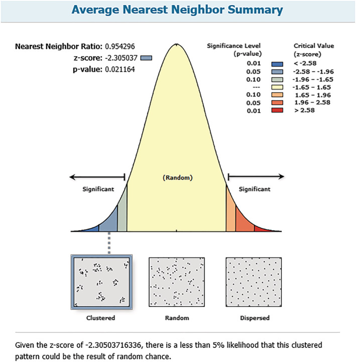
2.3. Average nearest neighbour (ANN)

The widely applied ANN technique of clustering has been used to determine the spatial clustering of COVID‐19 trends in India. It considers the distance between each feature centroid and its nearest neighbour’s centroid location. If the average distance is less than the average for a hypothetical random distribution, the distribution of the features being analysed is considered clustered otherwise features are considered dispersed (Ebdon, 1985). The following are details of the average nearest neighbour ratio:

$$\mathit{ANN}=\frac{{\overline{D}}_O}{{\overline{D}}_E},$$

where, ${\overline{D}}_O$ is the observed mean distance between each feature and its nearest neighbour:

$${\overline{D}}_O=\frac{{\sum }_{i=1}^n{d}_i}{n},$$

and ${\overline{D}}_E$ is the expected mean distance for the feature given in a random pattern:

$${\overline{D}}_E=\frac{0.5}{\sqrt{\frac{n}{A}}},$$

where n is the total number of features, A is the area of minimum enclosing rectangle around the feature. The average ANN’s z score statistics calculated as:

$$z=\frac{{\overline{D}}_O-{\overline{D}}_E}{\mathit{SE}},$$

where, standard error $\left(\mathit{SE}\right)=\frac{0.26136}{\sqrt{\frac{n^2}{A}}}.$

If the index (average nearest neighbour ratio) is less than 1, the pattern exhibits clustering. If the index is greater than 1, the trend is towards dispersion.

2.4. Directional distribution (standard deviational ellipse)

The standard deviational ellipses show the spatial characteristics of COVID‐19 dispersion and directional trends. It is based on either Euclidean or Manhattan distance. The standard deviation ellipse is the most widely used technique to predict a disease outbreak over time. The standard deviational ellipse is given as:

$${\mathit{SDE}}_x=\sqrt{\frac{{\sum }_{i=1}^n{\left(x_i-\overline{x}\right)}^2}{n}},$$

$${\mathit{SDE}}_Y=\sqrt{\sum _{i=1}^n{\left(y_i-\overline{y}\right)}^2},$$

where x and y are the co‐ordinates for feature i, { $\overline{x}$, ӯ} represent the mean centre for the features, and n is equal to the total number of features.

2.5. Temporal trend analysis

For understanding the future trend of the total affected cases of COVID‐19 in India, the polynomial regression model has been applied. The model predicts the prevalence of COVID‐19 in India given the time‐series data. The polynomial regression is based on the curvilinear relationship between a dependent and an independent variable. The following is the statistical expression of a polynomial regression model:

$$y_c={\beta }_0+{\beta }_{1}X+{\beta }_2{X}^2+{\beta }_3{X}^3+{\beta }_4{X}^4=\sum _{j=0}^M{w}_j{x}^j,$$

where X is the independent variable and M is the order of the polynomial. β ₀ is the bias and also the intercept, β _1, β _2, β _3, β _4, are the weight or partial coefficients assigned to the predictors and n is the degree of the polynomial. The future value of COVID‐19 affected cases has been estimated based on 80 days of observation and estimated values are validated and corrected through the root mean squared log error (RMSLE) method considering ten days’ actual data. The formula of RMSLE is:

$$\mathit{\text{RMSLE}}=\sqrt{\frac{1}{n}}{\sum }_{i=1}^n\left(\mathit{log}(y_i+1\right)-({\widehat{y+1)}}^2,$$

where, $y_i\mathit{\text{and}}\widehat{y}$ are the actual and predicted values respectively. The statistical uncertainty of the predicted value has been estimated based on the 95 percent predicted interval.

2.6. Data sources

The district and state‐level COVID‐19 cases data have been collected from the official website of the Ministry of Health and Family Welfare. For country‐level time‐series data, the situational reports from WHO have been used. The time‐series data has been collected from 30 January to 20 June 2020; which include total confirmed, recovered, and death cases of COVID‐19 in India by the states and union government in India. Besides, the high resolution (30” × 30” or approximately 1 km) LandScan‐2018 population data has been used for GWR analysis. However, as a lesser number of populations has been tested compare to total population in India. therefore, there is a limitation of the database.

3. RESULT AND DISCUSSION

3.1. Spatiotemporal pattern of COVID‐19 hotspots and outliers

A commendable spatio‐temporal pattern all over the world can be identified by spatially analysing a statistically viable and important clustering of the locale through the hotspot and the cold‐spots. The hotspots analysis revealed that core clustering of high COVID‐19 affected districts are clustered mostly in the western regions (as of 20 June analysis) and variously encompassed by 60 districts (Maharashtra and Gujarat) though initially (as of 21 March 2020) the spread of various COVID‐19 clusters was along the southern (Tamil Nadu‐Chennai, Andhra Pradesh‐Hyderabad, Karnataka‐Bengaluru, and Kerala), western (Maharashtra‐Mumbai, Gujarat‐ Ahmedabad; two main commercial hubs of the country) and north‐central (Delhi‐ the national capital) regions of the country and encompassed 139 districts (Figure 1a). This result clearly portrays a high amount of incidence rate in the area. Similarly, a significant cold spots clusters were visible in the Eastern region (as of 21 March analysis) comprising Assam, West Bengal, Bihar and their surrounding regions encompassed 262 districts (Figure 1a) and the increase in the number of cases with respect to time in the eastern region has led to the sharp decline of cold spots that existed previously in that region. As of 21May, and 20 June, the cold spot areas in the eastern part disappeared completely (Figure 1c and d) indicating that the next phase of virus spread could possibly target these zones. Even at the pick of the pandemic stage in India, comparatively lower numbers of cases were reported from the east, except for a few centres situated at Gangetic West Bengal, Coastal Odisha, and along the Ganga valley of eastern Uttar Pradesh and Bihar. The hot spots analysis during the peak of lockdown phase (21 April) indicates intense clustering of high values around Maharashtra, Gujarat, and Rajasthan (Figure 1b); however, the initial high values clustering around Kerala, Karnataka, Tamil Nadu diminished in this phase possibly due to pre‐emptive actions taken by the Kerala, Karnataka, Tamil Nadu state governments and union government’s policies. Except for most likely hotspots and cold spots, other areas were identified as secondary categories, among which most areas do not show significant spatio‐temporal trends as shown in Figure 1. With time the yellow zones expanded covering larger areas because the cold spot zones turned into yellow due to the jump in the new COVID‐19 cases. West Bengal, Bihar, Assam, Chhattisgarh, Odisha, Jharkhand, Tripura, Nagaland are the states where the trend is very high (Figure 1d). However, in north‐east India, the numbers of COVID‐19 cases are much lower as compared to the rest of the country. It is because none of the airports in this region is internationally connected; a few numbers of immigrants have come to this region and out of them, most are travellers. From another point of view, after analysing hotspots, four places have been spotted (Delhi, Mumbai, Chennai, and Kolkata) which came out to be significant hotspots and they gradually extended the infection to the neighbouring locale. These cities are one of the heavily populated regions of the nation and pulled in an enormous number of floating populations from various parts of the nation, which made these places to be largely affected by COVID‐19. On the other hand, airports of these cities are internationally connected and acted as penetration paths of COVID‐19 from foreign countries. Figure 2 shows the standard deviation of COVID‐19 cases across the country, where a high Z‐score value corresponding to high amount of incidence rate in the area.

FIGURE 1.

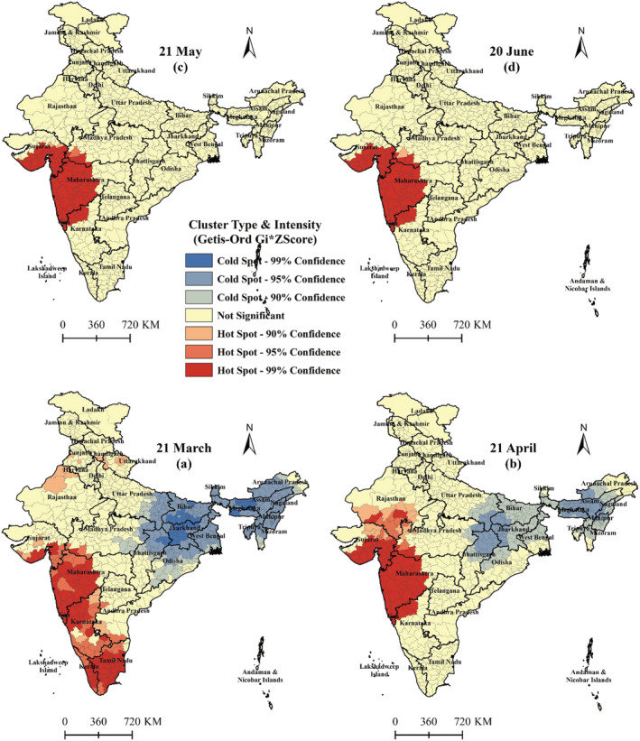
Pattern and intensity of COVID‐19 hotspots in India (red and blue colours area represents statistically significant hotspots and cold‐spots respectively)

FIGURE 2.

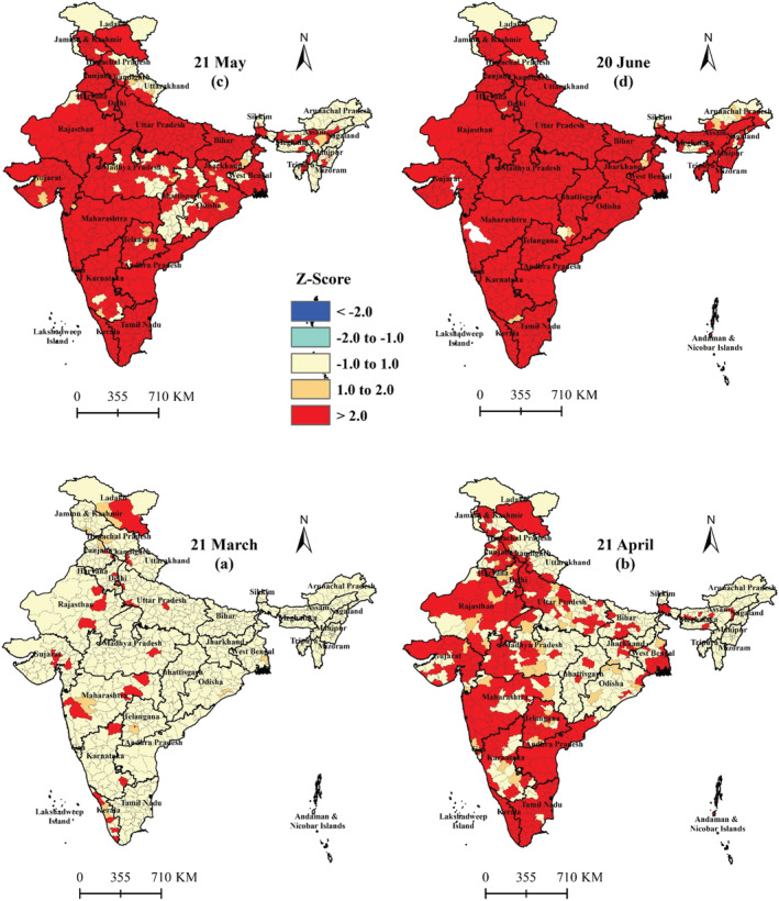
Z‐score mapping for symbolizing standard deviation of COVID‐19 cases across the country (red colours area indicates Z‐score above 2 standard deviation)

3.2. Spatial association and GIS interpolation mapping

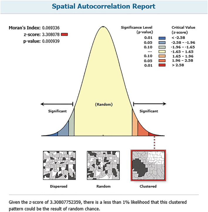
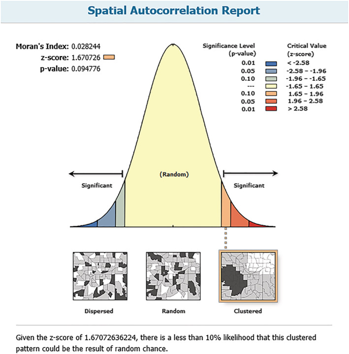
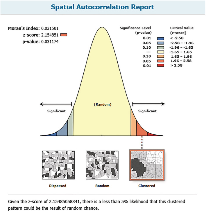
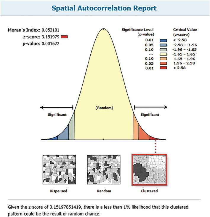
The Moran’s I based spatial autocorrelation values represent that there is a positive spatial auto correlation in COVID‐19 cases throughout India. The Moran’s I value for 21 March COVID‐19 cases was recorded 0.069 (p = 0.0009), and the Z‐score was 4.67 (Figure A1), which shows the data is statistically significant and confirms the presence of spatial structure. While the Moran’s I value for 21 April was 0.028 (p = 0.09) indicating a heterogeneity structure of COVID‐19 growth across the country (Figure A2). However, the Moran’s I value on 21 May was recorded 0.031, p = 0.031 (Figure A3) and on 20 June it was 0.053, p = 0.001 (Figure A4), showing an increasing trend of Moran’s I values which indicates that the structure of COVID19 growth across the country will reach a homogenous spatial structure. Besides, there was a significant temporal variation in the spatial dependence of COVID‐19 cases including early dates followed by a general size and significance of Moran’s I (range‐1 to +1) from 0.069 on 21 March to 0.053 on 20 June 2020.

Figure 3, shows the general intensification and spatio‐temporal spread of the COVID‐19 pandemic in India. In the first phase, (as of 21 March) possible potential outreach was mostly around south Delhi (northern region), Mumbai (Western region), Hyderabad, Bangalore (Southern region) and Indore (Central region), Kerala (Southern region), Ladakh (Northern region) and Bhilwara (Western region). With time, epicentre expanded and newly emerged around the South Delhi, Agra in the Northern region; Mumbai, Thane, Pune, Surat, Ahmedabad Jaipur, Jodhpur in the Western region; Chennai, Hyderabad, Kurnool in the Southern region, Bhopal, Indore in the central region; Lucknow, Kanpur central in North‐eastern region; and Kolkata and its surrounding areas in the eastern region (Figure 3b). Kerala played a major role in the second phase analysis, by showing a marked improvement. This scenario continued into the next phases (21 May) as well and rapid growth and expansion were observed around the Mumbai, Ahmedabad, Indore, Chennai, Kolkata, and surrounding areas (Figure 3c). However, in the last phase (as of 20 June), most of the areas has recorded total cases in the triple digit. The gravity of the COVID‐19 cases is very high in the Western regions of the country especially Maharashtra and Gujarat. The existent epicentres are significantly affected its surrounding areas. Besides the virus spread significantly in the north‐eastern regions especially in the eastern districts of West Bengal, Bihar, Jharkhand, Assam, and gradually these areas come under pandemic situations due to inter‐state in migration of migrant labour from Western and Southern parts of the country (Figure 3d). Therefore, the eastern part of the country now faces an imminent threat of becoming epicentres of COVID‐19 cases and in the near future most probably these areas will become major hotspots as the spread of the virus in western regions may start to peak or gradually decline. This analysis showed a variety in the spatial dispersion of COVID‐19 cases in the nation and cases are expanding day by day.

FIGURE 3.

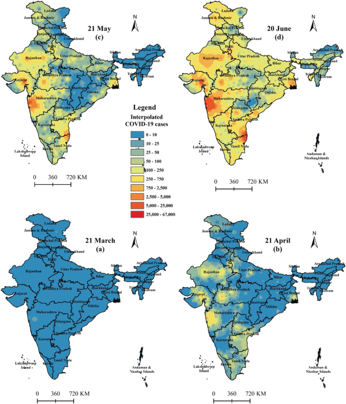
Spatio‐temporal trend of COVID‐19 outbreak in India (continuous surfaces produced by interpolating district wise COVID‐19 cases)

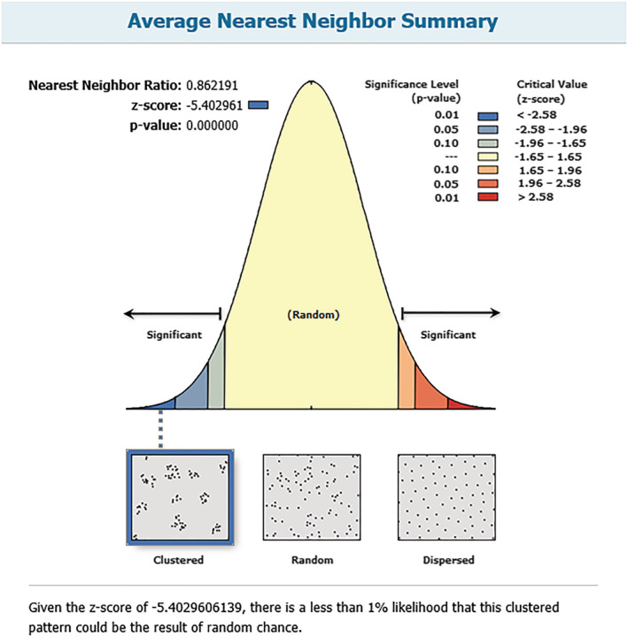
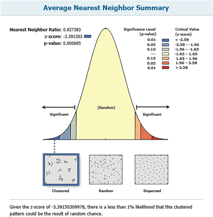
Further, the spatial distribution pattern of COVID‐19 cases was examined by ANN analysis provides the average distance from each point to another within its closest vicinity. The result of ANN shows the nearest neighbour ratio (R), Z‐score, and P values. If the ANN ratio <1, the case pattern is clustered; otherwise, it is dispersed. Similarly, a higher Z‐value indicates a higher degree of a cluster. As of 21 March, the average nearest neighbour ratio was < 1(%) i.e. 0.73 (p = 0.001), it was recorded 0.86 (p = 0.001) on 21 April; 0.92 (p = 0.001) on 21 May and 0.95 (p = 0.02) on 20 June analysis (Figures A5, A6, A7 and A8 respectively); while the Z values for COVID‐19 incident were −4.06, −5.40, −3.39 and −2.30 respectively (Table 1). It means that during the assessment period the pattern of the case was clustered, though it was higher on 21^st March as compared to 20^th June.

TABLE 1.

Average nearest neighbour summary

Date	Nearest neighbour ration (NR)	Observed distance	Z‐score	P‐value
21/3/2020	0.73	85126.53	−4.61	0.000004
21/4/2020	0.86	57642.16	−5.40	0.000001
21/5/2020	0.93	52109.96	−3.39	0.000695
20/6/2020	0.95	49750.25	−2.31	0.021

Figure 4 shows the location of COVID‐19 geographic mean centres, directional distribution of COVID‐19 cases for 21 March, 21 April, 21 May, and 20 June. The spatial mean centre is the analysis of the concentration point of any geographical phenomena (Abd Majid, Muhamad Nazi, & Mohamed, 2019). It suggests that all the mean centre of COVID‐19 cases were located very close to the western part of the country with little temporal shifting. The mean centre on 2^t March was located at X co‐ordinate 20°57′2.8′′ N and Y co‐ordinate 76°39′47.31′′E (in Buldana district of Maharashtra); whereas for 21 April, it was slightly shifted (127.68 km westward) and located at X co‐ordinate 21°39′1.4′′ N and Y co‐ordinate 76°7′16′′ E (East and West Nimar districts of Madhya Pradesh). However, as of 21 May the mean centre shifted 108.40 km towards South and located at X co‐ordinate 20°40′20.47′′ N and Y co‐ordinate 76°2′4.97′′ E (in Buldana district of Maharashtra) and then again 91 km shifted towards East and located at X co‐ordinate 20°33′2.2′′ N and Y co‐ordinate 76°54′1.42′′ E (in Akola district of Maharashtra) as of 20 June. While the directional distribution of ellipse polygon indicates that initially the spread of COVID‐19 has followed North–South direction and with time it is gradually shifting towards East. Moreover, the ellipse polygon of 21 March has greater length towards North–South direction, which covered 68 percent of the distribution. The standard deviation of the distribution on the X‐axis was 1154.27 km and Y‐axis was 394.14 km, and the ratio between the X and Y axis was 2.93. Whereas, on 20 June it was 689.16 km on X‐axis and 860.98 km on Y‐axis with ratio 0.80. The direction of ellipse appeared that initially (as on 21 March) the distribution of COVID‐19 cases in India was towards North–South direction with 5°22′48″ rotation angle and with time the length of X‐axis has significantly reduced (as on 20 June length reduced by 465.11 km) and similarly Y‐axis length has increased by 466.84 km (Table 2) with rotation angle equal to 7°26′24″. This indicates that the disease is gradually spreading towards the east of the country and more probably in the next phase the direction of the pandemic will appear in the West–East direction.

FIGURE 4.

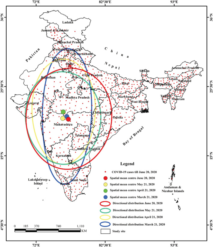
Spatial mean centre, directional distribution of COVID‐19 cases in India for 21 March, 21 April, 21 May and 20 June, 2020

TABLE 2.

Summarizes the characteristics of standard deviational ellipse of the COVID‐19 cases in India

Date	Location of mean centre		Ellipse size of the Epidemics		Orientation of the ellipse
	Mean centre (X)	Mean Centre (Y)	X std. distance (km)	Y std. distance (km)
21/3/2020	20°57′2.8′′ N	76°39′47.31′′E	1154.27	394.14	5°22′48”
21/4/2020	21°39′1.4′′ N	76°7′16′′ E	896.98	506.6	4°12′36”
21/5/2020	20°40′20.47′′ N	76°2′4.97′′ E	606.90	790.00	0°48′0”
20/6/2020	20°33′2.2′′ N	76°54′1.42′′ E	689.16	860.98	7°26′24”

The GWR model indicates that population density, the total number of the populations, health infrastructure, sub centres, primary health care (PHC) and community health centre (CHC) have explained more than 89 percent (R² = 0.89) of total variance at the country level of COVID‐19 affected cases. Moreover, Figure 5 shows the spatial pattern of R² which indicates that almost the entire south‐eastern part of the country’s COVID‐19 is explained by the selected explanatory variables. Further, the standard residuals from the GWR are spatially random (Moran’s I = − 0.07; z = 3.99; p < 0.001), implying that there are other factors which also affects the COVID‐19 affected cases in district level. The residuals map also shows that COVID‐19 affected cases are underestimated primarily in the western part of the country (Figure 5).

FIGURE 5.

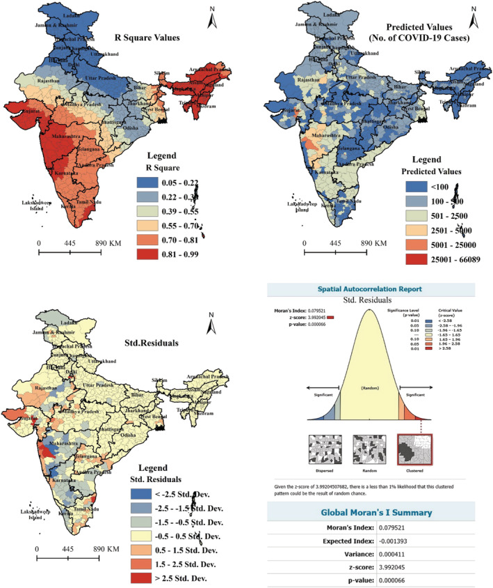
Spatial pattern of local R², predicted, and standard residuals from the GWR model of COVID‐19 affected cases (20 June, 2020)

3.3. Spatio‐temporal trend and intensification of COVID‐19 in India

Although India registered the first COVID‐19 case in the last of January 2020 in Kerala, the number of new confirmed cases in India was very less till 21 March, 2020. From the beginning of April, the number of newly confirmed cases increased rapidly. Till the study period, India registered maximum fresh positive cases on 20 June (14,516 cases) and maximum deaths for a single day was on 17 June (2003 cases). The daily cumulative and new confirmed cases from up to the 20 June 2020 are summarized in figure 6. This figure shows that the curve of cumulative positive cases left the ground in the first week of April. The gap between the ground and the curve rapidly increased day by day and the curve got steeper slope as the days passed by. After 143 days from the date of the first COVID‐19 case reported in the country, India recorded 12,948 death cases (3.27%) and 213,831 recovered (54.12%) cases (as of 20 June). Out of the total cases, 79.25 percent of the cases were reported in the last 36 days of the study period. As of 1^st April 2020, the percentage of recovered and death cases was 10.33 percent and 2.32 percent respectively. However, more than 50 percent of infected individuals (54.06%) have recovered till 20 June 2020 and the fatality rate was about 3.27 percent. Percentage of recovered enhanced by 6.37 percent in the last 20 days and an amount of casualty likewise followed a lower pattern in comparison of other infected nations, which ascribed to the update of diagnostic measures and health care service facilities for COVID‐19 in India. Figure 7 represents the trend of recovered and death cases in India for the entire period of the study.

FIGURE 6.

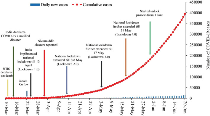
Temporal trend of reported COVID‐19 cases in India from 10 March to 20 June, 2020

FIGURE 7.

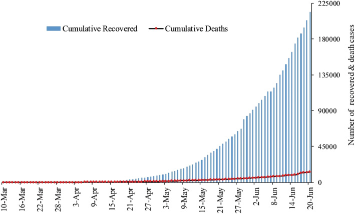
Changes in number of cumulative recovered and death in India from 10 March to 20 June, 2020

The spatial spread of COVID‐19 cases differs according to the situation of the states and districts and the geographic range of the cases has increased with each passing day. Figure 8 shows the spatial distribution of COVID‐19 cases among the districts of India from 21 March to 20 June. At the districts level, 41.94 percent cases were concentrated in six districts namely South Delhi (1,363), Ahmedabad (1,298), Pune (660), Mumbai (3029), Indore (915) and Jaipur (537) as of 21 April, however, 299 districts were not affected by COVID‐19 disease (Figure 6d). While almost 96.67 percent districts are affected by COVID‐19 disease as on 20 June and more than 50 percent cases are concentrated in seven districts namely South Delhi (34,840), Ahmedabad (18,837), Pune (15,881), Mumbai (66,484), Indore (915) and Chennai (39,470), which clearly shows an uneven distribution across the country. Whereas in the state level, till 6 April three states reported more than 500 cases (Maharashtra‐748, Delhi‐523, Tamilnadu‐517), while on 29 April twelve states registered more than 500 cases (Andhra Pradesh‐1,259, Delhi‐3,314, Gujarat‐3,744, Maharashtra‐9,318, Madhya Pradesh‐2,387, Rajasthan‐2,364, Uttar Pradesh‐2053, Tamil Nadu‐2058, Telengana‐1,004, West Bengal‐725, Karnataka‐523, Jammu & Kashmir‐565). However, with the passage of time, outbreak spread rapidly and fourteen new states were added namely Kerala, Odisha, Haryana, Bihar, Punjab, Ladakh, Chhattisgarh, Goa, Jharkhand, Manipur, Tripura, Uttarakhand, Assam, and Himachal Pradesh in the list of more than 500 positive cases as on 20 June. Among which 81.24 percent of COVID‐19 cases concentrated in seven states (namely Delhi−53,116, Gujarat‐ 26,141, Maharashtra‐ 124,331, Madhya Pradesh‐ 11,582, Rajasthan‐ 14,156 and Tamil Nadu‐54,449, Uttar Pradesh‐15785, West Bengal‐13,090), of which independently Maharashtra accounting 31.47 percent (one‐third) of the total cases with 45.51 percent deaths in India. On the other hand, Lakshadweep, Daman, Diu have not registered any confirmed COVID‐19 case till 20 June 2020 (Figure 9).

FIGURE 8.

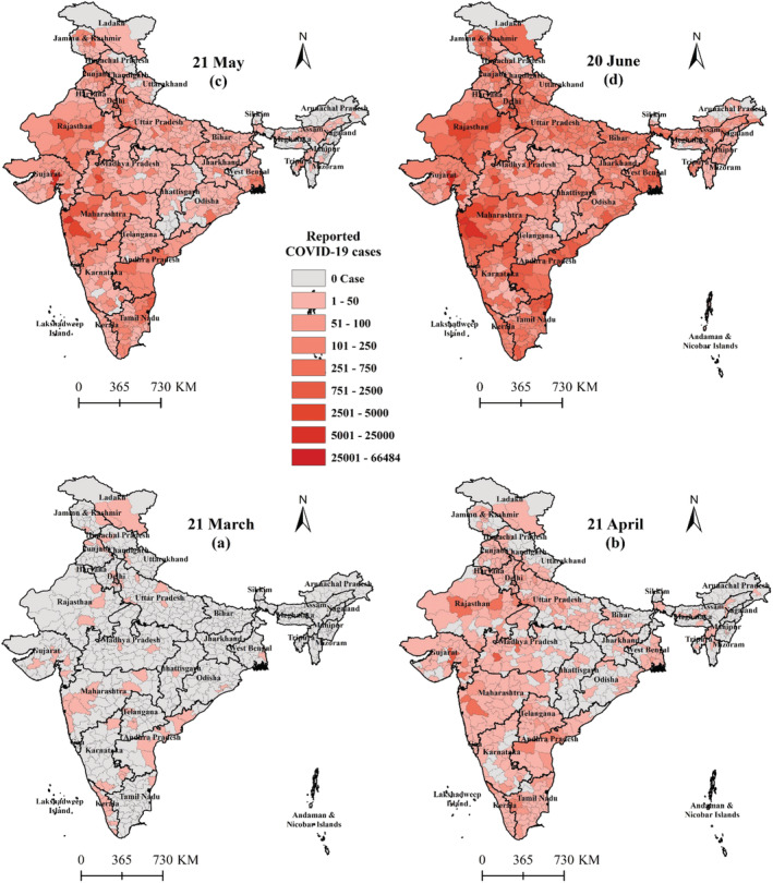
District wise spatio‐temporal variation of reported COVID‐19 cases in India (21 March to 20 June, 2020)

FIGURE 9.

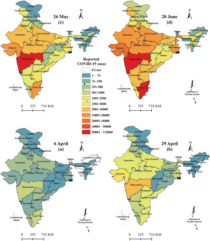
State‐wise spatio‐temporal variation of COVID‐19 cases in India (6 April to 20 June, 2020)

The spatiotemporal pattern of deaths and recovered cases in India has been shown in Figures 10 and 11 respectively. The recovered and morbidity rates of any pandemic in any area generally relies upon the procedures to fight against the circumstance just as on the regional elements, ecological conditions, financial structure, social awareness and medicinal facilities of that district. In India Kerala, Goa and Manipur are some of the states which are quite successful in preventing the rapid spread of the positive cases. On the other side, in the case of deaths, Gujarat (6.19%), Madhya Pradesh (4.27%), West Bengal (4.04%) and Maharashtra (4.74%) reported more than 4 percent fatality rate as on 20 June. However, within the study period, no death case has reported from Andaman and Nicobar Islands, Dadra and Nagar Haveli, Goa, Manipur, Mizoram, Sikkim, Nagaland and Arunachal Pradesh. On the other hand, fifteen states/UTs namely Andaman & Nicobar (77.78%), Chhattisgarh (65.63%), Meghalaya (75%), Chandigarh (82.68%), Madhya Pradesh (75.53%), Rajasthan (77.69%), Gujarat (69.49%), Himachal Pradesh (62.68%), Bihar (70.99%), Odisha (70.49%), Punjab (68.78%), UP (61.06%), Uttarakhand (65.82%), Nagaland (63.13%) and Assam (61.98%) reported more than 60 percent recovered cases. However, Ladakh (12.76%), Goa (16.28%), Mizoram (0.77%), Sikkim (7.14%), Arunachal Pradesh (10.68%), Dadra and Nagar Haveli (22.58%) reported significantly low recovered cases in India.

FIGURE 10.

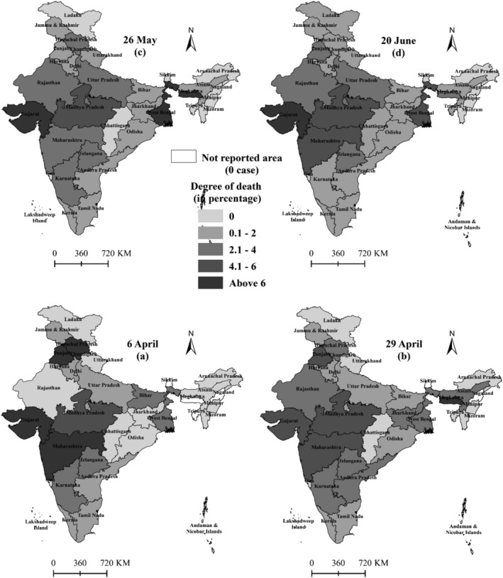
State‐wise spatio‐temporal variation of COVID‐19 death cases in India (6 April to 20 June, 2020)

FIGURE 11.

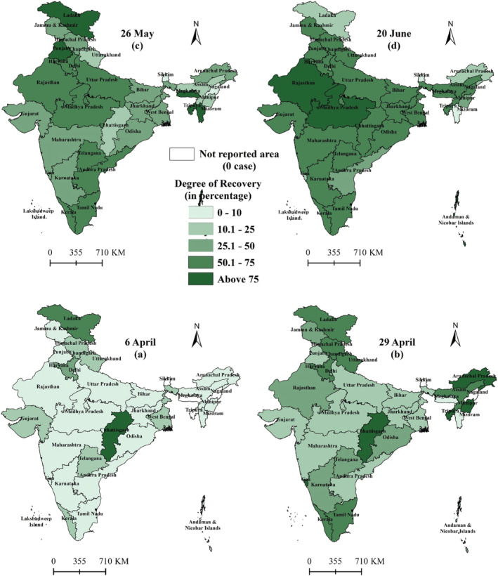
State‐wise spatio‐temporal variation of recovered cases in India (6 April to 20 June, 2020)

3.4. Regression analysis and prediction of COVID‐19 cases in India

As we are probably aware of the fact that COVID‐19 is an infectious disease with a high transmission rate (Pandey et al., 2020) and there was no significant development in the quantity of COVID‐19 cases in India before March 2020, in this manner, 80 days training data at which the disease grows and reported noteworthy deaths (from 2 April to 20 June 2020) has been utilized to investigate the future pattern of the pandemic in India. To check the validation of the model, 10 days’ actual data (21 June to 30 June 2020) has been used and root means square log error (RMSLE) has been calculated. The RMSLE for both of the predicted confirmed cases and death cases is 0.002 and 0.017 respectively (see Table A1 and A2). Table A3 shows the prediction result of the number of confirmed cases and death cases in India using the polynomial regression model. The predicted result shows that on 14 October 2020, the number of COVID‐19 cases in India will reach 14,660,400 positive cases (which are near 1.21 percent of the total population) and 152,945 death cases. Figure 12 & 13 shows the day‐wise prediction of COVID‐19 positive cases and deaths in India respectively, with the 95 percent prediction interval from 21 June to 14 October 2020.

FIGURE 12.

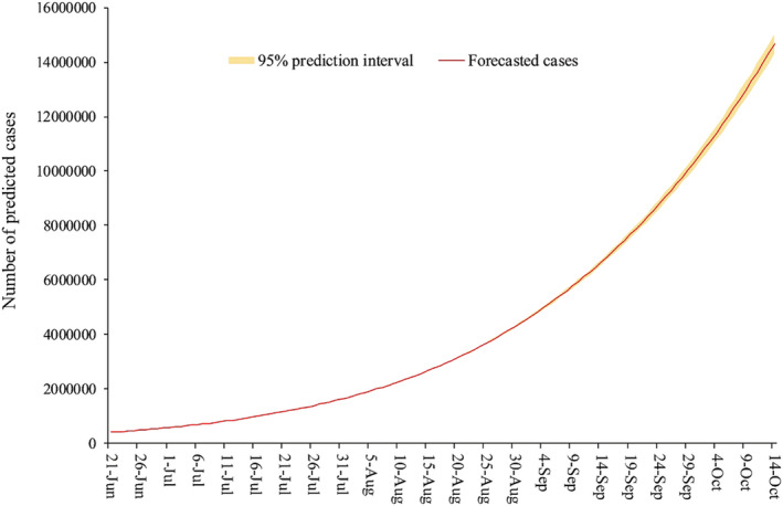
Prediction of number of COVID‐19 patients in India till 14 October, 2020 (actual values are recorded till 20 June, 2020)

FIGURE 13.

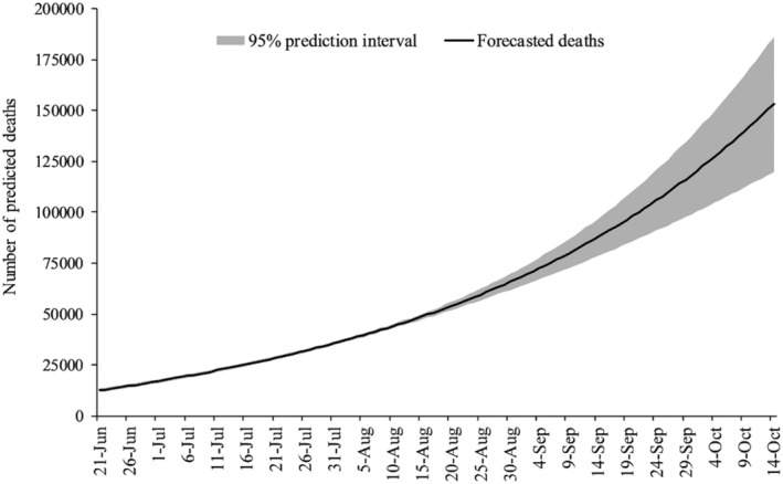
Prediction of number of deaths by COVID‐19 infection in India till 14 October, 2020 (actual values are recorded till 20 June, 2020)

3.5. India’s response to the COVID‐19 pandemic

In the last week of January 2020, China was suffering from the COVID‐19 pandemic (Li et al., 2020). On 29 January the Indian Health Ministry advised Indians not to travel to China. After confirming the first case of the country on 30 January, the Government of India (GoI) announced to screen all the travellers who came from China after 15 January. Following the second positive case, GoI decided to cancel all the e‐visa facilities for the Chinese as well as for all the foreigners who are residing in China. Observing the situation, India started preparing for its upcoming battle against this virus. However, in this study, India’s response of the COVID‐19 pandemic was divided into two‐part, the first part will discuss the positive measures taken in India; the second part will focus on the lack of policy design to confront the COVID‐19 pandemic.

The government along with other institutions began to spread social awareness among the target population through the distribution of pamphlets, mass SMS and media. The Ministry of Foreign Affairs, India had suspended all the visas on or before 3 March to the nationals of Italy, Iran, South Korea, and Japan after confirming the confirmed cases of 21 Italian tourists along with their Indian bus driver, conductor and tourist guide (The Hindu, 4 March 2020). Observing the growing confirmed cases, the GoI officially decided not to celebrate the Holi 2 festival to avoid the gatherings and it was a message to all the residents of the country to be aware of the outbreak of COVID‐19. To contain the human to human transmission the government declared shut all the schools and colleges till 31 March in the state. On 13 March 2020, the Indian government imposed a strict travel restriction and suspended gatherings of 200 people and essentially closed its international and regional borders. The visas were revoked refuting entry to all except selective foreigners.

Moreover, based on WHO guidelines, mandatory thermal screening was setup at air and seaports for all passengers. Following the rapid growth rate of positive cases, shopping malls, theatres, and educational institutions were closed. On the other hand, all religious gatherings and festivals were also banned in India. The National Restaurant Association of India (NRAI) issued an advisory to all its members to shut down their restaurants from 18 to 31 March, 2020.

However, on 19 March, India calls for social distancing and appealed for “Janata Curfew” on 22 March (The Hindu, 20 March 2020). Day after the “Janata Curfew” GoI announced to stop all the domestic flights till the end of March to contain the inter‐state transmission. On the evening of 24 March, GoI announced a nationwide lockdown for 21 days till 14 April. It was the first phase of lockdown to contain the outbreak of this deadly virus in the country. According to reports from the Union Health Ministry of India, the death toll rose to 339, with 10,363 cases overall till 14 April, the last day of lockdown. On the same day observing the rapid growth of COVID‐19 positive cases, GoI extended the lockdown period till 3 May as the second phase of it, that is, “Lockdown 2.0”. During this lockdown period government strictly restricted outward movement of population from the containment zone except for maintaining essential services (including medical emergency) and stopped all vehicular movement, public transport, and personnel movement across the country. All the district headquarters provided helpline numbers for the preventive measures required and the need for prompt reporting to health facilities, availability of essential services, and administrative orders. Keeping in view of the growing number of positive cases, GoI extended “Lockdown 3.0” till 17 May followed by “Lockdown 4.0” up to 31 May. The WHO praised India’s COVID‐19 national lockdown as “tough and timely.” The Ministry of Health and Family Welfare (MoHFW), Government of India identified 123 hotspot districts with large outbreaks on 15 April 2020 based on reported cases and directed the concerned state governments to follow the similar way of identification of hotspots in state level and repeat this exercise every week for implementing strict containment measures. In addition, government‐designated red, orange and green zones considering multiple factors taking into consideration the number of cases, doubling rate, the extension of testing and surveillance feedback to classify the districts (Figure 14). The districts will be labelled as green zone if there are no confirmed cases since the last 21 days. Whereas, the red zones or hotspot districts are defined after taking into account the total number of active cases, doubling rate of confirmed cases, the extent of testing, and surveillance feedback, while rest of the districts that are neither defined as red or green will be considered as the orange zone. In green zones, government permitted all activities except the limited number of activities that are banned throughout the country irrespective of the zones. However, buses can function with up to 50 percent seating capacity. These benevolent precautionary measures mainly played a significant role to contain the pandemic in India compared to other affected countries worldwide.

FIGURE 14.

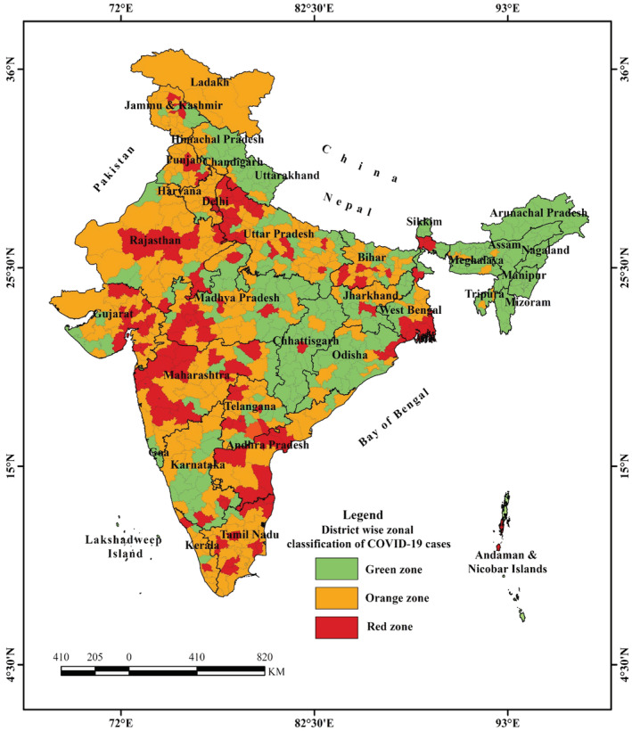
District wise zone classification of COVID‐19 cases in India (The Union Health Ministry on first May, 2020 listed 130 districts in red zone, 284 in the orange zone and 319 in the green zone for a week after 3 May, 2020)

Further, after imposing the lockdown, the GoI announced a relief package of Rs 1.7 lakh crore. These included five kilograms of wheat or rice and one kilogram of pulses to each low‐income family, free cooking gas cylinders to 83 million poor families, one‐time cash transfers of $13.31–$30 to senior citizens and $6.65 per month to the poor women through Jandhan's account and medical insurance of $66,000 to all the frontline doctors, nurses and paramedics to the sanitary workers (World economic forum, 2020).

However, apart from the above positive measures, there are many shortcomings of the government's response to confront the COVID‐19 Pandemic. The GoI has been facing criticism in different angles from the experts. Here, the study also points out the lacuna of India’s measures in combating the COVID‐19 Pandemic.

First, in spite of the primary warning from the WHO in January, 2020, the Indian government showed a woeful delay in banning entry to international borders and airports. Moreover, the imposed lockdown didn’t have a transparent roadmap and operational preparedness. The sudden announcement did not consider the possible adverse effects in the near future, especially the livelihood of the poor. The GoI announced a lockdown on 24 March 2020, at 8.00 pm and gave 1.38 billion people within the country just four hours to get ready. It has been widely reported from different areas that being the second‐most populous country in the world with a large number of poor households. It might not be possible for the people of India to cope mentally and physically with the sudden noticed of the government to impose full lockdown.

Second, as a result of sudden imposed lockdown due to the COVID‐19 pandemic, thousands of migrant workers working across the Indian state were forced to stay in their workplace from the very beginning of the pandemic. The GoI did not take any positive step to return the stuck workers 3 to their homes initially; as the lockdown period continued to enhance, they reached the brink of economic problems and lost their jobs and livelihood. The thousands of labourers in unorganized sectors in the cities were forced to leave their workplace and they started travelling hundreds of miles towards their rural homes on foot. It is well evident that many people died due to inadequate supply of clean drinking water and food on the road. Eventually, the GoI took some initiative to bring them back home, but it was executed without a constructive plan. As a result, lots of workers were forced to return home at peak times; and it was impossible to maintain social distancing during the process of journey, where many migrant workers were reported to be COVID‐19 positive.

Third, the relief package provided by the GoI was criticized as inadequate, it was only 10 percent of the GDP, and it was not distributed among the people through the effective mechanized distribution system. As a result, the people gave more importance to the upcoming hunger trap than to COVID‐19 epidemics. In India, there are large numbers of people who live below the poverty level, who have been facing food insecurity. The food distribution systems during the pandemic created turmoil across the country. The tragic and heart breaking incidents regarding public distribution systems could have been abolished if the government had announced a special economic package for people. At the same time, they reassured fellow citizens positively about their difficulties. 4 During the lockdown period, the cost of daily necessities also went up, whereas the unemployed poor couldn”t buy enough necessary items due to insufficient income.

Fourth, with the passage of time, coronavirus spread to every pocket of the country; the rural people have become more vulnerable as a combined result of economic catastrophe and virus outbreak. In India, 450 million internally migrated from rural to urban areas. A large number of people from Uttar Pradesh (UP) and Bihar followed by Madhya Pradesh (MP) and other states have less accessibility to health care and more exposed to the present pandemic situation. Those who reached their native villages were seen as potential carriers of the infection and were ill‐treated by the police and locals. About 30 percent of migrant workers work as casual workers, and are therefore quite vulnerable to the vagaries of the labour market, and lack of social protection. The local administration failed to do this. The International Labour Organization has projected that 400 million people in India have fallen into poverty.

Fifth, the most vulnerable section would be rural poor people, who do not have either security of employment or any social protection. A large number of rural poor have been surviving on subsistence agricultural practices. 5 The rural population is served by smaller number of professionals or proper medical infrastructure at the same time transport systems were closed due to lockdown which prevented them to move out to the nearest cities to avail them. Therefore, Coronavirus affected the rural population more and they are much vulnerable due to both their poor economic condition as well as poorly design government policy.

Sixth, the Mahatma Gandhi National Rural Employment Guarantee Act (MGNREGA) can perform as useful tool to handle pandemic related distress, ensuring social stability. However, the GoI is working hard on creating work in rural areas through MGNREGA. Although there have been cash transfers among rural people, it is insufficient compared to India’s population size (Nandy, 2020; Verma, 2020). However, MGNREGA has a restriction of 100 days guaranteed employment and it also does not cover urban unemployment during this pandemic.

Seventh, the survey reports during and post lockdown period mentioned that small and medium industry sector have been affected greatly and large number of worker engaged with these sectors has lost their jobs. However, small and micro enterprises failure due to pandemic creates economic and also social tensions. The GoI needs to support and create lucid banking credit systems for these sectors in the post lockdown period.

4. CONCLUSION AND POLICY RECOMMENDATIONS

In this study, the spatio‐temporal pattern of the COVID‐19 outbreak has been analysed and excavated at the ground level in India. We found that the spatial spread of COVID‐19 cases significantly varies in states and districts levels, such as the three states reported more than 50 percent (58.70%) of the total cases with 66.37 percent deaths in India. From the spatio‐temporal analysis, it is quite evident that any radical change of characteristics is not found during the study period in most of the areas. Nevertheless, 17 epicentres with more than 700 cases were detected across the country located around South Delhi, Agra, Lucknow and Kanpur in the Northern region; Mumbai, Thane, Pune, Surat, Ahmedabad, Jaipur, Jodhpur in the Western region; Hyderabad, Chennai, Kurnool in the Southern region, Bhopal, Indore in the central region; and Kolkata in the Eastern region. It has been found through hotspots analysis that there is a clustering tendency of COVID‐19 cases in the 60 districts, which are located in the western part of the country (Maharashtra and Gujarat). The pattern distribution analysis found that the clustered pattern is dominant in COVID‐19 cases, with an average ANN ratio of less than 1. The spread of COVID‐19 has a similar course all through the period of analysis and the western part of the country seems to be the most concentrated part. The mean focal points of the COVID‐19 cases were located very close to the western part of the country with little shifting towards the east of the nation even if it is minimal. Besides, the time series analysis uncovers that in the initial phase, India followed a moderate development of affected cases contrasted with different nations and her extreme size of the population. The pattern of COVID‐19 affected cases growth follows 4th order polynomial growth and the outbreak has started to spread rapidly throughout the country from the last three weeks. Therefore, India will enter into a pandemic situation in a short time taken. The prediction results show that as on 14 October India will cross 14.66 million COVID‐19 cases which is ~1.21 percent of the total population.

Finally, in these challenging times, the Indian government is trying to perform soundly compared to the other countries. The rate of positive cases has been controlled by taking different steps taken by the central as well as the state governments. However, a pragmatic approach has taken after considering both the health and economic aspects of the country. As a developing country, to continue its economic growth engine partial lockdown strategy has taken is in a relatively safe zone. The partial lockdown is also showing satisfactory response from different parts of the country also having its negative impacts. Moreover, the government should implement additional measures for the hotspot region of COVID‐19 cases along with expanding the healthcare facilities (testing kits, ventilators and other medical equipment) and implementing proper policies for the poor people. Quick testing is important to contain COVID‐19 cases inside the affected zones.

Further, the study has recommended some policies to minimize the COVID‐19 transmission and reduce the livelihood generation problems in India, which are as following:

1. The existing and newly announced welfare schemes by GoI have to be more effective and economically strong to handle the pandemic until a vaccine is developed. The government must plan to create new relief packages that protect farmers, migrant workers, and day labourers. The public distribution systems need to be fair and reached the needy. The GoI has the surplus grain stock; the distribution of this surplus food grain could be an alternative way to deal with the crisis. In India, considering its high population and poverty, the government should ensure that people do not die due to hunger or starvation.

2. The growth of the Indian economy is heavily dependent on the unorganized sector, which is negatively hit by the COVID‐19 pandemic. In order to revive economic growth and lost livelihoods, the government should take immediate steps to address the most affected economic sectors and prepare and implement some effective policies. For example, tourism industries need financial support from the government to be thrive, because these sectors have suffered most due to the COVID‐19 imposed lockdown.

3. Moreover, the government should provide proper and adequate safety gear such as hand‐wash, sanitizers, masks, etc. to the all COVID‐19 “warriors” (health workers and police) and ensure good quality masks for the poor at low prices through ration shops. Besides, arrangement of adequate beds and keeping the entire required instruments in the healthcare centre should be ensured.

4. India has the lowest per capita ICU bed rations in the world health system (2.3 beds/100,000 population) along with a lack of adequately trained staff. The huge rural and poor population are hopelessly heading towards a catastrophic health crisis. In such a situation, the government has to formulate a health care policy.

5. In India, it has been noticed that emergency patients with high fever or breathing difficulties are facing lots of problems at the time of admission in the hospital due to similar symptoms of COVID‐19. The large numbers of such patients are returned without admission or without minimum treatment. The major government hospitals working with the COVID‐19 virus have stopped treating patients with other diseases. Therefore, it has become a concern area for COVID‐19 related health policy in India. There is a need to separate facilities for COVID‐19 and non‐COVID‐19 patients during this crisis.

6. The GoI needs to increase the healthcare infrastructure in rural India to deal with the epidemic and establish good co‐ordination to meet the basic medical needs of people.

7. The government should conduct door‐to‐door testing facilities to trace COVID‐19 patients and isolate of the symptomatic as well as asymptomatic persons, because it has noticed that patients with no symptoms are also likely to spread the infection.

8. In India, it has evidence that a large section of people is not aware enough about the epidemic and social distance rule is not properly maintained. Even the people are not wearing face masks and found to be spitting here and there. Therefore, the government should take adequate measures on such issues and at the same time need to spread consciousness about the COVID‐19 among the people.

9. The streets and markets in India are overcrowded, the government needs to make new policies for grocery shops, that is, they will remain open on alternate days to reduce overcrowding.

10. The government should also set up a task force to take strict action against black marketers in order to provide relief to the public.

APPENDIX A.

TABLE A1.

Root mean square log error (RMSLE) for total cases

Date	Actual Values	Predicted Cases	Actual+1	Predicted+1	Log (Actual)	Log (Predicted)	Error (Difference)	Squared Error
21/6/2020	410,461	410,674	410,462	410,675	5.613272957	5.613498266	−0.000225309	0.0000001
22/6/2020	425,282	425,431	425,283	425,432	5.628678023	5.628830153	−0.000152131	0.0000000
23/6/2020	440,215	440,669	440,216	440,670	5.643665823	5.644113486	−0.000447662	0.0000002
24/6/2020	456,183	456,407	456,184	456,408	5.659140049	5.659353248	−0.000213199	0.0000000
25/6/2020	473,105	472,666	473,106	472,667	5.674958456	5.674555282	0.000403173	0.0000002
26/6/2020	490,401	489,467	490,402	489,468	5.690552233	5.689724304	0.000827929	0.0000007
6/27/2020	508,953	506,831	508,954	506,832	5.706678532	5.704864027	0.001814505	0.0000033
6/28/2020	528,859	524,781	528,860	524,782	5.723340721	5.71997893	0.00336179	0.0000113
6/29/2020	548,318	543,341	548,319	543,342	5.739033295	5.735073277	0.003960018	0.0000157
6/30/2020	566,840	562,533	566,841	562,534	5.753461256	5.750148777	0.003312479	0.0000110
Mean								0.0000042
							RMSLE=	0.002059517

TABLE A2.

Root Mean Square Log Error (RMSLE) for death case

Date	Actual values	Predicted cases	Actual+1	Predicted+1	Log (actual)	Log (predicted)	Error (difference)	Squared error
21/6/2020	13,254	12,572	13,255	12,573	4.122380	4.099422	0.022958	0.0005271
22/6/2020	13,699	12,990	13,700	12,991	4.136721	4.113649	0.023071	0.0005323
23.6/2020	14,011	13,416	14,012	13,417	4.146500	4.127659	0.018841	0.0003550
24/6/2020	14,476	13,849	14,477	13,850	4.160679	4.141453	0.019226	0.0003696
25/6/2020	14,894	14,289	14,895	14,290	4.173041	4.155038	0.018002	0.0003241
26/62020	15,301	14,737	15,302	14,738	4.184748	4.168424	0.016324	0.0002665
27/6/2020	15,685	15,191	15,686	15,192	4.195512	4.181618	0.013894	0.0001931
28/6/2020	16,095	15,653	16,096	15,654	4.206718	4.194623	0.012095	0.0001463
29/6/2020	16,475	16,122	16,476	16,123	4.216852	4.207449	0.009403	0.0000884
30/6/2020	16,893	16,599	16,894	16,600	4.227732	4.220100	0.007632	0.0000583
Mean								0.0002861
							RMSLE=	0.0169132

TABLE A3.

Predicted number of COVID‐19 patients in India till 14 October, 2020

Date	Prediction cases	Std. error	95% interval		Prediction death	Std. error	95% interval
			lower limit	upper limit			lower limit	upper limit
21/6/2020	410,674	4630.06	401,478	419,869	12,572	413.229	11,751	13,392
22/6/2020	425,431	4629.18	416,237	434,625	12,990	413.15	12,170	13,811
23/6/2020	440,669	4628.11	431,477	449,861	13,416	413.055	12,596	14,237
624/6/2020	456,407	4626.9	447,217	465,596	13,849	412.947	13,029	14,669
25/6/2020	472,666	4625.6	463,479	481,853	14,289	412.831	13,469	15,109
26/6/2020	489,467	4624.28	480,282	498,651	14,737	412.713	13,917	15,556
27/6/2020	506,831	4,623	497,649	516,013	15,191	412.598	14,372	16,011
28/6/2020	524,781	4621.82	515,602	533,961	15,653	412.493	14,834	16,472
29/6/2020	543,341	4620.81	534,163	552,518	16,122	412.403	15,303	16,941
30/6/2020	562,533	4620.04	553,357	571,708	16,599	412.335	15,780	17,418
1/7/2020	582,382	4619.57	573,207	591,557	17,083	412.293	16,264	17,902
2/7/2020	602,913	4619.45	593,738	612,088	17,574	412.282	16,756	18,393
73/72020	624,152	4619.72	614,977	633,327	18,074	412.305	17,255	18,893
4/7/2020	646,125	4620.41	636,948	655,301	18,581	412.367	17,762	19,400
5.7/2020	668,859	4621.54	659,680	678,037	19,095	412.468	18,276	19,915
6/7/2020	692,381	4623.11	683,199	701,563	19,618	412.609	18,799	20,437
7/7/2020	716,721	4625.11	707,535	725,906	20,149	412.787	19,329	20,968
8/7/2020	741,906	4627.51	732,715	751,096	20,687	413.001	19,867	21,508
9/7/2020	767,966	4630.25	758,770	777,162	21,234	413.246	20,414	22,055
10/7/2020	794,933	4633.27	785,731	804,135	21,790	413.515	20,968	22,611
11/7/2020	822,835	4636.48	813,627	832,044	22,353	413.801	21,532	23,175
12/7/2020	851,706	4639.78	842,491	860,921	22,926	414.096	22,103	23,748
13/7/2020	881,577	4643.06	872,356	890,799	23,507	414.389	22,684	24,330
14/7/2020	912,481	4646.21	903,254	921,709	24,097	414.67	23,273	24,920
15/7/2020	944,452	4649.09	935,219	953,686	24,696	414.927	23,872	25,520
16/7/2020	977,524	4651.59	968,285	986,762	25,304	415.151	24,479	26,128
17/7/2020	1,011,730	4653.61	1,002,490	1,020,970	25,921	415.33	25,097	26,746
18/7/2020	1,047,110	4655.04	1,037,860	1,056,350	26,548	415.459	25,723	27,374
19/7/2020	1,083,690	4655.85	1,074,450	1,092,940	27,185	415.53	26,360	28,010
20/7/2020	1,121,520	4,656	1,112,280	1,130,770	27,831	415.544	27,006	28,657
21/7/2020	1,160,630	4655.54	1,151,390	1,169,880	28,488	415.503	27,663	29,313
22/7/2020	1,201,060	4654.61	1,191,820	1,210,310	29,154	415.419	28,329	29,980
23/7/2020	1,242,850	4653.4	1,233,610	1,252,090	29,831	415.312	29,007	30,656
24/7/2020	1,286,040	4652.25	1,276,800	1,295,280	30,519	415.209	29,694	31,344
25/7/2020	1,330,660	4651.65	1,321,420	1,339,900	31,217	415.156	30,393	32,042
26/7/2020	1,376,760	4652.23	1,367,520	1,386,000	31,927	415.208	31,102	32,751
27/7/2020	1,424,380	4654.84	1,415,140	1,433,630	32,647	415.441	31,822	33,472
28/7/2020	1,473,570	4660.56	1,464,310	1,482,820	33,379	415.951	32,553	34,205
29/7/2020	1,524,350	4670.72	1,515,080	1,533,630	34,123	416.858	33,295	34,951
30/7/2020	1,576,790	4686.95	1,567,480	1,586,100	34,879	418.306	34,048	35,709
31/8/2020	1,630,920	4711.18	1,621,560	1,640,270	35,646	420.468	34,811	36,481
1/8/2020	1,686,780	4745.67	1,677,350	1,696,200	36,426	423.546	35,585	37,267
2/8/2020	1,744,420	4,793	1,734,900	1,753,940	37,219	427.771	36,369	38,068
3/8/2020	1,803,890	4856.06	1,794,250	1,813,540	38,024	433.399	37,163	38,885
4/8/2020	1,865,240	4938.01	1,855,430	1,875,050	38,843	440.713	37,967	39,718
5/8/2020	1,928,510	5042.2	1,918,490	1,938,520	39,675	450.012	38,781	40,568
6/8/2020	1,993,740	5172.11	1,983,470	2,004,020	40,520	461.606	39,603	41,437
7/8/2020	2,061,000	5331.23	2,050,410	2,071,580	41,380	475.807	40,435	42,325
8/8/2020	2,130,320	5522.95	2,119,350	2,141,290	42,253	492.918	41,274	43,232
9/8/2020	2,201,750	5750.49	2,190,330	2,213,180	43,142	513.226	42,122	44,161
10/8/2020	2,275,360	6016.81	2,263,410	2,287,310	44,045	536.995	42,978	45,111
11/8/2020	2,351,180	6324.55	2,338,620	2,363,740	44,963	564.46	43,841	46,084
12/8/2020	2,429,270	6,676	2,416,020	2,442,530	45,896	595.827	44,713	47,079
13/8/2020	2,509,690	7073.14	2,495,640	2,523,740	46,845	631.271	45,591	48,099
14/8/2020	2,592,480	7517.67	2,577,550	2,607,410	47,810	670.946	46,478	49,143
15/8/2020	2,677,700	8011.05	2,661,790	2,693,610	48,792	714.979	47,372	50,212
16/8/2020	2,765,410	8554.53	2,748,420	2,782,400	49,790	763.485	48,273	51,306
17/8/2020	2,855,650	9149.27	2,837,480	2,873,820	50,805	816.565	49,183	52,426
18/8/2020	2,948,490	9796.34	2,929,040	2,967,950	51,837	874.314	50,100	53,573
19/8/2020	3,043,980	10496.7	3,023,130	3,064,830	52,887	936.825	51,026	54,748
20/8/2020	3,142,180	11251.5	3,119,830	3,164,530	53,955	1004.19	51,960	55,949
21/8/2020	3,243,150	12061.8	3,219,190	3,267,100	55,041	1076.5	52,903	57,179
22/8/2020	3,346,930	12928.5	3,321,260	3,372,610	56,146	1153.86	53,855	58,438
23/8/2020	3,453,610	13852.9	3,426,090	3,481,120	57,270	1236.36	54,815	59,726
24/8/2020	3,563,220	14836.2	3,533,750	3,592,690	58,414	1324.12	55,784	61,044
25/8/2020	3,675,840	15879.7	3,644,300	3,707,380	59,577	1417.25	56,763	62,392
26/8/2020	3,791,520	16984.6	3,757,790	3,825,250	60,761	1515.86	57,750	63,772
27/8/2020	3,910,330	18152.5	3,874,280	3,946,380	61,965	1620.09	58,747	65,183
28/8/2020	4,032,330	19384.6	3,993,830	4,070,830	63,190	1730.06	59,754	66,626
29/8/2020	4,157,570	20682.7	4,116,500	4,198,650	64,437	1845.91	60,771	68,103
30/8/2020	4,286,140	22048.1	4,242,350	4,329,930	65,705	1967.78	61,797	69,613
31/8/2020	4,418,080	23482.7	4,371,440	4,464,720	66,996	2095.81	62,833	71,158
1/9/2020	4,553,460	24988.1	4,503,840	4,603,090	68,309	2230.17	63,879	72,738
2/9/2020	4,692,360	26,566	4,639,600	4,745,120	69,645	2370.99	64,936	74,354
3/9/2020	4,834,830	28218.2	4,778,780	4,890,870	71,004	2518.45	66,002	76,006
4/9/2020	4,980,940	29946.6	4,921,460	5,040,420	72,388	2672.7	67,080	77,696
5/9/2020	5,130,760	31,753	5,067,700	5,193,830	73,796	2833.92	68,167	79,424
96/9/2020	5,284,360	33639.3	5,217,550	5,351,170	75,228	3002.28	69,265	81,191
7/9/2020	5,441,810	35607.6	5,371,090	5,512,530	76,686	3177.94	70,374	82,997
8/9/2020	5,603,170	37659.8	5,528,380	5,677,970	78,169	3361.1	71,494	84,845
9/9/2020	5,768,520	39797.9	5,689,480	5,847,570	79,679	3551.93	72,624	86,733
10/9/2020	5,937,930	42024.1	5,854,470	6,021,400	81,215	3750.62	73,766	88,664
11/9/2020	6,111,470	44340.5	6,023,400	6,199,530	82,778	3957.35	74,918	90,637
12/9/2020	6,289,210	46749.1	6,196,360	6,382,050	84,369	4172.32	76,082	92,655
13/9/2020	6,471,220	49252.2	6,373,400	6,569,030	85,987	4395.72	77,257	94,717
14/9/2020	6,657,570	51,852	6,554,590	6,760,560	87,634	4627.75	78,443	96,825
15/9/2020	6,848,350	54550.8	6,740,010	6,956,690	89,311	4868.61	79,641	98,980
16/9/2020	7,043,630	57350.8	6,929,720	7,157,530	91,016	5118.5	80,850	101,182
17/9/2020	7,243,470	60254.3	7,123,800	7,363,140	92,752	5377.64	82,071	103,432
18/9/2020	7,447,960	63263.6	7,322,320	7,573,610	94,518	5646.22	83,304	105,732
9/19/2020	7,657,180	66381.2	7,525,340	7,789,020	96,315	5924.46	84,549	108,082
20/9/2020	7,871,190	69609.4	7,732,940	8,009,440	98,144	6212.57	85,805	110,483
21/9/2020	8,090,090	72950.6	7,945,200	8,234,980	100,005	6510.78	87,074	112,936
22/9/2020	8,313,940	76407.4	8,162,190	8,465,700	101,898	6819.29	88,354	115,442
23/9/2020	8,542,830	79982.2	8,383,980	8,701,690	103,824	7138.34	89,647	118,002
24/9/2020	8,776,840	83677.5	8,610,650	8,943,030	105,785	7468.14	90,952	120,617
25/9/2020	9,016,040	87495.8	8,842,270	9,189,820	107,779	7808.92	92,270	123,288
26/9/2020	9,260,530	91439.8	9,078,920	9,442,140	109,808	8160.92	93,600	126,016
27/9/2020	9,510,370	95,512	9,320,680	9,700,070	111,873	8524.36	94,943	128,803
28/9/2020	9,765,660	99715.1	9,567,620	9,963,700	113,973	8899.48	96,298	131,648
29/9/2020	10,026,500	104,052	9,819,820	10,233,100	116,110	9286.52	97,666	134,554
30/9/2020	10,292,900	108,524	10,077,400	10,508,400	118,284	9685.71	99,047	137,520
1/10/2020	10,565,000	113,136	10,340,300	10,789,700	120,495	10097.3	100,441	140,549
2/10/2020	10,842,900	117,890	10,608,800	11,077,000	122,745	10521.5	101,848	143,642
3/10/2020	11,126,700	122,787	10,882,800	11,370,500	125,034	10958.7	103,269	146,799
4/10/2020	11,416,400	127,832	11,162,500	11,670,300	127,362	11408.9	104,703	150,021
5/10/2020	11,712,100	133,027	11,447,900	11,976,300	129,730	11872.6	106,150	153,310
6/10/2020	12,014,000	138,375	11,739,200	12,288,800	132,138	12349.9	107,610	156,666
7/102020	12,322,100	143,879	12,036,400	12,607,900	134,588	12,841	109,085	160,092
8/10/2020	12,636,500	149,541	12,339,500	12,933,500	137,080	13346.4	110,573	163,587
9/10/2020	12,957,300	155,365	12,648,800	13,265,900	139,614	13866.2	112,075	167,154
10/10/2020	13,284,600	161,353	12,964,100	13,605,100	142,191	14400.6	113,591	170,792
11/10/2020	13,618,500	167,509	13,285,800	13,951,100	144,813	14,950	115,121	174,505
12/10/2020	13,959,000	173,835	13,613,700	14,304,200	147,478	15514.7	116,665	178,292
13/10/2020	14,306,300	180,335	13,948,100	14,664,400	150,189	16094.8	118,223	182,154
14/10/2020	14,660,400	187,012	14,289,000	15,031,800	152,945	16690.7	119,796	186,094

FIGURE A1.

Spatial autocorrelation as of 21 March, 2020

FIGURE A2.

Spatial autocorrelation as of 21 April, 2020

FIGURE A3.

Spatial autocorrelation as of 21 May, 2020

FIGURE A4.

Spatial autocorrelation as of 20 June, 2020

FIGURE A5.

Nearest neighbor analysis as of 21 March, 2020

FIGURE A6.

Nearest neighbor analysis as of 21 April, 2020

FIGURE A7.

Nearest neighbor analysis as of 31 May, 2020

FIGURE A8.

Nearest neighbour analysis as of 20 June, 2020

Bag R, Ghosh M, Biswas B, Chatterjee M. Understanding the spatio‐temporal pattern of COVID‐19 outbreak in India using GIS and India's response in managing the pandemic. Reg Sci Policy Pract. 2020;12:1063–1103. 10.1111/rsp3.12359

REFERENCES

- Abd Majid, N. , Muhamad Nazi, N. , & Mohamed, A. F. (2019). Distribution and spatial pattern analysis on dengue cases in Seremban District, Negeri Sembilan, Malaysia. Sustainability, 11(13), 1–14. [Google Scholar]
- Adnan, M. , Khan, S. , Kazmi, A. , Bashir, N. , & Siddique, R. (2020). COVID‐19 infection: Origin, transmission, and characteristics of human coronaviruses. Journal of Advanced Research, 24, 91–98. [DOI] [PMC free article] [PubMed] [Google Scholar]
- Akhtar, M. , Kraemer, M. U. G. , & Gardner, L. M. (2019). A dynamic neural network model for predicting the risk of Zika in real‐time. BMC Medicine, 17(171), 1–16. [DOI] [PMC free article] [PubMed] [Google Scholar]
- Arti, M. K. (2020). Modeling and Predictions for COVID 19 Spread in India. 10.13140/RG.2.2.11427.81444 [DOI]
- Bedford, J. , Enria, D. , Giesecke, J. , Heymann, D. L. , Ihekweazu, C. , Kobinger, G. , … Ungchusak, K. (2020). COVID‐19: Towards controlling of a pandemic. The Lancet, 395(10229), 1015–1018. [DOI] [PMC free article] [PubMed] [Google Scholar]
- Brockmann, D. , David, V. , & Gallardo, A. M. (2009). Human mobility and spatial disease dynamics. Diffusion fundamentals, 11(2), 1–27. http://nbn-resolving.de/urn:nbn:de:bsz:15-qucosa-188611 [Google Scholar]
- Chen, Y. (2013). New approaches for calculating Moran’s index of spatial autocorrelation. PLoS ONE, 8(7), e68336. 10.1371/journal.pone.0068336 [DOI] [PMC free article] [PubMed] [Google Scholar]
- Chowell, G. , & Rothenberg, R. (2018). Spatial infectious disease epidemiology: On the cusp. BMC Medicine, 16(192), 1–5. [DOI] [PMC free article] [PubMed] [Google Scholar]
- Clara‐Rahola, J. (2020). An empirical model for the spread and reduction of the CoVid19 pandemic. Studies of Applied Economics, 38(2), 1–11. 10.25115/eea.v38i2.3323 [DOI] [Google Scholar]
- Ebdon, D. (1985). Statistics in geography. United Kingdom: Blackwell. [Google Scholar]
- Ghosh, S. , Dinda, S. , Chatterjee, N. D. , Das, K. , & Mahata, R. (2019). The spatial clustering of dengue disease and risk susceptibility mapping: an approach towards sustainable health management in Kharagpur city, India. Spatial Information Research, 27(2), 187–204. [Google Scholar]
- Haining, R. (2012). GIS and public health, by E.K. Cromley and S.L. McLafferty, New York, Guilford Press, 2012, 2nd ed., ISBN‐10 1609187504, ISBN‐13 978‐1609187507. International Journal of Geographical Information Science, 27(5), 1040–1041. 10.1080/13658816.2012.717629 [DOI] [Google Scholar]
- Hebbar, N. (2020). COVID‐19: PM calls for social distancing, people's curfew. The Hindu, March 20, 1. https://www.magzter.com/article/Newspaper/The-Hindu/COVID-19-PM-Calls-For-Social-Distancing-Peoples-Curfew [Google Scholar]
- Kaur, T. , Sarkar, S. , Chowdhury, S. , Sinha, S. K. , Jolly, M. K. , & Dutta, P. S. (2020). Anticipating the novel coronavirus disease (COVID‐19) pandemic. Frontiers in Public Health, 8. 10.3389/fpubh.2020.569669 [DOI] [PMC free article] [PubMed] [Google Scholar]
- Koubaa, A. (2020). Understanding the covid19 outbreak: A comparative data analytics and study. arXiv preprint arXiv:2003.14150. https://arxiv.org/abs/2003.14150
- Lessler, J. , Salje, H. , Grabowski, M. K. , & Cummings, D. A. T. (2016). Measuring spatial dependence for infectious disease epidemiology. PLoS ONE, 11(5), 1–13. [DOI] [PMC free article] [PubMed] [Google Scholar]
- Li, R. , Pei, S. , Chen, B. , Song, Y. , Zhang, T. , Yang, W. , & Shaman, J. (2020). Substantial undocumented infection facilitates the rapid dissemination of novel coronavirus (SARS‐CoV2). Science, 368, 489–493. 10.1126/science.abb3221 [DOI] [PMC free article] [PubMed] [Google Scholar]
- Mondal, S. , & Ghosh, S. (2020). Fear of exponential growth in Covid19 data of India and future sketching, (April). 10.13140/RG.2.2.28834.17607 [DOI]
- Nadeem, S. (2020). Coronavirus COVID‐19: Available free literature provided by various companies, journals and organizations around the world. Journal of Ongoing Chemical Research, 5(1), 7–13. [Google Scholar]
- Nandy, D. (2020). COVID‐19 rural crisis: Why MGNREGA needs a harder push. New Delhi: Down to Earth. https://www.downtoearth.org.in/blog/covid-19-rural-crisis-why-mgnrega-needs-a-harder-push-72130 [Google Scholar]
- Pandey, G. , Chaudhary, P. , Gupta, R. , & Pal, S. (2020). SEIR and regression model‐based COVID‐19 outbreak predictions in India. arXiv preprint arXiv:2004.00958. https://arxiv.org/abs/2004.00958v1
- Perappadan, B. S. (2020). COVID‐19 | Italian tourist in Jaipur tests positive. The Hindu, March 4, 1. https://www.thehindu.com/news/national/other-states/italian-tourist-in-jaipur-tests-positive-for-covid-19/article30967526.ece [Google Scholar]
- Ranjan, R. (2020). Estimating the Final Epidemic Size for COVID‐19 Outbreak using Improved Epidemiological Models. medRxiv. 10.1101/2020.04.12.20061002 [DOI]
- Rasam, A. R. A. , Ghazali, R. , Noor, A. M. M. , Mohd, W. M. N. W. , Hamid, J. R. A. , Bazlan, M. J. , & Ahmad, N. (2014). Spatial epidemiological techniques in cholera mapping and analysis towards a local scale predictive modelling. In IOP Conference Series: Earth and Environmental Science (Vol. 18, No. 1, p. 012095). IOP Publishing. 10.1088/1755-1315/18/1/012095 [DOI] [Google Scholar]
- Ruktanonchai, C. W. , Pindolia, D. K. , Striley, C. W. , Odedina, F. T. , & Cottler, L. B. (2014). Utilizing spatial statistics to identify cancer hot spots: a surveillance strategy to inform community‐engaged outreach efforts. International Journal of Health Geographics, 13(39), 1–10. [DOI] [PMC free article] [PubMed] [Google Scholar]
- Stresman, G. H. , Mwesigwa, J. , Achan, J. , Giorgi, E. , Worwui, A. , Jawara, M. , & Alessandro, U. D. (2018). Do hotspots fuel malaria transmission: a village‐scale spatio‐temporal analysis of a 2‐year cohort study in The Gambia. BMC, 16(160), 1–9. [DOI] [PMC free article] [PubMed] [Google Scholar]
- Verma, S. (2020). Can MGNREGA be a tool for post‐COVID‐19 rural recovery. New Delhi: Down to Earth. https://www.downtoearth.org.in/blog/economy/can-mgnrega-be-a-tool-for-post-covid-19-rural-recovery-72201 [Google Scholar]
- Zhou, C. , Su, F. , Pei, T. , Zhang, A. , Du, Y. , Luo, B. , … Xiao, H. (2020). COVID‐19: Challenges to GIS with Big Data. Geography and Sustainability, 1(1), 77–87. 10.1016/j.geosus.2020.03.005 [DOI] [Google Scholar]
- Zhu, Z. B. , Zhong, C. K. , Zhang, K. X. , Dong, C. , Peng, H. , Xu, T. , … Zhang, Y. H. (2020). Analysis on the Epidemic Trend of Novel Coronavirus Pneumonia in Mainland China. Chinese Journal of Preventive Medicine, 54. http://rs.yiigle.com/yufabiao/1183341.htm [DOI] [PubMed] [Google Scholar]