Proportionate Adaptive Filters Based on Minimizing Diversity Measures for Promoting Sparsity

Abstract

In this paper, a novel way of deriving proportionate adaptive filters is proposed based on diversity measure minimization using the iterative reweighting techniques well-known in the sparse signal recovery (SSR) area. The resulting least mean square (LMS)-type and normalized LMS (NLMS)-type sparse adaptive filtering algorithms can incorporate various diversity measures that have proved effective in SSR. Furthermore, by setting the regularization coefficient of the diversity measure term to zero in the resulting algorithms, Sparsity promoting LMS (SLMS) and Sparsity promoting NLMS (SNLMS) are introduced, which exploit but do not strictly enforce the sparsity of the system response if it already exists. Moreover, unlike most existing proportionate algorithms that design the step-size control factors based on heuristics, our SSR-based framework leads to designing the factors in a more systematic way. Simulation results are presented to demonstrate the convergence behavior of the derived algorithms for systems with different sparsity levels.

I. Introduction

In many applications of adaptive filters, the impulse responses (IRs) to be identified are often sparse or compressible (quasi-sparse), i.e., only a small percentage of the IR components have a significant magnitude while the rest are zero or small. Examples include network and acoustic echo cancellation [1]–[3], acoustic feedback control in hearing aids [4], [5], etc. Therefore, designing adaptive filters that can exploit the structural sparsity for performance improvement over the conventional approaches such as the least mean square (LMS) and the normalized LMS (NLMS) [6]–[9] has been an area of great interest over the past few decades.

An early and influential work on identifying sparse IRs is the proportionate NLMS (PNLMS) algorithm proposed by Duttweiler [1]. The PNLMS algorithm was developed in an intuitive way, i.e., the equations used to calculate the step-size control factors were not based on any optimization criterion but were based on good heuristics. The main idea behind the approach is to update each filter coefficient using a step size proportional to the magnitude of the estimated coefficient. Variants that also utilize this concept of proportionate adaptation were later proposed and [10] provides a good summary.

The recent progress on sparse signal recovery (SSR) has led to a number of computational algorithms [11], [12]. Inspired by the batch estimation techniques in SSR, methods have been proposed for theoretically justifying the formulation of the proportionate adaptation scheme in adaptive filters [13], [14], or even obtaining a general adaptive filtering framework that incorporates sparsity [15]–[17]. Another class of algorithms, i.e., the family of sparsity regularization-based approaches [18]–[22], has also been proposed by adding a sparsity-inducing penalty to the ordinary LMS objective function.

In this paper, we build on this trend of drawing inspiration from SSR, and propose a novel way of deriving proportionate adaptive filters based on minimizing diversity measures using the well-known iterative reweighting methods [23]. The resulting algorithms can incorporate flexible diversity measures that have proved effective in SSR. Furthermore, by setting the regularization coefficient of the diversity measure term to zero, we introduce the Sparsity promoting LMS (SLMS) and Sparsity promoting NLMS (SNLMS) that exploit but do not strictly enforce the sparsity of the system response if it already exists. The proposed SSR-based framework leads to designing the step-size control factors for proportionate adaptiation in a more systematic way, as opposed to most existing proportionate algorithms that design the factors based on heuristics [1], [10]. Simulation results are presented to demonstrate the convergence behavior of the derived algorithms for systems with different levels of sparsity.

II. Background

A. Adaptive Filters for System Identification

Let h_n = [h_0,n,h_1,n, …,h_M−1,n]^T denote the adaptive filter of length M at discrete time instant n. Assume the IR of the underlying system is ${\mathbf{\text{h}}}^o={\left[h_0^o,h_1^o,\dots ,h_{M-1}^o\right]}^T$, and the model for the observed or desired signal is $d_n={\mathbf{\text{u}}}_n^T{\mathbf{\text{h}}}^o+v_n$, where u_n = [u_n,u_n−1, …,u_n−M+1]^T is the vector containing the M most recent samples of the input signal u_n and v_n is an additive noise signal. The output of the adaptive filter ${\mathbf{\text{u}}}_n^T{\mathbf{\text{h}}}_n$ is subtracted from d_n to obtain the error signal $e_n=d_n-{\mathbf{\text{u}}}_n^T{\mathbf{\text{h}}}_n$. The goal in general is to continuously adjust the coefficients of h_n such that eventually h_n = h^o; i.e., to identify the unknown system.

The classic LMS and NLMS algorithms can be derived from the following unconstrained optimization problem using an objective function J_n(h) of the instantaneous error¹ [6]:

$$\underset{\mathbf{\text{h}}}{\text{min}}{J}_n(\mathbf{\text{h}})\triangleq e_n^2={\left(d_n-{\mathbf{\text{u}}}_n^T\mathbf{\text{h}}\right)}^2.$$ (1)

Applying the stochastic gradient descent which utilizes a first order approximation results in the LMS [7]:

$${\mathbf{\text{h}}}_{n+1}={\mathbf{\text{h}}}_n-\frac{\mu }{2}{\nabla }_{\mathbf{\text{h}}}{J}_n\left({\mathbf{\text{h}}}_n\right)={\mathbf{\text{h}}}_n+\mu {\mathbf{\text{u}}}_n{e}_n,$$ (2)

where ∇_h denotes the gradient operator with respect to h and μ > 0 is the step size.

Applying the stochastic regularized Newton’s method which utilizes a second order approximation gives the NLMS [8]:

$$\begin{gathered} {\mathbf{\text{h}}}_{n+1}={\mathbf{\text{h}}}_n-\mu {\left({\nabla }_{\mathbf{\text{h}}}^2{J}_n\left({\mathbf{\text{h}}}_n\right)+2\delta \mathbf{\text{I}}\right)}^{-1}{\nabla }_{\mathbf{\text{h}}}{J}_n\left({\mathbf{\text{h}}}_n\right) \\ ={\mathbf{\text{h}}}_n+\frac{\mu {\mathbf{\text{u}}}_n{e}_n}{{\mathbf{\text{u}}}_n^T{\mathbf{\text{u}}}_n+\delta }, \end{gathered}$$ (3)

where ${\nabla }_{\mathbf{\text{h}}}^2$ denotes the Hessian operator with respect to h, I denotes the identity matrix, and δ > 0 is a small regularization constant for preventing singularity.

B. Diversity Measure Minimization for SSR

The concept of SSR is to search for sparse solutions to an underdetermined system of linear equations y = Ax, where $\mathbf{\text{A}}\in {ℝ}^{N\times M}$ represents an overcomplete dictionary with rank(A) = N and N < M, $N<M,\mathbf{\text{x}}\in {ℝ}^M$ is the underlying sparse representation, and $\mathbf{\text{y}}\in {ℝ}^N$ is the measurement vector. A popular approach is to consider the following diversity measure minimization problem:

$$\underset{\mathbf{\text{x}}}{\text{min}}\Vert \mathbf{\text{y}}-\mathbf{\text{Ax}}{\Vert }_2^2+\lambda G(\mathbf{\text{x}}),\lambda >0,$$ (4)

where G(·) is the general diversity measure weighted by λ that induces sparsity in its argument. We further define a separable diversity measure that has the form $G(\mathbf{\text{x}})={\sum }_{i=0}^{M-1}g\left(x_i\right)$, where g(·) has the following properties:

Property 1: g(t) is symmetric, i.e., g(t) = g(−t) = g(|t|);

Property 2: g(|t|) is monotonically increasing with |t|;

Property 3: g(0) is finite;

Property 4: g(t) is strictly concave in |t| or t².

The iterative reweighting methods [23] are popular techniques for solving (4). By introducing a weighted ℓ₂ [24], [25] or ℓ₁ [26] norm term as an upper bound for G(x) in each iteration, they form and solve for a new optimization problem accordingly to approach the optimal solution [23]. We briefly review the reweighted ℓ₂ method here as we will be using it for deriving adaptive filtering algorithms that incorporate sparsity.

To apply the iterative reweighted ℓ₂ approach, first note that the function g(t) has to be concave in t² for Property 4; i.e., it satisfies g(t) = f(t²), where f(z) is concave for $z\in {ℝ}_{+}$. Assume at the k-th iteration we have an estimate x^(k). Then the estimate of the next iteration k + 1 is given as:

$${\mathbf{\text{x}}}^{(k+1)}=\text{arg }\underset{\mathbf{\text{x}}}{\text{min}}\Vert \mathbf{\text{y}}-\mathbf{\text{Ax}}{\Vert }_2^2+\lambda {\Vert {\left({\mathbf{\text{W}}}^{(k)}\right)}^{-1}\mathbf{\text{x}}\Vert }_2^2,$$ (5)

where ${\mathbf{\text{W}}}^{(k)}=\text{diag}\left\{w_i^{(k)}\right\}$ with

$$w_i^{(k)}={\left({\frac{\text{d}f(z)}{\text{d}z}|}_{z={\left(x_i^{(k)}\right)}^2}\right)}^{-\frac{1}{2}},$$ (6)

and d denotes the differential operator. In each iteration k, the matrix W^(k) provides a surrogate function as an upper bound for the objective function in (4).² Sequentially minimizing the surrogate functions allows the algorithm to produce more focal estimates as optimization progresses [23].

III. Incorporating Sparsity into Adaptive Filters

To incorporate sparsity into the adaptive filtering framework, we propose to add the general diversity measure $G(\mathbf{\text{h}})={\sum }_{i=0}^{M-1}g\left(h_i\right)$ to the ordinary objective function J_n(h) in (1) as:

$$\underset{\mathbf{\text{h}}}{\text{min}}{J}_n(\mathbf{\text{h}})+\lambda G(\mathbf{\text{h}}),$$ (7)

where λ is the regularization coefficient. Inspired by the conceptual similarity with SSR, we show that by upper bounding G(h) in (7) with a weighted ℓ₂ norm term, both LMS-type and NLMS-type sparse adaptive filters can be derived. Thus, instead of (7), we consider the following problem:

$$\underset{\mathbf{\text{h}}}{\text{min}}{J}_n(\mathbf{\text{h}})+\lambda {\Vert {\mathbf{\text{W}}}_n^{-1}\mathbf{\text{h}}\Vert }_2^2,$$ (8)

where W_n = diag{w_i,n}³ and each w_i,n is computed based on the current estimate h_i,n, depending on the choice of the diversity measure G(·). Observing the similarity between (5) and (8), we make the following correspondences: x^(k) ↔ h_n and W^(k) ↔ W_n. Then the relationship between (5) and (6) suggests the following update rule for W_n in (8):

$$w_{i,n}={\left({\frac{\text{d}f(z)}{\text{d}z}|}_{z=h_{i,n}^2}\right)}^{-\frac{1}{2}},$$ (9)

where f(·) is a function depending on the g(·) used.

Recall that in (5) for SSR, in the k-th iteration the matrix W^(k) is updated as a function of x^(k) to create a new upper bound for G(x). Similarly, in the adaptive filtering case here, we propose to utilize h_n at time n for computing the matrix W_n to form a new upper bound for G(h) accordingly. The whole concept, similar to the reweighting techniques in SSR, has now been applied to adaptive filtering where the upper bound evolves and adapts over time.

Before proceeding, we reparameterize the problem in terms of the scaled variable q:

$$\mathbf{\text{q}}\triangleq {\mathbf{\text{W}}}_n^{-1}\mathbf{\text{h}},$$ (10)

in which W_n is used as the scaling matrix. This step, similarly utilized in [4], [13], [16], can be interpreted as performing the affine scaling transformation (AST) commonly employed by the interior point approach to solving linear and nonlinear programming problems [27]. In the optimization literature, AST-based methods transform the original problem into an equivalent one, in which the current point is favorably positioned at the center of the feasible region [28], thus expediting the optimization process.

Using (10) for the objective function in (8) and performing minimization with respect to q, that is:

$$\underset{\mathbf{\text{q}}}{\text{min}}{J}_n^{{\mathcal{l}}_2}(\mathbf{\text{q}})\triangleq J_n\left({\mathbf{\text{W}}}_n\mathbf{\text{q}}\right)+\lambda \Vert \mathbf{\text{q}}{\Vert }_2^2,$$ (11)

then we transform the problem into a new form. To proceed, we define the a posteriori AST variable at time n:

$${\mathbf{\text{q}}}_{n\mid n}\triangleq {\mathbf{\text{W}}}_n^{-1}{\mathbf{\text{h}}}_n$$ (12)

and the a priori AST variable at time n:

$${\mathbf{\text{q}}}_{n+1\mid n}\triangleq {\mathbf{\text{W}}}_n^{-1}{\mathbf{\text{h}}}_{n+1}.$$ (13)

In the following, we show that by applying the stochastic gradient descent and regularized Newton’s method to (11), along with using (12) and (13), both LMS-type and NLMS-type sparse adaptive filtering algorithms can be derived.

A. LMS-Type Sparse Adaptive Filtering Algorithm

We formulate a recursive update by using the stochastic gradient descent in the q domain:

$${\mathbf{\text{q}}}_{n+1\mid n}={\mathbf{\text{q}}}_{n\mid n}-\frac{\mu }{2}{\nabla }_{\mathbf{\text{q}}}{J}_n^{{\mathcal{l}}_2}\left({\mathbf{\text{q}}}_{n\mid n}\right).$$ (14)

Using the chain rule, (10), and (12), we can show the gradient term:

$$\begin{gathered} {\nabla }_{\mathbf{\text{q}}}{J}_n^{{\mathcal{l}}_2}\left({\mathbf{\text{q}}}_{n\mid n}\right)={\mathbf{\text{W}}}_n{\nabla }_{\mathbf{\text{h}}}{J}_n\left({\mathbf{\text{h}}}_n\right)+2\lambda {\mathbf{\text{q}}}_{n\mid n} \\ =-2{\mathbf{\text{W}}}_n{\mathbf{\text{u}}}_n{e}_n+2\lambda {\mathbf{\text{q}}}_{n\mid n}. \end{gathered}$$ (15)

Substituting (15) into (14) leads to:

$${\mathbf{\text{q}}}_{n+1\mid n}=(1-\mu \lambda ){\mathbf{\text{q}}}_{n\mid n}+\mu {\mathbf{\text{W}}}_n{\mathbf{\text{u}}}_n{e}_n.$$ (16)

Multiplying both sides of (16) by W_n and using the relationships (12) and (13), we will get back to the h domain:

$$\boxed{{\mathbf{\text{h}}}_{n+1}=(1-\mu \lambda ){\mathbf{\text{h}}}_n+\mu {\mathbf{\text{W}}}_n^2{\mathbf{\text{u}}}_n{e}_n.}$$ (17)

This is the update rule of the generalized LMS-type sparse adaptive filtering algorithm using reweighted ℓ₂.

B. NLMS-Type Sparse Adaptive Filtering Algorithm

For the reweighted ℓ₂ problem (11) we can also consider the stochastic regularized Newton’s method option to formulate the recursive update in the q domain:

$${\mathbf{\text{q}}}_{n+1\mid n}={\mathbf{\text{q}}}_{n\mid n}-\mu {\left({\nabla }_{\mathbf{\text{q}}}^2{J}_n^{{\mathcal{l}}_2}\left({\mathbf{\text{q}}}_{n\mid n}\right)+2\delta \mathbf{\text{I}}\right)}^{-1}{\nabla }_{\mathbf{\text{q}}}{J}_n^{{\mathcal{l}}_2}\left({\mathbf{\text{q}}}_{n\mid n}\right).$$ (18)

Using the chain rule, (10), and (12), we can show the Hessian term:

$$\begin{gathered} {\nabla }_{\mathbf{\text{q}}}^2{J}_n^{{\mathcal{l}}_2}\left({\mathbf{\text{q}}}_{n\mid n}\right)={\mathbf{\text{W}}}_n{\nabla }_{\mathbf{\text{h}}}^2{J}_n\left({\mathbf{\text{h}}}_n\right){\mathbf{\text{W}}}_n+2\lambda \mathbf{\text{I}} \\ =2{\mathbf{\text{W}}}_n{\mathbf{\text{u}}}_n{\mathbf{\text{u}}}_n^T{\mathbf{\text{W}}}_n+2\lambda \mathbf{\text{I}}. \end{gathered}$$ (19)

Substituting (19) and (15) into (18) results in:

$$\begin{gathered} {\mathbf{\text{q}}}_{n+1\mid n}=\left(\mathbf{\text{I}}-\frac{\mu \lambda }{\lambda +\delta }\left[\mathbf{\text{I}}-\frac{{\mathbf{\text{W}}}_n{\mathbf{\text{u}}}_n{\mathbf{\text{u}}}_n^T{\mathbf{\text{W}}}_n}{{\mathbf{\text{u}}}_n^T{\mathbf{\text{W}}}_n^2{\mathbf{\text{u}}}_n+\lambda +\delta }\right]\right){\mathbf{\text{q}}}_{n\mid n} \\ +\frac{\mu {\mathbf{\text{W}}}_n{\mathbf{\text{u}}}_n{e}_n}{{\mathbf{\text{u}}}_n^T{\mathbf{\text{W}}}_n^2{\mathbf{\text{u}}}_n+\lambda +\delta }, \end{gathered}$$ (20)

where we have applied the matrix inversion lemma to simplify terms and avoid matrix inversion.

Multiplying both sides of (20) by W_n and using the relationships (12) and (13), we will get back to the h domain:

$$\boxed{{\mathbf{\text{h}}}_{n+1}=\left(\mathbf{\text{I}}-\mu \lambda {\mathbf{\Phi }}_n\right){\mathbf{\text{h}}}_n+\frac{\mu {\mathbf{\text{W}}}_n^2{\mathbf{\text{u}}}_n{e}_n}{{\mathbf{\text{u}}}_n^T{\mathbf{\text{W}}}_n^2{\mathbf{\text{u}}}_n+\lambda +\delta },}$$ (21)

where for simplicity we have let:

$${\mathbf{\Phi }}_n=\frac{1}{\lambda +\delta }\left[\mathbf{\text{I}}-\frac{{\mathbf{\text{W}}}_n^2{\mathbf{\text{u}}}_n{\mathbf{\text{u}}}_n^T}{{\mathbf{\text{u}}}_n^T{\mathbf{\text{W}}}_n^2{\mathbf{\text{u}}}_n+\lambda +\delta }\right].$$ (22)

This is the update rule of the generalized NLMS-type sparse adaptive filtering algorithm using reweighted ℓ₂.

C. Discussion

It is worth mentioning that there is considerable difference between the proposed algorithms derived from (8) and the existing SSR algorithms based on (5): the SSR techniques are batch estimation methods for recovering the underlying sparse representation, while the proposed algorithms are specifically tailored for the adaptive filtering scenario. We would also like to point out that it is not so straightforward to obtain the iteration schemes (17) and (21) if one does not consider the change of variables (10). This step, similar to the AST commonly employed in the optimization literature, is thus of great importance for obtaining the proposed algorithms. Note that the above procedure can be extended to other reweighting strategies, e.g., the reweighted ℓ₁ framework, for deriving a different class of algorithms.

IV. Sparsity Promoting Algorithms

An interesting situation arises when we consider the limiting case of λ → 0⁺. For the algorithms (17) and (21), by setting λ = 0 we see the terms with λ as a scaling factor vanish, leading to the following Sparsity promoting LMS (SLMS):

$$\boxed{{\mathbf{\text{h}}}_{n+1}={\mathbf{\text{h}}}_n+\mu {\mathbf{\text{W}}}_n^2{\mathbf{\text{u}}}_n{e}_n,}$$ (23)

and Sparsity promoting NLMS (SNLMS):

$$\boxed{{\mathbf{\text{h}}}_{n+1}={\mathbf{\text{h}}}_n+\frac{\mu {\mathbf{\text{W}}}_n^2{\mathbf{\text{u}}}_n{e}_n}{{\mathbf{\text{u}}}_n^T{\mathbf{\text{W}}}_n^2{\mathbf{\text{u}}}_n+\delta }.}$$ (24)

Even with λ = 0, the SLMS and SNLMS still have a diagonal matrix term ${\mathbf{\text{W}}}_n^2$ on the gradient to leverage sparsity. This indeed realizes proportionate adaptation similar to PNLMS-type algorithms. From the objective function perspective, (7) indicates a trade-off between estimation quality and solution sparsity as controlled by λ. In the limiting case of λ → 0⁺, the objective function exerts diminishing impact on enforcing sparsity on the solution, meaning that eventually no sparse solution is favored over other possible solutions. Interestingly, the SLMS and SNLMS, because of their proportionate nature similar to the PNLMS-type algorithms, are capable of speeding up convergence without compromising estimation quality should sparsity be present. This will be later supported by experimental results in Section V.

It is worth noting the fact that we can utilize λ = 0 to obtain the SLMS and SNLMS could be attributed to the change of variables (10), which is similar to the concept of AST that belongs to the family of interior-point methods [28]. Due to the use of (10), optimization is performed in the q domain rather than in the h domain, allowing the use of the limiting case of λ → 0⁺. This does not apply to existing regularization-based algorithms developed in the original variable domain, e.g., [18]–[22]. Setting λ = 0 in these algorithms reduces to the ordinary LMS without benefiting from sparsity.

For the design of the step-size control factors, many popular diversity measures in SSR can be used to instantiate the algorithms for updating W_n. We present an example using the p-norm-like diversity measure [27] with g(h_i) = |h_i|^p, 0 < p ≤ 2. Using (9) leads to the update rule for W_n:

$$w_{i,n}={\left(\frac{2}{p}{\left(\left|h_{i,n}\right|+c\right)}^{2-p}\right)}^{\frac{1}{2}}.$$ (25)

Note that we have added a small regularization constant c > 0 for avoiding algorithm stagnation and instability. In (25), the parameter p controls the behavior of the adaptive filtering algorithms: using p → 1 in (25) results in a step-size control factor close to that of the PNLMS, while letting p = 2 recovers the LMS/NLMS. The parameter p thus plays the role for fitting the sparsity levels of the systems.

In practice, we have found it helpful to perform normalization to the matrix term ${\mathbf{\text{W}}}_n^2$ for stability purposes, i.e., to replace ${\mathbf{\text{W}}}_n^2$ in (23) and (24) with S_n where:

$$\boxed{{\mathbf{\text{S}}}_n=\frac{{\mathbf{\text{W}}}_n^2}{\frac{1}{M}\text{tr}\left({\mathbf{\text{W}}}_n^2\right)},}$$ (26)

and tr(·) denotes the matrix trace. Similar steps of normalization can also be seen in other proportionate algorithms [10]. Note that the normalization (26) also applies to the generalized algorithms (17) and (21).

V. Simulation Results

The proposed algorithms are evaluated using computer simulations in MATLAB. We considered three system IRs as shown in Fig. 1 that represent different sparsity levels: quasi-sparse, sparse, and dispersive systems, respectively. Each of the IRs has 256 taps. For demonstrating convergence behavior, experiments were conducted to obtain the mean squared error (MSE) learning curves, i.e., the ensemble average of $e_n^2$ as a function of iteration n. The ensemble averaging was performed over 1000 independent Monte Carlo runs for obtaining each MSE curve. The adaptive filter length was 256 and the coefficients were initialized with all zeros. The input signal u_n and the noise v_n were zero mean white Gaussian processes with variance 1 and 0.001, respectively.

Fig. 1.

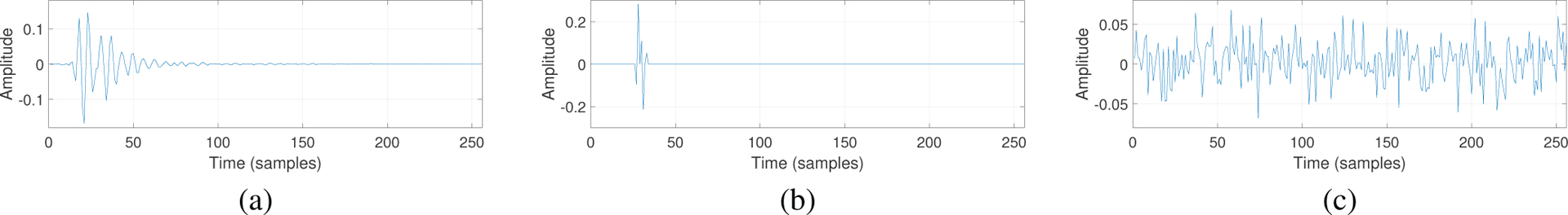
IRs of (a) quasi-sparse, (b) sparse, and (c) dispersive systems.

Fig. 2 presents the resulting MSE curves of using the SNLMS (24) as an example. The update rule (25) was used for ${\mathbf{\text{W}}}_n^2$, using c = 0.001. The normalization (26) was performed. The NLMS (3) is also compared. We used μ = 0.5 and δ = 0.01 for both SNLMS and NLMS. From the results we see that the selection of p is crucial for obtaining optimal performance for IRs with different sparsity degrees. For the quasi-sparse case in Fig. 2 (a), the fastest convergence is given by p = 1.5, which seems a reasonable value in terms of finding a balance between PNLMS (p → 1) and NLMS (p = 2). For the sparse case in Fig. 2 (b), p = 1.2 gives the best results, which is also intuitive since the sparsity level has increased. For the dispersive case in Fig. 2 (c), p = 1.8 results in the fastest convergence and is comparable to NLMS. These results show that the algorithm exploits the underlying system structure in the way we expect.

Fig. 2.

MSE of SNLMS with various p for (a) quasi-sparse, (b) sparse, and (c) dispersive systems.

Fig. 3 presents the mean of estimated filter coefficients to observe the converged solutions. The results were computed as the average of 500 iterations when the algorithm was in steady-state. In each case, we see that SNLMS (with the optimal p found in Fig. 2) converges to the same solution as NLMS, which agrees well with the corresponding true IR in Fig 1. This supports the argument that the proposed strategy of utilizing λ → 0⁺ provides the algorithms with the capability of leveraging sparsity without compromising estimation quality. In other words, the results together with Fig. 2 demonstrate that the sparsity promoting algorithms can exploit sparsity for speeding up convergence in the adaptation stage and perform equally well in steady-state should sparsity be present in the underlying system response.

Fig. 3.

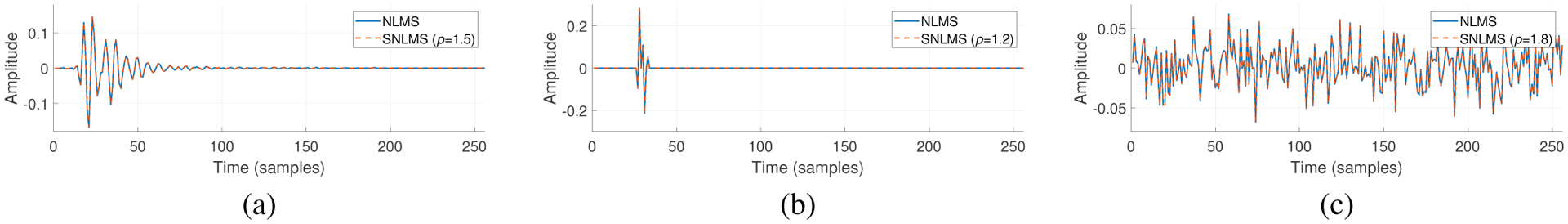
Mean of estimated filter coefficients for (a) quasi-sparse, (b) sparse, and (c) dispersive systems.

VI. Conclusion

In this paper, we exploited the connection between sparse system identification and SSR, and utilized the iterative reweighting strategies to derive novel proportionate adaptive filters that incorporate various diversity measures for promoting sparsity. Moreover, utilizing a regularization coefficient λ → 0⁺, the proposed SLMS and SNLMS algorithms can take advantage of, though do not strictly enforce, the sparsity of the underlying system if it already exists. Simulation results were presented to demonstrate the effectiveness of the algorithms.

References

- [1].Duttweiler DL, “Proportionate normalized least-mean-squares adaptation in echo cancelers,” IEEE Trans. Speech Audio Process, vol. 8, no. 5, pp. 508–518, 2000. [Google Scholar]
- [2].Benesty J, Gänsler T, Morgan DR, Sondhi MM, and Gay SL, Advances in Network and Acoustic Echo Cancellation, Springer, 2001. [Google Scholar]
- [3].Paleologu C, Benesty J, and Ciochină S, “Sparse adaptive filters for˘ echo cancellation,” Synth. Lect. Speech Audio Process, vol. 6, no. 1, pp. 1–124, 2010. [Google Scholar]
- [4].Lee C-H, Rao BD, and Garudadri H, “Sparsity promoting LMS for adaptive feedback cancellation,” in Proc. Eur. Signal Process. Conf. (EUSIPCO), 2017, pp. 226–230. [DOI] [PMC free article] [PubMed] [Google Scholar]
- [5].Lee C-H, Kates JM, Rao BD, and Garudadri H, “Speech quality and stable gain trade-offs in adaptive feedback cancellation for hearing aids,” J. Acoust. Soc. Am, vol. 142, no. 4, pp. EL388–EL394, 2017. [DOI] [PMC free article] [PubMed] [Google Scholar]
- [6].Widrow B and Stearns SD, Adaptive Signal Processing, Pearson, 1985. [Google Scholar]
- [7].Haykin S, Adaptive Filter Theory, 5th edition, Pearson, 2013. [Google Scholar]
- [8].Sayed AH, Adaptive Filters, John Wiley & Sons, 2011. [Google Scholar]
- [9].Manolakis DG, Ingle VK, and Kogon SM, Statistical and Adaptive Signal Processing: Spectral Estimation, Signal Modeling, Adaptive Filtering, and Array Processing, McGraw-Hill; Boston, 2000. [Google Scholar]
- [10].Wagner K and Doroslovački M, Proportionate-type Normalized Least Mean Square Algorithms, John Wiley & Sons, 2013. [Google Scholar]
- [11].Elad M, Sparse and Redundant Representations: From Theory to Applications in Signal and Image Processing, Springer, 2010. [Google Scholar]
- [12].Foucart S and Rauhut H, A Mathematical Introduction to Compressive Sensing, Springer, 2013. [Google Scholar]
- [13].Rao BD and Song B, “Adaptive filtering algorithms for promoting sparsity,” in Proc. IEEE Int. Conf. Acoust., Speech, Signal Process. (ICASSP), 2003, pp. 361–364. [Google Scholar]
- [14].Benesty J, Paleologu C, and Ciochină S, “Proportionate adaptive filters˘ from a basis pursuit perspective,” IEEE Signal Process. Lett, vol. 17, no. 12, pp. 985–988, 2010. [Google Scholar]
- [15].Martin RK, Sethares WA, Williamson RC, and Johnson CR, “Exploiting sparsity in adaptive filters,” IEEE Trans. Signal Process, vol. 50, no. 8, pp. 1883–1894, 2002. [Google Scholar]
- [16].Jin Y, Algorithm Development for Sparse Signal Recovery and Performance Limits Using Multiple-User Information Theory, Ph.D. dissertation, University of California, San Diego, 2011. [Google Scholar]
- [17].Liu J and Grant SL, “A generalized proportionate adaptive algorithm based on convex optimization,” in Proc. IEEE China Summit Int. Conf. Signal Inform. Process. (ChinaSIP), 2014, pp. 748–752. [Google Scholar]
- [18].Chen Y, Gu Y, and Hero AO, “Sparse LMS for system identification,” in Proc. IEEE Int. Conf. Acoust., Speech, Signal Process. (ICASSP), 2009, pp. 3125–3128. [Google Scholar]
- [19].Gu Y, Jin J, and Mei S, “l0 norm constraint LMS algorithm for sparse system identification,” IEEE Signal Process. Lett, vol. 16, no. 9, pp. 774–777, 2009. [Google Scholar]
- [20].Su G, Jin J, Gu Y, and Wang J, “Performance analysis of l0 norm constraint least mean square algorithm,” IEEE Trans. Signal Process, vol. 60, no. 5, pp. 2223–2235, 2012. [Google Scholar]
- [21].Wu FY and Tong F, “Gradient optimization p-norm-like constraint LMS algorithm for sparse system estimation,” Signal Process, vol. 93, no. 4, pp. 967–971, 2013. [Google Scholar]
- [22].Taheri O and Vorobyov SA, “Reweighted l1-norm penalized LMS for sparse channel estimation and its analysis,” Signal Process, vol. 104, pp. 70–79, 2014. [Google Scholar]
- [23].Wipf D and Nagarajan S, “Iterative reweighted ℓ1 and ℓ2 methods for finding sparse solutions,” IEEE J. Sel. Top. Signal Process, vol. 4, no. 2, pp. 317–329, 2010. [Google Scholar]
- [24].Gorodnitsky IF and Rao BD, “Sparse signal reconstruction from limited data using FOCUSS: A re-weighted minimum norm algorithm,” IEEE Trans. Signal Process, vol. 45, no. 3, pp. 600–616, 1997. [Google Scholar]
- [25].Chartrand R and Yin W, “Iteratively reweighted algorithms for compressive sensing,” in Proc. IEEE Int. Conf. Acoust., Speech, Signal Process. (ICASSP), 2008, pp. 3869–3872. [Google Scholar]
- [26].Candès EJ, Wakin MB, and Boyd SP, “Enhancing sparsity by` reweighted ℓ1 minimization,” J. Fourier Anal. Appl, vol. 14, no. 5, pp. 877–905, 2008. [Google Scholar]
- [27].Rao BD and Kreutz-Delgado K, “An affine scaling methodology for best basis selection,” IEEE Trans. Signal Process, vol. 47, no. 1, pp. 187–200, 1999. [Google Scholar]
- [28].Nash SG and Sofer A, Linear and Nonlinear Programming, McGraw-Hill Inc., 1996. [Google Scholar]