Host variables confound gut microbiota studies of human disease

Abstract

Low concordance between studies that examine the microbiota in human diseases is a pervasive challenge that limits capacity to identify causal relationships between host-associated microbes and pathology. Risks of obtaining false positives in human microbiota research are exacerbated by wide inter-individual heterogeneity in microbiota composition¹ likely due to population-wide differences in human lifestyle and physiological variables² that exert differential impacts on the microbiota. Herein, we infer the greatest, generalized sources of heterogeneity in human gut microbiota profiles and, further, identify human lifestyle and physiological characteristics that, if not evenly matched between cases and controls, confound microbiota analyses to produce spurious microbial associations with human diseases. Surprisingly, we identify alcohol consumption frequency and bowel movement quality as unexpectedly strong sources of gut microbiota variance that differ in distribution between healthy and diseased subjects and can confound study designs. We demonstrate that for numerous prevalent, high-burden human diseases, matching cases and controls for confounding variables reduces observed microbiota differences and incidence of spurious associations. Thus, we present a list of recommended host variables to capture in human microbiota studies for the purpose of matching comparison groups, which we anticipate will increase robustness and reproducibility in resolving true disease-associated gut microbiota members in human disease.

The gut microbiota plays a critical role in the development and function of several major organ systems, and dysregulation of this community can dramatically impact development of neurological, metabolic, and inflammatory diseases in murine models^3–5. Identifying gut microbiota members that causally contribute to human disease has proven difficult, and inter-individual microbiota variability may overpower true differences between diseased and healthy subjects in contemporary cross-sectional study designs. Via the American Gut Project (AGP), the largest known publicly available human gut bacterial microbiota dataset, we sought firstly to identify the most robust sources of human gut microbiota variability using machine learning strategies and subsequently to understand their impact on microbiota-centered study of human disease.

Machine learning framework

A table of 16S rRNA amplicon sequence variants (ASVs)⁶ was generated from stool samples of the AGP⁷ and was used to assess the strength of association between gut microbiota composition and each recorded questionnaire host variable. Association strengths were assessed using machine learning classification approaches that leverage bootstrapping and cross-validation to identify robust, replicable data patterns between groups. Binary case-control cohorts were constructed for each host variable, and the mean area-under-the-curve of the receiver operating characteristic (AUROC) was computed via Random Forests (Extended Data Figure 1). Resulting AUROC values quantify the ability of ASV abundance data to discriminate samples along a binary variable, and thus represent the robustness of associations between host variables and microbiota composition.

Microbiota-associated variable identification

We employed our machine learning framework firstly to determine strengths of microbiota associations with common exclusion criteria (Extended Data Figure 2A–B). Having considered for each putative exclusion variable its AUROC values, representation in the general human population, and relative samples sizes, we imposed new exclusion criteria (see Methods) to yield a final core population of 5,878 non-duplicate subjects. From this core population, balanced case-control cohorts were constructed to represent dichotomous responses for all questionnaire variables to assess their strength of association with gut microbiota composition using the aforementioned machine learning framework (Supplementary Table 1 for detailed case-control definitions). Numerous host physiological, lifestyle, and dietary variables exhibited significant microbiota associations (mean-AUROC>0.65 and P<0.05, Figure 1, Supplementary Table 2 for model performance data, Supplementary Table 3 for ASV importance data). Intriguingly, no human diseases reached AUROC>0.65 and P<0.05 (Extended Data Figure 2C) apart from those selected as exclusion criteria (i.e. inflammatory bowel disease and type 2 diabetes). Additionally, removing all subjects reporting any medical disease diagnoses yielded AUROC results concordant with those derived from the core sample population (Extended Data Figure 2D).

Figure 1: Physiological, lifestyle, and dietary characteristics strongly associate with gut microbiota composition.

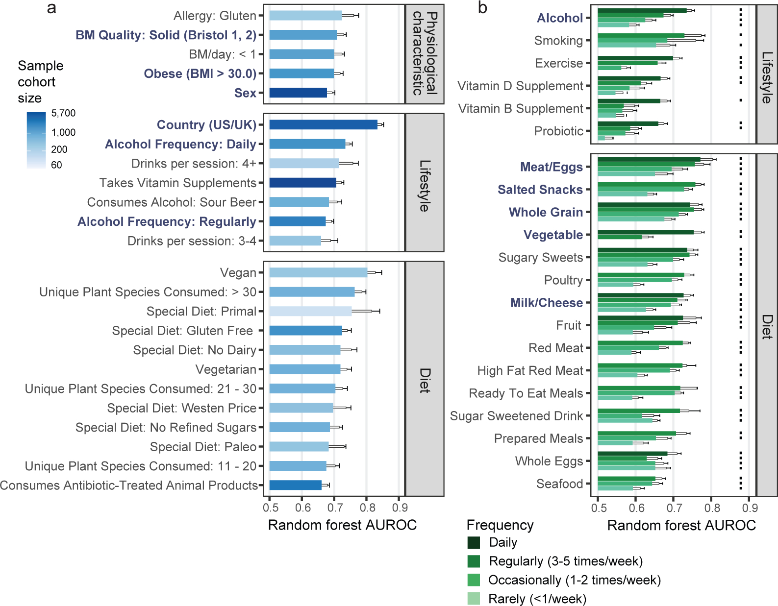
A) Random Forests analysis results for binary physiological, lifestyle, and diet variables. All variables shown exhibited P < 0.05 by empirical P value permutation tests. Blue labels are proposed as matching variables for examination in subsequent analyses (those of Figure 2 and beyond). B) Random Forests analysis results for frequency-based lifestyle and dietary intake variables. For each frequency category (i.e. ‘daily’, ‘regular’, ‘occasional’, and ‘rare’), binary cohorts were constructed with control subjects comprising those who self-reported ‘never’ for that variable. Frequency categories for each variable exhibiting P < 0.05 are denoted by dots over bars for frequency variables. In A and B, solid bars denote means, boxes denote upper inter-quartile ranges, and whiskers denote standard deviation of AUROC values from 100 repeats of Random Forests classifiers.

AUROC performances correlated with beta diversity analyses (Extended Data Figure 3A, Supplementary Table 2), though beta diversity metrics (i.e. R² effect sizes and F statistics) exhibited substantially stronger correlations with sample sizes than AUROCs and declared more microbiota-associated variables significant (Extended Data Figures 3A–D). Despite relative robustness to sample size, a threshold of n=500 cases and controls was found to maximize Random Forests model performance (Extended Data Figures 3E–F).

Host variables confound disease analyses

The gut bacterial microbiota has been established as a potent regulator of neurological, endocrine, and immune function in murine models. Interest in the role of this microbial community in human diseases that involve these systems has mounted, and a common strategy to understand whether gut bacteria may influence such diseases has been the cross-sectional survey study in which microbiota profiles of diseased subjects are compared to those of unaffected controls. If diseased subjects harbor unique distributions of physiological or lifestyle host variables that differ from those of controls, such cross-sectional studies may conflate disease associations with effects of confounding variables. Because we found that robust microbiota composition patterns were associated with several host variables, we sought to understand whether subjects reporting medically diagnosed diseases differed in their distribution of these host variables compared to randomly selected unaffected controls. Focus was placed on the following microbiota-associated variables based on their performance in machine learning analyses as well as redundancy with other host variables (Extended Data Figure 2E–H, discussed in Methods): BMI, sex, age, geographical location, alcohol consumption frequency, bowel movement quality, and dietary intake frequency of meat/eggs, dairy, vegetables, whole grain, and salted snacks. We found significant differences in the distributions of these microbiota-associated variables between cases and controls for most diseases (Figure 2A and Supplementary Table 4A–B). Microbiota comparisons of such cases and controls would thus identify differences linked to the disease as well as those driven by the microbiota-associated confounding variables. To remove the signal attributable to microbiota-confounding variables, we re-selected control subjects in a pairwise fashion by identifying for each case subject a control individual that was matched for values of each microbiota-confounding variable using a Euclidean distance-based process (detailed in Methods). Community composition differences between cases and controls were assessed for disease cohorts matched for microbiota-confounding host variables and cohorts that were unmatched save for location using standard beta diversity-based PERMANOVA tests, an ecology-based community-level approach commonly used to test microbiota differences in disease^8–10. As compared to location-only pairing, a reduction in microbiota community differences was observed for 13/19 diseases when matching for the presently identified microbiota-associated confounding variables (Figure 2B), despite no changes in sample sizes. These findings were consistent when excluding all subjects reporting medical diagnoses of any disease from the control populations (Extended Data Figure 4), and when using machine learning-based approaches (Extended Data Figure 5A). Statistically significant microbiota differences were lost when cases were compared to confounder-matched controls for several diseases including clinical depression, autism spectrum disorder (ASD), lung disease, thyroid disease, migraine, and small intestinal bowel overgrowth (SIBO).

Figure 2: Human disease subjects vary from healthy controls in critical microbiota-associated variables that confound microbiota analyses.

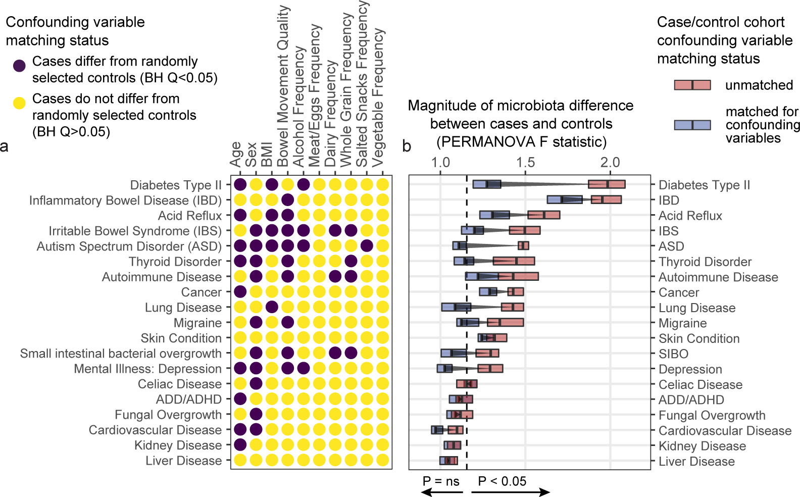
A) Shown in purple are variables that differ in disease cases versus randomly selected location-paired control subjects (Benjamini-Hochberg Q value < 0.05). For continuous variable comparisons (age, BMI) a two-sided Mann-Whitney U test was performed, while for remaining categorical variable comparisons a Fisher’s exact test was performed. B) Shown are differences between beta diversity-based F statistics of unmatched, location-paired disease case-control cohorts and those of fully matched case-control cohorts. Analyses were augmented using a bootstrapping control cohort re-selection method to assess dispersion of microbiota community differences (described in Methods). Red boxes represent interquartile ranges in F statistics from 25 randomly selected location-paired unmatched cohorts, while blue boxes represent interquartile ranges in F statistic from 25 randomly selected cohorts for which controls were selected that matched cases for all microbiota-associated host variables that differed between cases and controls shown in (A). Center lines within boxes represent median F statistic values.

The greatest drop in microbiota differences between cases and controls after matching for confounding variables occurred for subjects reporting medical diagnoses of type 2 diabetes (T2D). Prior to matching, T2D subjects differed markedly from controls in terms of alcohol intake frequency, BMI, and age (Figure 3A–C). Gut microbiota profiles differed significantly between T2D cases and controls both by machine learning analyses and by beta diversity-based permutation tests (Figure 3D). Upon matching T2D cases and controls for microbiota-associated confounding variables (Figures 3E–G), a significant microbiota difference between cases and controls was not observed by machine learning analyses, while a substantially reduced (though still statistically significant) difference was observed by beta diversity-based tests (Figure 3H–I). This reduction in apparent diabetes-associated microbiota signal was reflected in taxon-level analyses on matched versus unmatched cohorts (Extended Data Figure 5B).

Figure 3: Microbiota variation due to confounding variables spuriously increases observations of disease-associated microbiota differences.

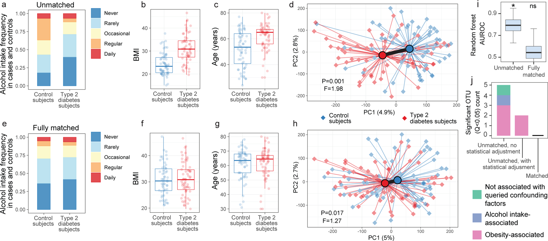
(A-C) Differences between type 2 diabetes subjects and non-diabetic control subjects (N=126) for alcohol frequency (Benjamini-Hochberg [BH] Q=0.0015, Fisher’s exact test) (A), BMI (BH Q=4.14*10⁻⁹, two-sided Mann-Whitney U test) (B), and age (BH Q=5.94*10⁻⁵, two-sided Mann-Whitney U test) (C). D) Principal coordinates analysis (PCoA) plot of diabetes cases and control subjects unmatched for aforementioned variables, with median PERMANOVA P value and F statistics shown. Subject group centroids are depicted by an outlined circle. (E-G) Differences between type 2 diabetes subjects and fully matched non-diabetic control subjects for alcohol frequency (E), BMI (F), and age (G). H) PCoA plot of confounder-matched diabetes cases and controls. I) Random Forest AUROC values for diabetes cases and controls before and after matching for confounding variables. J) Linear mixed effects models were constructed as described in Methods to include age, BMI, and alcohol intake frequency as confounding covariates. Shown are ASVs that passed BH Q values < 0.05 cutoffs for each analysis. Boxes denote inter-quartile range, black bar denotes median, and whiskers denote range.

Strategies to collapse the effect of confounding variables include statistical adjustments in linear mixed model frameworks. We found that adding BMI, age, and alcohol intake as covariates in linear mixed effects models reduced numbers of spurious ASVs identified as significantly differing between unmatched T2D cases and controls from 5 to 2 (Benjamini-Hochberg Q<0.05). However, the only ASVs differing significantly between T2D and controls after statistical adjustment for confounding covariates were spurious observations - defined as those that differ in subjects based on confounding variables independent of disease (Figure 3J, Supplementary Table 5), suggesting that statistical adjustments can fail to discern true signal from confounding factors. In contrast, no ASVs differed significantly when matching subjects by confounding variables (Figure 3J), highlighting the importance of subject selection in mitigating false positive associations. These observations were mirrored with more relaxed significance cutoffs for ASVs differing between diabetics and non-diabetic controls (P values<0.05) as well as when confounder-associated ASVs were identified using ANCOM¹¹ (Extended Data Figure 6).

Examining prior studies that sought to identify taxa associated with T2D^{8–10,12–14}, we find that only one of six reported alcohol frequency for cases and controls. One out of six T2D studies were matched for two of the three variables of BMI, age, and alcohol frequency, three of six studies were matched for just one of the three confounding variables, and the remainder were either fully unmatched or did not report data for these variables (Extended Data Figure 7A). Analysis of three such studies investigating T2D^8,9,14 and one examining metabolic syndrome¹⁵ revealed that matching by one or more confounding variables significantly decreased observed microbiota differences between cases and controls, a finding replicated in all four studies (Extended Data Figure 7B–C). The effect of the antidiabetic drug metformin on the gut microbiota was also diminished when comparing to confounder-matched subjects (Extended Data Figure 7B). Though we report a retention of significant differences between cases and controls even after matching, an independent study reported no significant differences in gut microbiota profiles between obese diabetics and obese controls¹⁰, highlighting the potential importance of matching for confounding variables in T2D.

Notably, several diseases were associated with differences in gut microbiota community composition even after matching for the confounding variables investigated herein. These diseases included inflammatory bowel disease (IBD), subjects reporting any skin condition, acid reflux, and cancer. Shifts in individual ASV abundances in IBD subjects shared several features with prior studies^16–18, showing reductions in Ruminococcaceae, Rikenellaceae and Lachnospiraceae members (Supplementary Table 6).

Alcohol & stool quality impact microbiota

Surprisingly, alcohol consumption robustly segregated microbiota profiles and did so in a dose-dependent manner (Figure 1B). We sought to quantify the extent to which alcohol intake frequency may confound microbiota-disease associations. Toward this end, we employed two independent approaches: leave-one-out (LOO) matching for all variables but one, and matching by a single variable in isolation. We found that alcohol consumption exhibited non-zero confounding effects in several diseases by both methods and was not limited to T2D (Extended Data Figure 8A–B). For T2D, matching for all variables except alcohol (LOO) exhibited an increase in apparent microbiota differences between cases and controls as compared to matching for all variables, indicating a significant, non-redundant confounding effect for alcohol in this population (Figure 4A). Similarly, matching for alcohol intake frequency alone significantly collapsed microbiota differences between T2D cases and controls (Figure 4A), emphasizing the confounding capacity of this host variable in microbiota comparisons.

Figure 4: Alcohol intake and bowel movement quality are associated with robust effects on microbiota composition that confound microbiota studies of human disease.

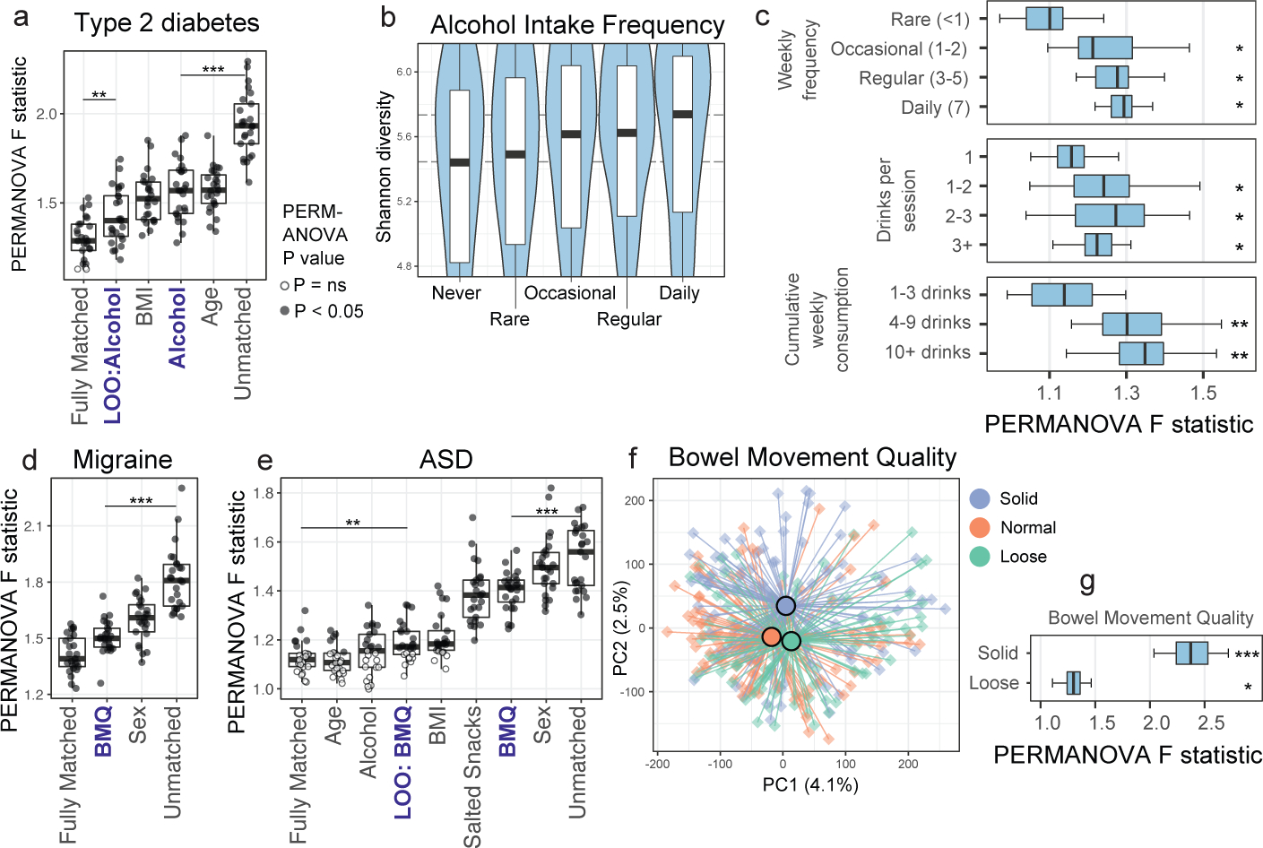
A) Case/control cohorts for type 2 diabetes were constructed by matching for no host variables (‘Unmatched’), matching for all three discordant variables together (‘Fully Matched’), and matching for either each variable individually or all variables but one in a leave-one-out (LOO) analysis (with the left-out variable indicated after ‘LOO’). Microbiota association estimates were quantified using beta diversity-based F statistics as described in the text. Significance of differences in F statistics was assessed by two-sided Student’s t-test. P=0.002, P=2.7*10⁻¹¹. B) Shannon diversity by alcohol frequency categories. Thick black bars represent median values, boxes delineate quartile values. Spearman P=4.8*10⁻¹⁴. C) Alcohol subjects were matched to non-drinker controls for confounding variables (Extended Data Figure 9C) and bootstrapped beta diversity F statistics were calculated. Median PERMANOVA P values are shown. P=0.021, P=0.011, P=0.006; P=0.018, P=0.01, P=0.016; P=0.004, P=0.004. D) Cohorts were constructed as in (A) by matching by one variable individually or LOO analyses as indicated. P=1*10⁻¹⁰. E) Single-variable matching and LOO cohorts were similarly constructed for ASD. P= 0.004, P=8*10⁻⁵. F) Canberra-based PCoA ordinations depicting solid, normal, and loose bowel movement quality (BMQ) subjects (Bristol stool scores 1–2, 3–4, and 5–7, respectively). Group centroids are depicted by large dark-outlined circles. Inter-group PERMANOVA P = 1*10⁻⁵. G) BMQ subjects were matched to controls for confounding variables (Extended Data Figure 10A) and bootstrapped beta diversity F statistics were calculated. Boxes denote inter-quartile range, black bar denotes median, and whiskers denote range. Median PERMANOVA P values are shown. P=0.0003, P=0.006. * P < 0.05; ** P < 0.005; *** P < 0.0005.

To validate effects of alcohol consumption on the gut microbiota, we examined an external cohort¹⁹ for which 16S rRNA and alcohol consumption data were recorded. Genus-level differences between frequent alcohol consumers and infrequent consumers were consistent between the present study and the external cohort (Spearman P=5*10⁻⁵, ρ=0.54, Extended Data Figure 9A). Among taxa that differentially abundant between non-drinkers and all alcohol consumer cohorts, a Bifidobacterium ASV was most frequently enriched among alcohol consumers (Extended Data Figure 9B), a finding supported by prior studies in smaller cohorts^20–22. Alpha diversity also increased in a dose-dependent manner among alcohol consumers (Figure 4B), mirroring prior findings examining red wine consumption²³.

Alcohol consumption frequency itself was robustly associated with differences in the distribution of several microbiota-confounding variables as compared to non-drinkers (Extended Data Figure 9C). Upon selecting matched controls, a detectable dose-dependent effect on the microbiota remained observable for all categories of alcohol consumption, while cumulative drinks per week exhibited the most robust microbiota differences by ecological (Figure 4C) and machine learning approaches (Extended Data Figure 9D). When examining types of alcohol consumed, wine and beer/cider consumption were associated with the greatest differences in microbiota composition (Extended Data Figure 9E) and alpha diversity (Extended Data Figure 9F).

Bowel movement quality (BMQ) was among the top confounding variables across diseases using both methods of confounding effect estimation (Extended Data Figure 8A–B). In the case of migraine and ASD, omitting BMQ from matching variables caused the greatest increase in case-control microbiota differences, indicating its non-redundant impact on microbiota variance, a finding replicated when matching for BMQ alone (Figure 4D–E). Similarly to alcohol consumption, subjects reporting abnormal BMQ exhibited differences in their distribution of confounding variables compared to controls (Extended Data Figure 10A). Upon selecting confounder-matched subjects, the strength of association of BMQ with microbiota composition remained evident by ordination (Figure 4F) and PERMANOVA (Figure 4G). Genus-level abundance shifts were concordant between our dataset and an independent study¹⁵ performed on a separate continent (Extended Data Figure 10B).

Caveats to data interpretation

Small sample sizes can produce false negatives, and beta diversity-based analyses were indeed strongly associated with sample size (Extended Data Figure 3). Random Forests AUROC values were less dependent on sample size, but a performance plateau was observed at n=400–500 subjects for most variables (Extended Data Figure 3E–F), a threshold that many disease cohorts did not reach in our dataset. Depression may be one such example (n=342), and a recent larger study matched for key variables reported depression-associated microbiota differences²⁴.

Self-reporting of personal information can lead to bias and misreporting which can corrupt datasets. Caveats including the observer effect exist in professional-assisted reporting as well, thus novel objective measurement techniques (e.g. DNA metabarcoding²⁵) or combinations of approaches may better estimate real effects. Regardless, well-reported associations between disease states and host variables were recapitulated in our dataset (e.g. thyroid disease in females, cardiovascular disease in males, higher BMI in T2D, among others), strengthening confidence in the self-reporting within this dataset. However, it is possible that matching diabetic subjects for confounding variables enriched for undiagnosed diabetics being chosen as controls, highlighting the need for further study involving clinically verified control subjects. Matching-variables examined in the present study were pared to eliminate redundant, co-correlated host variables; however, high-AUROC variables that were omitted may have unique distributions in other populations. Thus, examination of all high-performing variables may uncover confounding biases. Additionally, the administered questionnaire may not have captured all extant confounding variables. Investigation of additional putative microbiota-confounding factors such as sexual practice²⁶, immigration status, socioeconomic status, medication use, etc., are likely to further increase resolution on true disease-associated microbiota members.

The present study queried the 16S rRNA gene V4 region, which has variable efficacy in resolving clades with resolution typically at the genus level, and strain-level differences in diseased subjects may exist for those reported herein as not differing significantly from control subjects. A prior report found that specific gut taxa including Enterobacteriaceae members bloom during sample transport, prompting their removal from our analyses²⁷. Such bacteria have been associated with human inflammatory disease^16,28, and thus estimates of microbiota differences for diseases in which these taxa are differentially abundant would have been underestimated. Additionally, while we found that statistical correction for confounding variables did not eliminate the appearance of spurious confounder-associated taxa within comparative analyses, it is unclear what degree of mismatching is statistically tolerable among different disease comparisons. In lieu of a demonstration of tolerance of analyses to confounding variable mismatch, we propose matching cases and controls to minimize risks of type I errors.

The AGP subjects examined were not representative of the global human population with regards to racial and ethnic demographic composition, and though we found concordant effects of bowel movement quality on an external cohort comprising an ethnicity not captured robustly in the AGP, effects and identities of confounding variables across ethnic populations may differ in scale and quality. Furthermore, ethnicity itself may exert a confounding effect²⁹ that our dataset was unable to address due to insufficient ethnic diversity. Our dataset was representative, however, with regards to burden of chronic disease, and to maximize generalizability of our findings we permitted inclusion of subjects within each disease comparison that reported other diseases. While it is possible that other diseases contributed confounding effects in each disease analysis, it is noteworthy that diseases apart from those included in exclusion criteria (T2D, IBD) had minor impacts on the microbiota compared to other variables (Extended Data Figure 2C) and did not meet or approach our standards for selection of exclusion/matching variables. However, removing subjects reporting any disease from the control population increased differences between cases and controls (Extended Data Figure 4C–D), suggesting that despite confounder matching, other microbiota-associated host variables not robustly captured in our study (such as socioeconomic status, ethnicity, medication usage, etc.) may differentiate disease-free subjects from those with chronic diseases. Thus, choices of comparison groups can significantly impact resulting observations and should be considered carefully during the course of study design. Stool does not represent well microbial populations of the upper gastrointestinal tract³⁰, which may explain the lack of signal observed for SIBO after matching. Finally, while matching for confounding variables narrowed the list of disease-associated individual taxa for most diseases, it remains possible that confounder-associated microbial taxa that do not differ in abundance between matched cases and controls still modulate pathogenesis in subjects with genetic predispositions to disease³¹ (or other environmental predispositions). Thus, an aberrant host interaction with microbiota members prevalent in healthy subjects may constitute a mechanism of pathogenesis that cannot be addressed by association studies at present.

Discussion

We believe our results underscore the need to match human cases and controls by the identified microbiota-confounding host variables, especially in studies examining diseases/phenotypes linked with unique physiology, lifestyle, or dietary traits. Our results are in accord with prior studies that found associations between the gut microbiota and stool quality, BMI, age^2,32, as well as red wine consumption²³ and salt intake³³. Evidence suggests whole grain does not affect gut microbiota composition differently than refined grain³⁴, and thus the effect of whole grain in our study may have been driven primarily by general grain consumption. Our work finds find that matching disease subjects to controls by confounding variables representing the largest sources of microbiota heterogeneity reduces disease associations with spurious bacterial taxa and increases likelihood of identifying taxa truly associated with disease. We posit that rigorous matching will increase concordance between microbiota studies in human disease and will accelerate understanding of the role of gut microbes in pathogenesis. The present work also emphasizes the value of large human cohorts with well-collected metadata. Establishment of such large cohorts, preferably in a longitudinal framework so as to reduce effects of inter-individual confounding variables, with the inclusion of other sample types amenable to omics analyses beyond the gut microbiota, have a high likelihood of contributing substantially to our understanding of health and disease.

Methods

American Gut cohort characteristics, study design, and data availability

The American Gut Project was designed and managed by the American Gut Consortium⁷. Participant volunteers paid a nominal fee and received a collection vessel and a questionnaire. Samples were self-collected and shipped at room temperature to central locations for DNA extraction and sequencing of the V4 hypervariable region of the 16 rRNA gene, as described in the first original AGP publication⁷. The sequencing data used herein are available at the European Bioinformatics Institute (EBI) database under study accession ID: MGYS00000596, and this database is continually updated to add most recent participants in the project. Participant consent was obtained under Institutional Review Board human research subject protocols from the University of Colorado, Boulder (protocol #12–0582; December 2012 to March 2015) or from the University of California, San Diego (protocol #141853; February 2015 to present). No personally identifiable data are included in the public database nor were accessed in the present study.

Processing of sequencing data

Raw fastq files were downloaded from EBI and processed using the ‘dada2’ R package⁶. Reads were truncated at length of 150 bp, a maximum expected error threshold of 1 was imposed, and reads were truncated at the first base with Q score of 11 or below. Taxa shown to be prone to blooming in the process of transporting American Gut Project fecal samples⁷ were removed from analysis. Taxonomy was assigned using the Silva 128 ribosomal RNA database using the RDP Naive Bayesian Classifier algorithm default in dada2 (v1.14.1). Sequence variants that were present in fewer than 50 samples (0.27% of total samples) and in lower total relative abundance than 0.01% were removed from analysis, and samples were rarefied to 10,000 reads while removing samples with reads fewer than 10,000. Sequence variants were assigned names equivalent to md5sums of their fasta 16S sequences (R package ‘digest’).

In total, 19,990 fastq files were downloaded from EBI, of which 12,339 gut microbiota samples remained after rarefying to 10,000 reads per sample. Some participants chose to sequence their microbiota more than one time over the course of varying time periods, which after limiting each participant to one gut sample, narrowed sample numbers to 10,366. Samples that did not input answers in their questionnaire relating to confounding variables of interest (BMI, age, sex, alcohol intake frequency, bowel movement quality, vegetable, meat/eggs, dairy, and salted snacks intake frequency) were removed from consideration. Finally, only samples of participants currently residing in the US, UK, and Canada were used, leaving 5,878 that were defined as belonging to the core selection population after imposition of exclusion criteria selected as explained below.

Construction of simulated paired-sample studies for machine learning analyses

From the questionnaire, participants were asked a range of questions related to age, sex, health, lifestyle, disease status, and diet frequency. From these questions, a majority were able to be defined as a binary variable with a positive and negative class (e.g. type 2 diabetes status), which allowed for simple construction of a subset of the samples to be used for binary classification of the questionnaire variable. Given a binary questionnaire variable, the cohort was constructed from a subset of the selection population that answered the question. Given the selection population that reported true or false to a cohort variable, pairwise Euclidean distances were computed between the positive and negative groups from the given set of matching variables that were normalized to zero-mean and unit-variance (centered and scaled). Iteratively, a positive sample and the closest negative sample by Euclidean distance were removed from the selection population and added to the cohort, which was continued until no positive samples remained in the selection population. At the end of the procedure, the constructed cohort had a balanced number of cases and controls. For all cohorts examined for exclusion/inclusion criteria selection (Extended Data Figure 2), for those examining effects of questionnaire variables in the core population (Figure 1), and for unmatched disease cohorts (Figures 2–3), each control subject was paired with a case subject closest in geographical proximity in order to emulate current cross-sectional studies for which samples are commonly collected from a single research center. Specifically, sample latitude and longitude values were used to calculate the Euclidean distances described above. Where country information was available for samples but city was unavailable, coordinates for the centroid of the country were used. Cohorts were constructed for all questionnaire variables that had an adequate number of samples (n ≥ 50), selecting from samples that had reported specific metadata variables (age, BMI, sex, location, antibiotics, as well as IBD, type 2 diabetes for inclusion/exclusion criteria selection as performed in Extended Data Figure 2). All cohorts were capped at 1,500 subjects (750 cases and controls) for machine learning analyses, and the top 750 closest pairs (with smallest Euclidean distance) were chosen. For a subset of variables, case-control cohorts were specially constructed using customized selection criteria (e.g. intra-uterine device control subjects were selected from the female population only, individuals with BMI>40 were included in control subjects for type 2 diabetics to correspond to the range of BMI in type 2 diabetics). A full list of questionnaire variable cohorts is listed in Supplemental Table 1.

Diet frequency variables were present in the questionnaire for a set of standard foods and beverage types, for which participants recorded their consumption frequency from a set of 5 values: Daily, Regularly (3–5 times per week), Occasionally (1–2 time per week), Rarely (less than once a week), and Never. Binary matched cohorts were constructed from diet frequency variables where healthy participants that belonged to ‘daily’, ‘regularly’, ‘occasionally’, and ‘rare’ consumption groups were matched with the set of participants that belonged to the ‘never’ group, which was taken as the negative class. In cases of under-sized ‘never’ or ‘daily’ frequency groups (where n < 200), subjects responding ‘never’ were combined with adjacent frequency groups successively until n > 200 to increase power for modeling, and the same was done for under-sized ‘daily’ cohorts in that they were combined with adjacent frequency groups until n > 200. This threshold was relaxed to 100 when considering only subjects not reporting diseases (analyses of Extended Data Figure 2C–D) to account for loss of power (N=2,971 disease-exclusive population vs. N=5,878 disease-inclusive population).

Machine learning classification of host-related variables

Support vector machines (SVM) analysis was used to determine whether microbiota profiles were predictive of age as a multi-class variable (Extended Data Figure 2B), with age groups binned at 5-year intervals for achieving sufficient power per group. All subjects aged 75 and older were binned into a single group. SVM models were trained over 10-repeat 10-fold stratified cross-validation. Age groups that were overrepresented compared to others were down-sampled to 350 subjects to avoid overfitting to those groups. Additionally, each age group maintained a standard ratio of participants belonging to the US and the UK to mitigate the classifier learning geographic location-associated microbiota patterns that could be erroneously attributed to age groups. For this multi-class variable, Random Forests were also run but yielded prediction accuracy results lower than those using SVM.

For binary cohort machine learning analyses, Random Forests classifiers were used to infer the ability of host microbiota data to discriminate between response groups. Machine learning models were first trained on a subset of the dataset (i.e. the training set), and then were applied to the remaining data (i.e. validation set), in order to infer the ability of the model to classify new, unseen data. Random Forests was set to have 512 decision trees, with a bootstrap sample size set to 70% of the training set, and the maximum set of features considered when splitting a node was set to the square-root of the total number of features. Maximum depth was set to allow the trees to grow until each leaf contained one sample. These choices were made to force maximum variance between base-learner decision trees, which when aggregated, help eliminate the concern for overfitting on the training-set. This was a strong need as some cohorts had few samples relative to the number of OTU features used for classification. A 25-repeat stratified 4-fold cross-validation was used to obtain a distribution of random forests prediction evaluations on a validation set. In 4-fold cross validation, the cohort is split in a stratified fashion into 4 subsets of equal size, where each subset is held out as the validation set, with the remaining subsets being used as a training set. (ie. 75% training set, 25% validation). Pairs were not enforced to be included in the same set, training or validation, so stratification was implemented in order to maintain class balance in each set. The above framework allows for an estimate of the generalizability of the classifier to model the discriminatory features of the microbiota between positive and negative classes. To address the concern that the classifiers were overfitting noise in ASV abundance data, for each iteration of the cross-validation, the response variable for each sample was randomly permuted (‘shuffled’) and a classifier was trained on the corrupted dataset. The results of the randomized classification results were taken as a null distribution in order to compute an empirical P value that represents the significance of the cross-validation models’ ability to discriminate between true classes compared to randomized classes.

The accuracy and discriminatory power of the models were assessed using the area-under-the-curve of the receiver-operating characteristic curve (AUROC). The receiver-operating characteristic curve represents the relationship of the true positive rate versus the false positive rate of the classification of the validation set as the binary probability prediction threshold is swept from 1 to 0. The area-under-the-curve can be interpreted as the probability, given a random pair of positive and negative samples, that the classifier will predict the positive class probability of the positive sample higher than the negative sample. AUROC values range from 0.5, denoting prediction equivalent to random choice, to 1.0, a perfect classifier. The mean-AUROC value across 100-iteration distribution of cross validation models was used as an estimated association between host variable and microbiota signals. An empirical P value was used, defined as the percentage of classifiers with lower AUROC values than the mean-’shuffled’-AUROC value over all 100 iterations of the cross-validation procedure³⁵. Specifically, the empirical P value was defined as:

$$p=\frac{\left|\left\{D\text{'}\in \widehat{D}:e\left(f,D\text{'}\right)\le e\left(f,D\right)\right\}\right|+1}{k+1}$$

where D’ is the ‘shuffled’ permuted dataset, and e(f, D) is the error of the function f learned on dataset D. The empirical P value thus is taken to represent the fraction of classifiers that performed worse than the averaged shuffled classifier performance. SVM, Lasso and XGBoost were also performed on all ‘Phase I’ exclusion variable analyses to compare to Random Forests. SVM, Lasso, and XGBoost all underperformed as compared to Random Forests in terms of AUROC values for these variables. All machine learning analyses were performed in Python 3.6.10 using seaborn, numpy, pandas, matplotlib, scikit-learn, xgboost, and scipy. R packages used for visualization of all analyses include: reshape2, superheat³⁶, ggplot2, RColorBrewer, ape, viridis, labdsv, stringr, plyr, dplyr, grid, digest, forecast, ade4, gridExtra, biomformat, and lattice.

Establishing core sample dataset via inclusion/exclusion criteria selection

Heterogeneity in human populations is a well-appreciated phenomenon that weakens statistical analyses by reducing resolution on the variable of interest (e.g. disease state). Efforts to deconvolute this heterogeneity include the imposition of exclusion criteria to eliminate subjects that are outliers among the measurements of interest (e.g. subjects exhibiting great differences in microbiota composition) so as to restrict study to a more homogeneous (and thus less confounded) core population within which to make comparisons. Common exclusion criteria for microbiota studies were examined including temporal proximity to last antibiotic usage, BMI, age, type 2 diabetes, and inflammatory bowel disease (IBD)⁷. To independently test the microbiota impact of these common exclusion/inclusion criteria is order to evaluate and select criteria for our own study, we applied Random Forests and SVM analyses on an initial cohort of subjects (N = 4,038). These subjects were themselves chosen according to previously used exclusion/inclusion criteria, specifically: no medical diagnoses of IBD or type 2 diabetes, BMI within 18.5 and 30, age within 20 and 69 years, no antibiotics usage within 1 year of fecal sampling, and subjects from the top three countries sampled in the AGP (USA, United Kingdom, and Canada). The last inclusion criterion was imposed due to prior indications of microbiota effects by geographical origin¹⁵. For clarity and to distinguish these analyses from subsequent analyses, we term this investigation of common inclusion/exclusion criteria as ‘Phase I’ in Supplementary Table 1A, where cohort sizes, negative and positive class definitions, as well as inclusion/exclusion criteria for this analysis itself can be found. These criteria were applied to all subjects for consideration except for cases in which that variable was being assessed (e.g. for assessing microbiota effects of IBD, cases included IBD subjects). To select exclusion/inclusion criteria for subsequent analyses, we next considered for each putative exclusion variable its capacity to be predicted by the microbiota in this first phase of analysis, its representation in the general human population, its relative sample size in our dataset, and prior literature as follows. Balanced location-matched cohorts were constructed for each variable, and the aforementioned Random Forests framework was performed. AUROC data from this phase of analysis are shown in Extended Data Figure 2A. Via this analysis, variables with AUROC values > 0.7 were prioritized as having strong microbiota associations. All subjects within positive classes of variables within this high microbiota association group of variables represented small proportions of the study population and thus were good candidates for exclusion, encompassing outlier microbiota compositions. An exception was country of residence, for it represented a variable with high numbers of samples with differing responses (specifically, USA, UK, and Canada) that should thus not be considered indicative of an outlier microbiota composition profile. This variable was not chosen for exclusion due to the intention to match cases and controls for location in all analyses as part of simulating real-world studies performed at a single research center, in which cases and controls are inherently matched for location. Age < 20 years was chosen as an exclusion criterion, as age 20 was a demarcation point for age-based microbiota predictability as seen in SVM classification accuracy (Extended Data Figure 2B), after which age predictability of age based on microbiota profiles exhibited a decline. Some commonly excluded groups yielded low model performance, such as underweight subjects, seniors ages 70+, and subjects reporting antibiotic use within 6 months to a year, and were thus not chosen as exclusion criteria. These groups were either not significant by permutation tests (P < 0.05) or had very low classification accuracy (AUROC < 0.6), and comprised large numbers of samples. The upper-limit of BMI values allowed was also extended to 40 despite their relatively high discriminatory power (AUROC = 0.69) so as to include a larger number of participants and to maximize generalizability of our findings to general populations which exhibit increasing obesity incidence in both the developed and developing worlds³⁷. While microbiota profiles of subjects who reported antibiotics usage within 2–6 months of sampling performed with similar discriminatory power to that of the obese subject cohort, it remained excluded due to uncertainty in the recency of the given antibiotic use event, with prior literature demonstrating a near-complete restoration of community composition within that time range³⁸, as well as uncertainty over the types of antibiotics used by participants.

Thus, exclusion criteria that were imposed for the analysis of Figure 1 (termed ‘Phase II’ analysis in Supplementary Table 1B) and all subsequent analyses were as follows: no medical diagnoses of IBD or type 2 diabetes, BMI within 12.5 and 40, age within 20 and 80 years, no antibiotics usage within 6 months of fecal sampling, and subjects from the top three countries sampled in the AGP (USA, UK, and Canada). This yielded a final core sample population of N = 5,878 subjects. Special cohorts were constructed for all variables in which cases were defined as one of the exclusion variables (e.g. IBD), or as denoted in Supplementary Table 1B for the specific variables of autism spectrum disease, hormonal intra-uterine device use, and contraceptive pill use.

Selection of host variables for matching

We constructed balanced location-matched cohorts with exclusion/inclusion criteria described above, and performed our Random Forests pipeline on the resulting core sample population (referred to as ‘Phase II’, results shown in Figure 1 and Supplementary Table 2, with cohort sizes, population size, and class definitions in Supplementary Table 1B). Having found numerous host variables with strong effects linked to the microbiota (AUROC > 0.7) via this analysis, we sought to pare down the list of those to consider for examining potential confounding effects in human disease (i.e. to identify ‘matching’ variables for human disease analyses of Figure 2). Firstly, we sought to omit redundant variables that were highly co-correlated with others, so as to prevent over-matching and to reduce the burden of data collection in hypothetical future studies. To identify such inter-variable relationships, a Spearman test co-correlation map was generated by converting the ordinal frequency of consumption variables to numeric values and running pairwise Spearman correlations on all variables for which at least one frequency category (e.g. daily, occasional) exhibited AUROC > 0.7 and P < 0.05 by Random Forests (Extended Data Figure 2C). Variable redundancy was defined by a Spearman (R package ‘Hmisc’) rho value > 0.3 between two variables. The highest AUROC variable amongst a pair or group of such co-correlated variables was then selected as a matching variable (e.g. poultry and red meat intake frequency both correlated strongly with meat/eggs frequency [rho > 0.3], while meat/eggs had a higher AUROC). Thus, one variable from within each major branch of the metadata variable co-correlation tree in Extended Data Figure 2E was chosen as a representative of the variables inhabiting the same branch. The binary variables of a no gluten diet, gluten allergy subjects, and subjects taking vitamin supplements could not be assessed via Spearman correlation, and thus Mann-Whitney U tests (R package ‘exactRankTests’) were performed (all two-group statistical tests in the study were two-sided) to test differences in all frequency diet variables between the cases and gluten-eating controls. We found that whole grain consumption frequency differed significantly between no gluten diet subjects and controls as well as gluten allergy subjects and controls (Extended Data Figures 2F–G), indicating a degree of redundancy and thus we opted to retain whole grain consumption in place of the two binary variables for matching. Similarly, age was strongly correlated with the binary variable of vitamin supplement intake (Extended Data Figures 2H), indicating redundancy. Finally, age was associated with smoking frequency via a non-monotonic relationship (Extended Data Figure 2I), which was tested and confirmed by the Hoeffding’s D test (R package ‘DescTools’). Having identified non-redundant variables with AUROC > 0.7, we next considered variables with lower microbiota association strengths (0.65 < AUROC < 0.7) that had either extensive precedent for matching, known associations with human disease, or great variation among human populations, for which sex met all four criteria. The final chosen matching variables are subsequently referred to in the main text as microbiota-confounding variables and were thus comprised of: BMI, sex, age, geographical location, alcohol consumption frequency, bowel movement quality, and dietary intake frequency of meat/eggs, dairy, vegetables, whole grain, and salted snacks.

This Phase II analysis was also performed on a sample population with the additional exclusion criterion to remove all subjects reporting medical diagnoses of any disease (Extended Data Figure 2C–D, total population size = 2,971), and cohorts within this analysis were termed “disease-exclusive” cohorts. For these analyses, each disease cohort consisted of cases that reported no diseases except for the disease being examined. Results were concordant among this analysis and the prior analysis with only IBD and type 2 diabetes excluded (“disease-inclusive” cohorts), as per exclusion criteria stated above (Extended Data Figure 2D). Importantly, all proposed matching variables were the top-performing variables in both analyses.

Examination of confounding variables in human disease subjects

To identify microbiota-associated host variables that differed significantly in their distribution between disease cases and controls (and thus confounded analyses), balanced case control cohorts were constructed for each disease captured in the AGP dataset. Each cohort was assembled by selecting one location-paired control for each case from the core sample population. Specifically, latitude and longitude numeric values were used to construct Euclidean distance matrices encompassing all cases (respondents having selected “Diagnosed by a medical professional [doctor, physician assistant]”) and all possible controls (respondents having selected “I do not have this condition”). To minimize type I and type II errors due to idiosyncrasies within a given random selection of control subjects, we constructed 25 independent case control cohorts by randomly selecting for each case subject one paired control from among the 5 closest controls (defined as those having the lowest Euclidean distance from each case with Euclidean distances calculated based on longitude and latitude). Controls were always selected without replacement. Bootstrapping was achieved by repeating said random control selection 25 times. On the resulting cohorts, differences between cases and controls for each microbiota-associated host variable were tested as follows: for continuous variable comparisons (age, BMI) a Mann-Whitney U test was performed, while for remaining categorical variable comparisons a Fisher’s exact test was performed. Median P values for each microbiota-associated host variable for each disease were calculated, after which Benjamini-Hochberg false discovery rate corrections were applied. Host variables with Benjamini-Hochberg Q<0.05 were considered mismatched between cases and controls for a given disease. All Q values reported were derived by the Benjamini-Hochberg algorithm. For all matched cohorts presented throughout the manuscript, the above statistical tests were performed on all confounding variables to verify that matching was successful (as defined by Q>0.05) which was the case.

Construction of confounder variable-matched cohorts

For ‘matched’ cohorts, only microbiota-associated host variables that differed significantly from cases as compared to unmatched controls (identified using method described in preceding paragraph) were used to construct Euclidean distance matrices and thus matrices were constructed on a per-disease basis. Latitude and longitude was included among the microbiota-associated variables for all cohort Euclidean distance matrices. All variables were first centered (mean = 0) and scaled (standard deviation = 1). To increase matching efficacy, variables with greater differences between cases and controls in unmatched cohorts were weighted more heavily in the construction of Euclidean distance matrices than variables that exhibited smaller differences between cases and controls. This was accomplished by multiplying the centered and scaled matching variable values by a variable-specific scalar prior to Euclidean distance calculation. This scalar was calculated by first log₂₀-transforming the Benjamini-Hochberg Q value for the test of difference in variable distribution between unmatched cases and controls. Next, to minimize dilution effects for every additional matching variable, the nroot of the absolute value of all final log₂₀-transformed Q values was calculated, where n is thenumber of matching variables having been calculated as significantly differing between cases and controls. The centered, scaled values for each subject within each matching variable was then multiplied by this final scalar on a per-variable basis. R code for this process is included at github.com/ivanvujkc/AGP_confounders.

Assessment of microbiota differences between cases and controls in unmatched and confounder-matched cohorts

Microbiota community-level differences between cases and controls were assessed using the PERMANOVA F statistic (calculated using the ‘vegan’ R package, function ‘adonis’) based on a pairwise Canberra beta diversity matrix. Due to variance observed among F statistics of several iterations of case-control cohort selection, we bootstrapped F statistic values on 25 re-selected cohorts for each disease as performed above by randomly selecting for each case a paired control from among the 5 closest controls (having the lowest scaled Euclidean distance from each case, with Euclidean distances calculated based on longitude and latitude for ‘unmatched’ cohorts). Median PERMANOVA P values for each set of resulting 25 re-selected matched case control cohorts were reported. For all analyses in which confounder-’matched’ cohorts were compared to ‘unmatched’ cohorts, only the cases that reported information for all confounder variables were used in both the matched and unmatched cohort selections to ensure equal sample sizes for comparisons of ‘matched’ to ‘unmatched’ microbiota differences. Individuals reporting any disease status as self-diagnosed, unreported, or diagnosed by alternative medical practitioners were not considered for selection of cohorts. Disease cohorts were capped at a maximum of 600 samples (300 cases and 300 controls) to attempt to limit the effect of sample size on F statistics (as demonstrated in Extended Data Figure 3C).

For the ‘disease-exclusive’ analyses of Extended Data Figure 4, all healthy control subjects reported no medical diagnoses of any disease. Removal of case subjects reporting the disease in question with no comorbid conditions resulted in drastic reductions in sample size (median cohort size, 122 cases and controls) that precluded analysis. Therefore, selection of cases entailed subjects reporting the disease in question and permitted inclusion of subjects with comorbid disease conditions. Analyses shown in Figure 2 were performed on ‘disease-inclusive’ cohorts that used only the final inclusion/exclusion criteria described above (section ‘Establishing core sample dataset via inclusion/exclusion criteria selection’).

Individual ASVs that were in differential abundance between cases and controls in both matched and unmatched disease cohorts were identified using the R implementation of ANCOM¹¹ V2.0. In brief, W scores were calculated for each ASV, representing the number of times the null hypothesis was rejected based on log ratio abundances with the taxon of interest and each taxon within the dataset. W scores that indicated rejection of the null hypothesis for ≥90% of log-ratios were designated as having an ANCOM threshold of 0.9, while ≥80% corresponds to a 0.8 ANCOM threshold, etc. ANCOM analyses were performed on single cohorts for each disease, with controls selected for each case as those having the lowest Euclidean distance based on either latitude and longitude (for each unmatched cohort) or latitude, longitude, and all confounding variables identified for each disease in Figure 2 on a per-disease basis (for each matched cohort).

Principal Coordinates Analysis (PCoA) plots shown in Figure 3D and Figure 3H were performed on Canberra beta diversity matrices, and median F statistics and PERMANOVA P values from the bootstrapped 25 re-selected cohorts are shown.

Assessment of efficacy of statistical corrections for confounding variables

Linear mixed effects models (R packages ‘lme4’, ‘lmerTest’, and ‘nlme’) were used to assess capacity for statistical methods to correct for effects of confounding variables. Arcsine square-root transformations were performed on ASV relative abundances and each transformed ASV abundance was fit with the following model:

$$\mathit{\text{ASV }}~\mathit{\text{ diabetes }}+\mathit{\text{ age\_years }}+\mathit{\text{ bmi }}+\mathit{\text{ alcohol\_frequency }}+\left(1|\mathit{\text{country}}\right)$$

A P value for each ASV’s association with diabetes status was extracted from a t distribution using the ‘coef’ and ‘summary’ R functions. The unmatched cohort tested was constructed as detailed above, while the matched cohort tested was constructed by selecting the closest control subjects to each case based on Euclidean distance matrices built on longitude, latitude, age, BMI, and alcohol frequency. ASVs that were associated with confounding variables (i.e. age, BMI, or alcohol intake) were defined as those differing in abundance between the following binary cohorts: subjects with age >70 years compared to subjects aged <70 and >25, BMI>30 compared to subjects with BMI<30, and subjects reporting daily alcohol consumption compared to subjects reporting never consuming alcohol. Assessment of differentially abundant ASVs among these confounding variable binary cohorts was performed using non-parametric Mann-Whitney U tests followed by Benjamini-Hochberg false discovery rate Q value calculations (R function ‘p.adjust’) and selection of ASVs with Q<0.20. Alternately, confounding variable-associated ASVs were also determined using ANCOM, selecting those with a W score indicating rejection of the null hypothesis for >80% of log ratio comparisons for that ASV (0.8 ANCOM threshold). For both non-parametric (Mann-Whitney) and compositionally-aware (ANCOM) methods to identify confounder-associated ASVs, resulting ASVs were only shown as being associated with a confounder within the comparison of diabetics to controls if their log mean fold change was the direction expected given the distribution differences for each confounding variable in type 2 diabetics versus controls. Specifically, ASVs significantly enriched in subjects >70 years and enriched in type 2 diabetics were considered age-associated; ASVs significantly enriched in BMI>30 subjects and enriched in type 2 diabetics were considered obesity-associated; ASVs significantly enriched in daily drinkers and depleted in type 2 diabetics (because drinking was less frequent in type 2 diabetics) were considered alcohol-associated.

Analysis of external T2D and metabolic syndrome cohorts

Sequencing data from 4 independent studies of the human gut microbiota were obtained. Processed metagenomic sequence data and metadata were obtained for the Forslund et al. 2015 study⁸ from http://vm-lux.embl.de/~forslund/t2d/ and analyses were performed on mOTU-level classifications. Processed metagenomic sequence and metadata for the Qin et al. 2012⁹ and Karlsson et al. 2013¹⁴ datasets were obtained via the R package: curatedMetagenomicData³⁹. All taxa with phylogenetic classifications up to the genus and species level were utilized for analysis of these studies.

For the He et al. study¹⁵ examining metabolic syndrome, raw 16S sequences were downloaded from SRA accession PRJEB18535. All Read 1 files were concatenated, as were Read 2 files, and barcodes were extracted simultaneously from both using QIIME. It was found that forward and reverse reads are (presumably erroneously) inter-mixed in both Reads 1 and 2 within the database deposition of these data, and the respective dual-index barcodes for each read are in their respective order (for reverse reads in Read 1, the barcodes were reversed, for forward reads in Read 1, they are in forward orientation). It was found that some samples utilized the same barcode sequences as another sample though in the reverse order. Such samples were removed from consideration. To ensure proper orientation, sequences containing the longest non-ambiguous fragment of the 515f forward primer were selected (‘GCCGCGGTAA’) in both Reads 1 and 2. Two versions of dual-index barcode metadata files were then created, one with reverse orientation. These were used to de-multiplex both Read 1 (using reverse orientation barcodes) and Read 2 (forward orientation barcodes) files using QIIME. To maintain comparability with the AGP dataset, amplicons were trimmed to 150 nt and forward primers were removed (first 21 nt). Processing using ‘dada2’ was performed in conjunction with the same filtering and truncation parameters as above for the AGP dataset. ASVs present in fewer than 30 samples were removed and the final ASV table was rarefied to 10,000 sequences per sample.

Confounder metadata considered for matching of the first three studies included only one confounder variable (BMI, age, BMI, respectively). Matching was performed using Euclidean distances based on confounder metadata as described for AGP data and unmatched and matched cohorts were of equivalent size. When matching cases to controls was found to be unsuccessful for a given confounder variable (Q<0.05 by Fisher’s exact test or Mann-Whitney U test), likely due to an insufficient pool of control subjects with similar metadata, overall cohort size was reduced until such point that case-control cohorts were fully matched (confounder variables Q>0.05). For the Forslund et al. study, cases and controls numbered 50 subjects per group (100 total); Karlsson et al. entailed 20 subjects per group (40 total); Qin et al. entailed 50 subjects per group (100 total); He et al. entailed 350 subjects per group (700 total). Cases were always randomly selected for each of 25 permutations of case-control cohorts. For the Qin et al. study, BMI and gender was already evenly matched between cases and controls and thus only age was considered for matching. Subjects younger than 20, older than 80, and outside the BMI range of 12.5 to 40 were removed from analysis for the Qin et al. and Karlsson et al. studies. Cases and controls for the Karlsson et al. study were already matched for age and thus BMI was used for matching. In the Forslund et al. study, subjects with BMI <12.5 and >40 were excluded, and only BMI data was obtained and used for matching. For the He et al. metabolic syndrome study, control subjects in both the unmatched and matched cohorts were always matched to cases by geographical district from which they came. Furthermore, subjects answering “yes” to recent antibiotic use, subjects younger than 20 years old and older than 80, subjects with BMI <12 or >40, and subjects reporting either T2D or colitis were excluded from analysis.

Quantification of confounding effects of host variables

To assess the added impact of each individual matching variable upon microbiota differences, we employed a leave-one-out (LOO) strategy wherein cases and controls were matched for all relevant matching variables except one that was held out (Extended Data Figure 8A). The impact of the single variable held out was then assessed by comparing the increase of microbiota F statistic between cases and controls to that of the total change in F statistic from fully matched to unmatched case-control cohorts. Thus, the relative contribution of each variable to confounding effects even when cases and controls were matched for all other variables was assessed, and this was performed for all confounding variables and all diseases. As a complementary method, we assessed the change in F statistics upon matching for each variable individually for all diseases (Extended Data Figure 8B). Calculations of relative confounding variable importance are as follows:

$$\text{LOO variable importance calculation}:\frac{F_x-F_m}{F_u-F_m}$$

$$\text{Single variable importance calculation}:1-\left(\frac{F_x-F_m}{F_u-F_m}\right)$$

where F_m is the median F statistic for matched cases vs. controls and F_u is the median F statistic of unmatched cases vs. controls. In the case of LOO, F_x represents the median F statistic for cases vs. controls when controls are matched for all relevant mismatched variables except the variable of interest. In the case of single variable matching, F_x represents the median F statistic for cases vs. controls when controls are matched only for the variable of interest. In both cases, F_x values exceeding 1 or less than 0 were set to the maximum and minimum of 1 and 0, respectively.

Assessment of alcohol consumption and bowel movement quality effects on microbiota community composition in the AGP

For analyses presented in Figure 4, alcohol consumption cohorts were constructed by selecting control subjects from the core sample population that reported never consuming alcohol, and were each chosen on a per-case basis using the aforementioned Euclidean distance calculation method. Because all microbiota-associated confounding variables were found to differ between cases and non-drinker controls among at least one alcohol consumer cohort category (Extended Data Figure 9A), cases and controls were matched by all microbiota-associated confounding variables apart from alcohol consumption itself. When matching was found to be unsuccessful for any confounder variable (Q<0.05 by Fisher’s exact test or Mann-Whitney U test), likely due to an insufficient pool of subjects with similar metadata, overall cohort size was reduced until such point that cohorts were fully matched (all confounder variables Q>0.05). Thus, in order to match non-drinkers and each drinker category, a final cohort size of 175 subjects from within both non-drinker and drinker groups was used (total N = 350). Case-control pairs were first ranked by their metadata variable-based Euclidean distances, and the top (most similar by Euclidean distance) 175 pairs were selected for analysis for each group.

For assessing effects of alcohol categories (red wine, white wine, beer/cider, spirits/hard alcohol) on the microbiota, confounder variable-matched cohorts were constructed for all analyses of Extended Data Figures 9E–F. These cohorts were also used to assess differences in alpha diversity, which were tested using paired Wilcoxon rank-sum tests. In these analyses, proportions of each cumulative drinker category (1–3 drinks/week, 4–9 drinks/week, and 10+ drinks/week) were fixed for each alcohol type to account for dose-dependency of effects of alcohol consumption frequency on the microbiota.

Matched bowel movement quality cohorts (solid vs. normal, loose vs. normal) were sub-sampled to 175 subjects per group (350 total) to facilitate matching (Q>0.05 for all confounding variables depicted in Extended Data 10A). PCoA ordinations were performed based on Canberra beta diversity matrices of 100 participants randomly chosen from each bowel movement quality category.

Validation of microbiota shifts associated with alcohol consumption and bowel movement quality using external cohorts

16S rRNA raw sequencing data from a separate cohort of human subject stool microbiota samples from the Netherlands with annotated self-reported alcohol consumption¹⁹ (NCBI BioProject: PRJNA589036) were processed and analyzed using the same read-processing, dada2 ASV picking, rarefaction, and filtering process described above for AGP data. Because of considerably smaller numbers of subjects in the external validation cohort (n=70 total), subjects that reported weekly and daily drinking were binned into one group while subjects reporting monthly and less than monthly alcohol consumption were binned and used as the comparison group. The external validation cohort included HIV-infected and uninfected subjects, a binary classification that itself has been independently associated with robust microbiota signals. Thus, HIV-infected and uninfected subjects were balanced between light and heavy drinkers (P = 0.232, Chi-square test). The external cohort also included men who have sex with men (MSM), a sexual practice that is associated with robust microbiota differences²⁶. For this reason, the MSM subjects in the external cohort were excluded. Genus-level differences were calculated for the AGP cohort as described for the external cohort on daily drinkers versus subjects reporting never drinking. For both the external and AGP datasets, read abundances of all taxa belonging to the same genus were summed for genus-level comparisons between heavy and light drinker groups. Log mean fold change abundances were calculated on a per-genus basis and compared between the AGP data and external validation data using the non-parametric Spearman correlation test.

Genus-level shifts in microbiota composition associated with bowel movement quality were compared between the AGP and an external cohort profiling stool of subjects from southern China¹⁵ (N=1,002 subjects). Subjects reporting solid stool were compared to those reporting normal stool (Bristol stool scales 1–2 versus 3–4, respectively) for both studies. Log mean fold change abundances were calculated on a per-genus basis as above and compared between the AGP data and external validation data using the Spearman correlation test.

Reproducibility

Because of substantial variance in F statistics for the same host variable depending on which subjects were selected for comparisons, cohorts were re-selected 25 times throughout the analyses presented as part of a bootstrapping measure. This process stabilized F statistic values such that running repeats of the 25-permuted cohort bootstrapping process yielded nearly equivalent results. All analyses were invariably repeated several times to ensure reproducibility, and those shown all exhibited robustness for the significance and effect size values reported herein.

Extended Data

Extended Data Figure 1: Data processing and machine learning analysis framework.

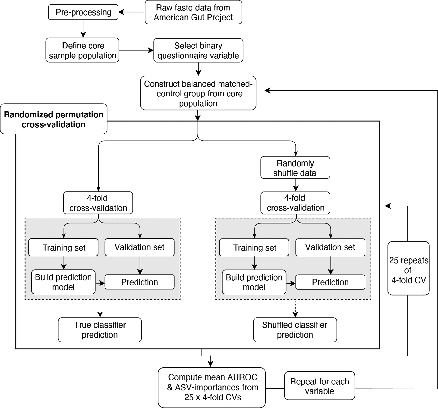
Raw V4 16S rRNA reads were processed using dada2 and samples were filtered and selected as described in the text and Methods to form the ‘core sample population’. Balanced cohorts were constructed for each binary questionnaire variable, and Random Forests analyses were repeated 25 times over 75/25 splits. Concurrently, sample classes were randomly permuted to simulate noise and the same procedure was performed to facilitate empirical P value estimations.

Extended Data Figure 2: Machine learning evaluation of common exclusion criteria and variables for matching.

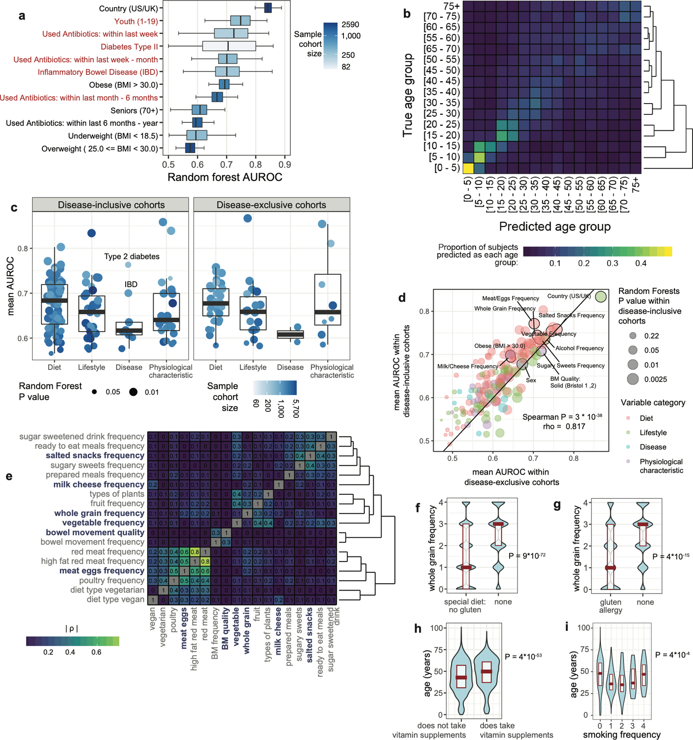
A) Random Forests analysis was performed on binary metadata variables commonly used to shape comparative gut microbiota surveys (N=4,038 subjects). Red labels represent variables chosen for exclusion while blue labels represent included subjects. Center lines represent median values of 100-repeat mean AUROC’s, boxes denote interquartile ranges, and whiskers denote 1.5*interquartile ranges. B) Support vector machine analysis was performed on subjects by age group. Shown is a normalized confusion matrix, averaged across all cross-validation folds. Hierarchical clustering using Euclidean distances with average weighting is shown to the right. C) Random Forests AUROC values for all variables with empirical P < 0.05, shown by variable category. Analysis results for “disease-inclusive” cohorts (with only T2D and IBD removed as per final exclusion criteria, N=5,878) are shown as well as results using only subjects reporting no medical diagnoses of diseases (“disease-exclusive” cohorts, N=2,971). Center lines represent median values of 100-repeat mean AUROC’s, boxes denote interquartile ranges, and whiskers denote 1.5*interquartile ranges. D) Random Forests AUROC values for physiological, lifestyle, and diet variables in subjects reporting no medical diagnoses of diseases (“disease-exclusive” cohorts, N=2,971; x-axis) compared to disease-inclusive cohorts (N=5,878). Outlined in black are representative cohorts for all variables chosen for matching. For frequency-based variables, the frequency categories (e.g. daily, regular) with highest AUROC in the disease-exclusive cohorts are outlined. E) Spearman co-correlation heatmap of all top microbiota-associated variables (those with median AUROC > 0.7 and P < 0.05 by Random Forests). Absolute values of Spearman rho correlation coefficients are shown for each variable pair at their intersections. F) Whole grain consumption frequency between non-celiac subjects reporting no dietary gluten intake (a binary variable that exhibited mean AUROC > 0.7 and P < 0.05 by Random Forests). G) Whole grain consumption frequency between celiac subjects and non-celiac subjects that report no special gluten-free diet (also mean AUROC > 0.7 and P < 0.05). H) Subjects taking vitamin supplements are older than those not taking vitamin supplements. As in F and G, significance assessed by two-sided Mann-Whitney U test. I) Age and smoking frequency display a non-monotonic association. Accordingly, ‘Hoeffding’s D’ statistical test was used to find a significant non-monotonic association between the two variables.

Extended Data Figure 3: Evaluation of Random Forest microbiota association strengths compared to beta diversity assessments and as a function of sample size.

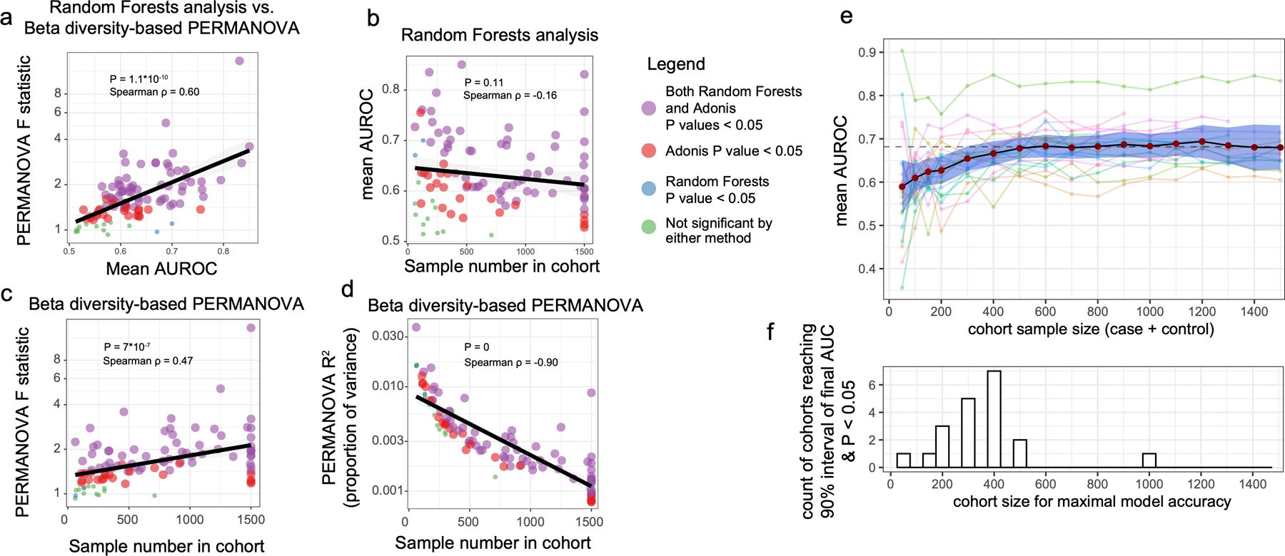
Shown are plots wherein each dot represents results for a single binary cohort representing a single variable including all those listed in Supplementary Table 1. Cohort sizes were capped at 1,500 cases and controls. P values and non-parametric Spearman correlation coefficients are shown in each plot for each comparison. A) Random Forest AUROC values correlate with beta diversity-based PERMANOVA F statistics, and finds significant differences between cases and controls for fewer cohorts than does PERMANOVA. B) Sample size exhibits no significant correlation with Random Forests AUROC values. C) Sample size correlates with PERMANOVA F statistics. D) Sample size correlates strongly with PERMANOVA R² effect size values for each variable. E) From binary and frequency host variables, variables were selected that had n>800 samples and mean AUROC>0.65 (total N=21 host variables). Sample cohorts for each variable were systematically down-sampled by random selection of subjects such that one case-control cohort was constructed with n=50, 100, 150, 200, and then in size increments of 100 until reaching the final cohort size. Mean AUROC values were calculated for each cohort and mean values are represented by red dots with blue depicting 95% confidence interval. F) Cohort size for maximal model accuracy was determined as the first cohort size at which Random Forests empirical P reached a value less than 0.05 and mean AUROC reached a 90% interval of the final AUROC (that of the full cohort).

Extended Data Figure 4: Comparison of microbiota-host variable association strengths between disease-inclusive and disease-exclusive cohorts.

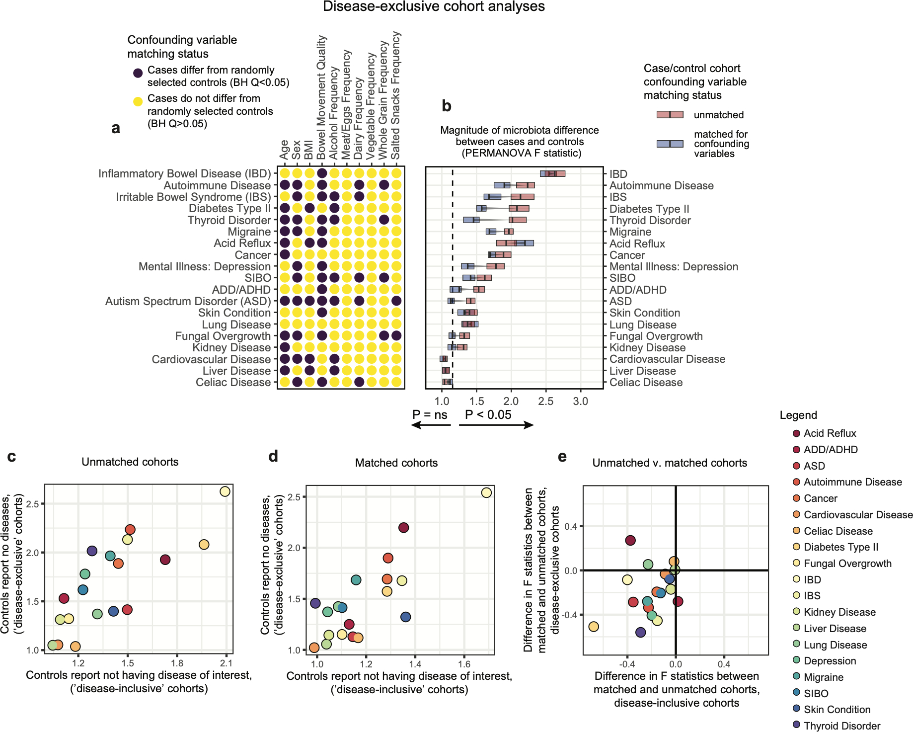
A-B) Differences in PERMANOVA F statistics between matched and unmatched cohorts within disease-exclusive analyses with all subjects reporting medical diagnoses removed, analogous to Figure 2. Subjects in ‘matched’ cohorts were matched for confounding variables shown to differ between cases and controls (purple) in panel A on a per-disease basis. Boxes represent interquartile ranges in F statistics from 25 permuted cohorts per matched/unmatched condition. Center lines within boxes represent median F statistic values. C) F statistics denoting differences between cases and controls for each disease among unmatched (location-only matched) cohorts comparing disease-exclusive to disease-inclusive results. Spearman rho= 0.81, P = 3.2*10⁻⁵. D) F statistics denoting differences between cases and controls for each disease among confounder-matched cohorts comparing disease-exclusive to disease-inclusive results. Spearman rho= 0.64, P = 2.9*10⁻³. E) Concordance in whether matching reduces or increases case-control microbiota differences were examined for disease-inclusive and disease-exclusive results. Differences in F statistics between matched and unmatched cohorts for each disease were calculated. Shown are F statistics differences for disease-inclusive cohorts (x-axis) and disease-exclusive cohorts (y-axis). Chi-square P = 0.0073, assuming random distribution of points across quadrants as the null hypothesis.

Extended Data Figure 5: Machine learning and compositional analyses for diseases before and after confounder matching.

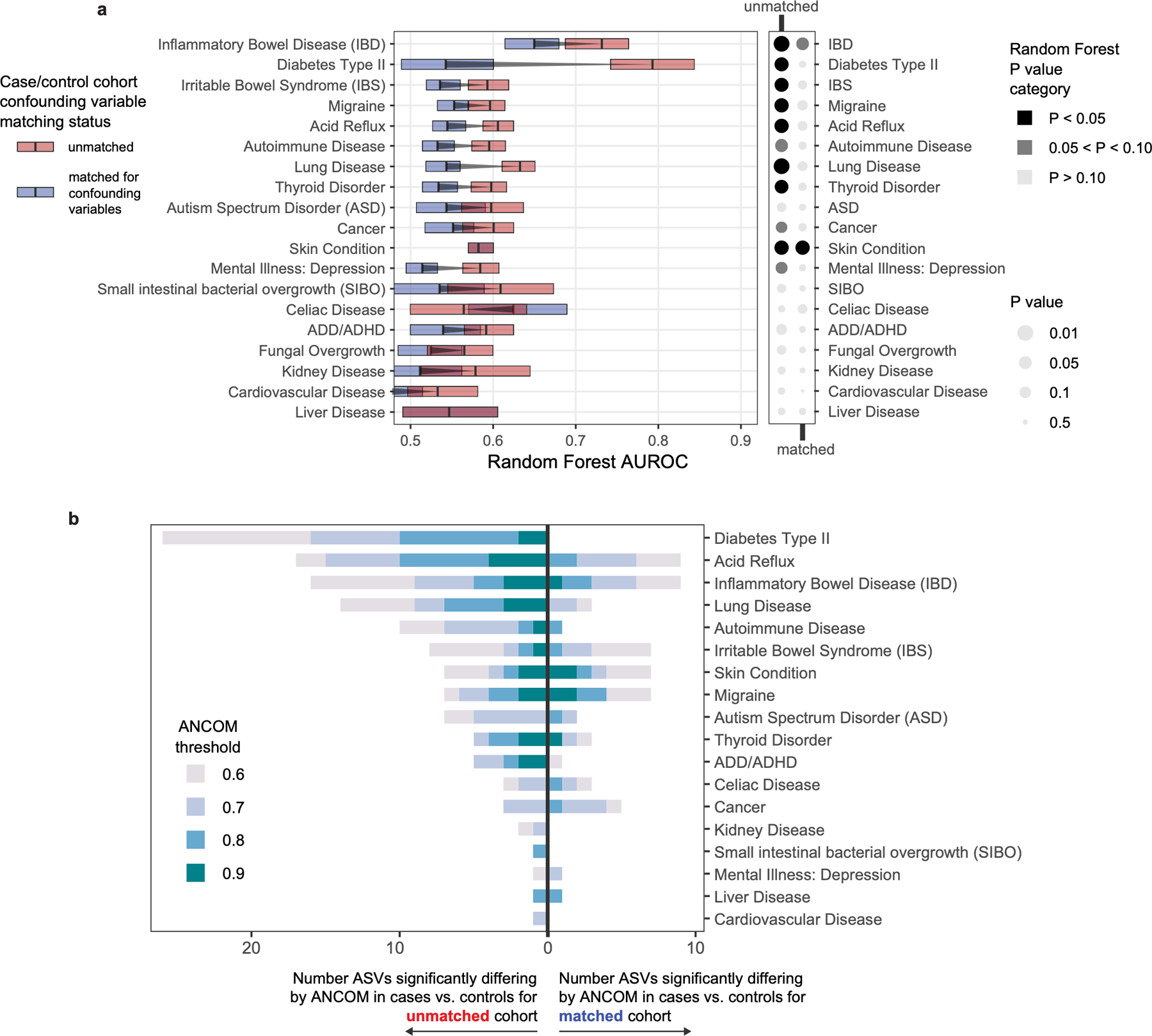
A) Matching cases and controls for key microbiota confounding variables substantially reduces observed microbiota differences between cases and controls, as assessed by machine learning methods. Random Forests analysis was performed as in Figure 2 on location-paired unmatched case control cohorts (red boxes) and case control cohorts matched for confounding variables shown in Figure 2 (blue boxes). Empirical P value significance based on comparison of AUROCs to permuted ‘shuffled’ data was calculated as described in methods. Boxes represent interquartile ranges in 100-repeat mean AUROC values per matched/unmatched condition. Center lines within boxes represent median AUROC values. B) Numbers of differentially abundant ASVs in disease cases versus controls before and after matching cohorts for confounding variables. ANCOM W score thresholds were calculated and ASVs are shown that met each threshold. Notably for type 2 diabetes, 26 ASVs differed significantly before matching, while zero ASVs differed post-matching.

Extended Data Figure 6: Assessment of capacity for statistical methods to correct for mis-matching.

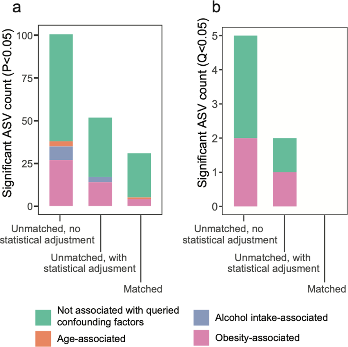
Linear mixed effects analyses were performed as described for Figure 4J. A) Shown are ASVs that passed unadjusted P < 0.05 in the comparison of diabetics to non-diabetic controls via linear mixed effects models, as compared to the more conservative cutoffs shown in Figure 4J (Benjamini-Hochberg Q value < 0.05). B) Shown are ASVs with Benjamini-Hochberg Q value < 0.05 in the comparison of diabetics to non-diabetic controls via linear mixed effects models, with ASVs associated with confounding variables identified by ANCOM as having a W score indicating rejection of the null hypothesis for >80% of log ratio comparisons for that ASV.

Extended Data Figure 7: Validation of confounding effects of host variables in external independent cohorts of type 2 diabetes and metabolic syndrome.

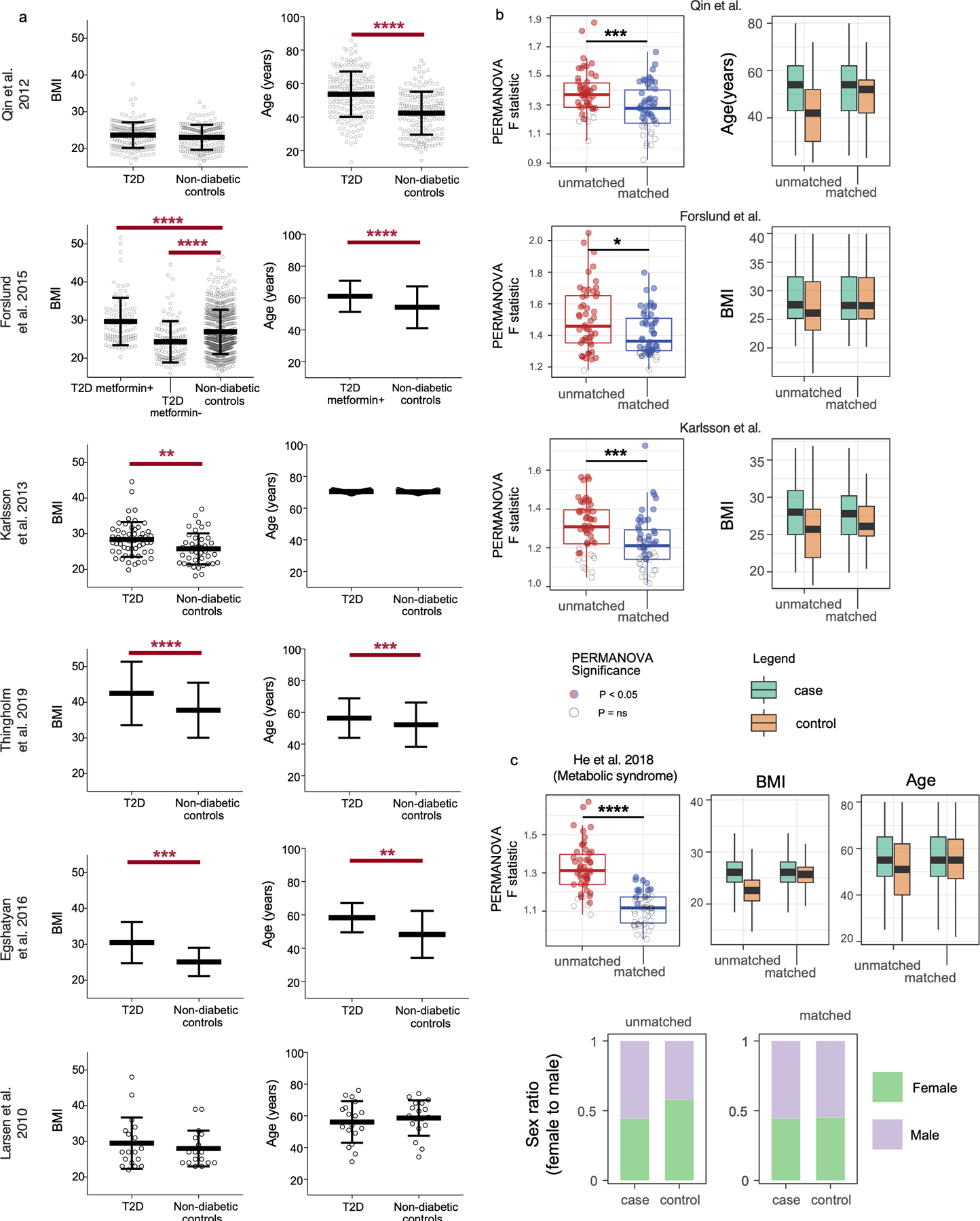
A) Microbiota-associated host variable distributions between cases and controls in prominent type 2 diabetes gut microbiota surveys. Unpaired t-tests were performed where raw data was available. For studies in which raw data was partial or not found, P values reported in each original publication are shown (Forslund et al., Egshatyan et al.). Center lines denote mean and whiskers denote standard deviation. B) Matched and unmatched T2D case-control cohorts were constructed from independent studies shown. Student’s T test was used to compare PERMANOVA F statistic values between randomly selected unmatched cohorts to cohorts that were matched for available confounder metadata (age, BMI, and BMI respectively). Cohort selections were bootstrapped by re-selecting case and control subjects 25 times for both unmatched and matched cohorts. Metformin+T2D were selected for comparison to non-diabetic controls for the study by Forslund et al. Success of matching was assessed using Wilcoxon signed-rank tests and matched cohorts exhibited median Q>0.05 (ns) for each available confounding variable. C) Metabolic syndrome was examined in an external independent study. BMI, age, and sex were found to differ between location-matched (matched by district in Guangdong) subjects and metabolic syndrome cases. Subjects were matched by these variables including district, and F statistics were compared to unmatched (district-only-matched) case-control cohorts. Center lines represent median values, boxes denote interquartile ranges, and whiskers denote 1.5*interquartile ranges. * P ≤ 0.05; ** P ≤ 0.01; *** P ≤ 0.001; **** P ≤ 0.0001

Extended Data Figure 8: Assessment of strength of confounding effects for microbiota-associated confounding host variables.

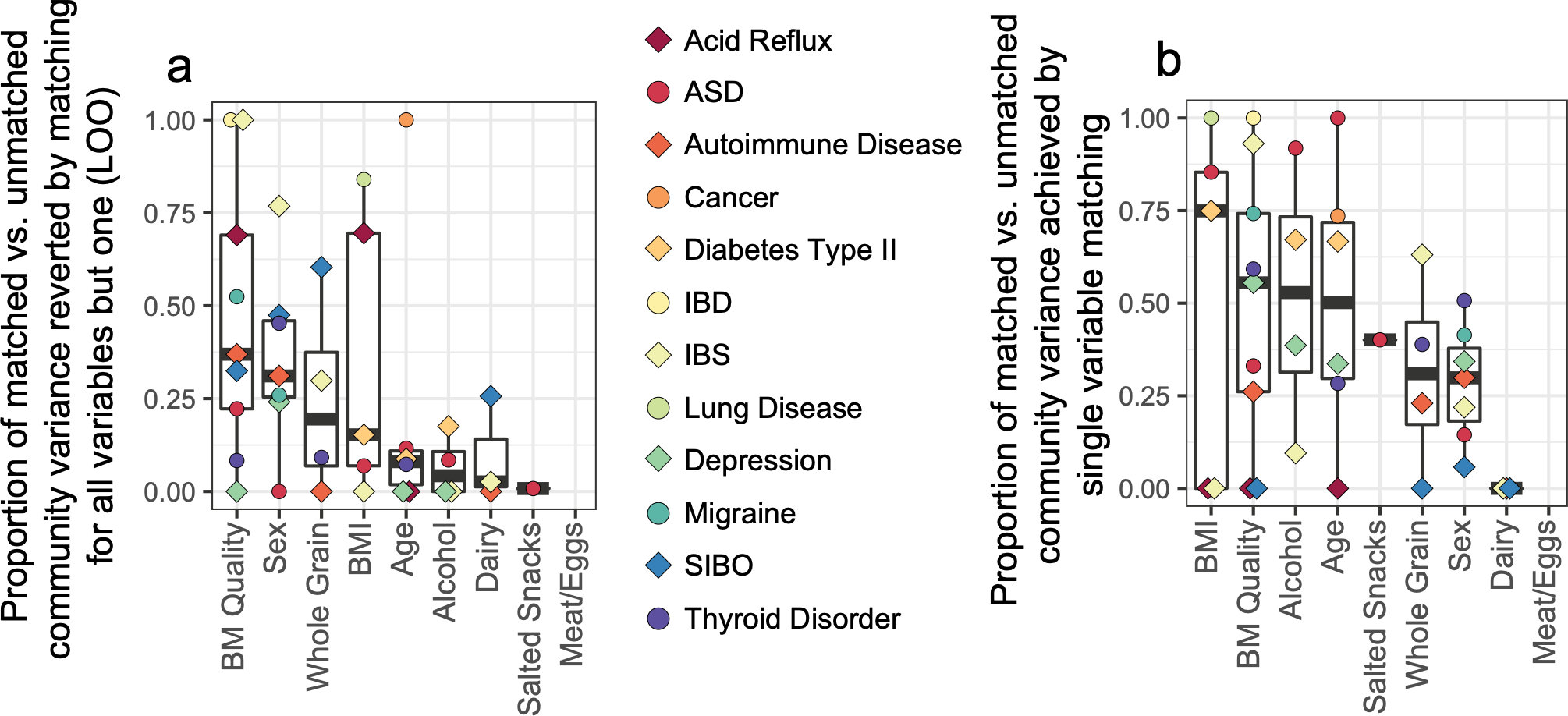
A) Cases and controls were matched for all relevant matching variables except one that was held out (‘leave one out’ [LOO]). The impact of the single variable held out was then assessed by comparing the increase of PERMANOVA F statistic between cases and controls to that of the total change in F statistic from fully matched to unmatched case-control cohorts. Thus, an assessment for the relative independent contribution of each variable to confounding effects in the setting of matching for all other variables was obtained for each variable for each disease. B) Matching by a single variable was performed and resulting F statistics were similarly compared to the difference in F statistics from unmatched to fully matched cohorts, as described in Methods. In A and B, center lines represent median values, boxes denote interquartile ranges, and whiskers denote 1.5*interquartile ranges.

Extended Data Figure 9: Examination of effects of alcohol consumption on the gut microbiota with external validation.

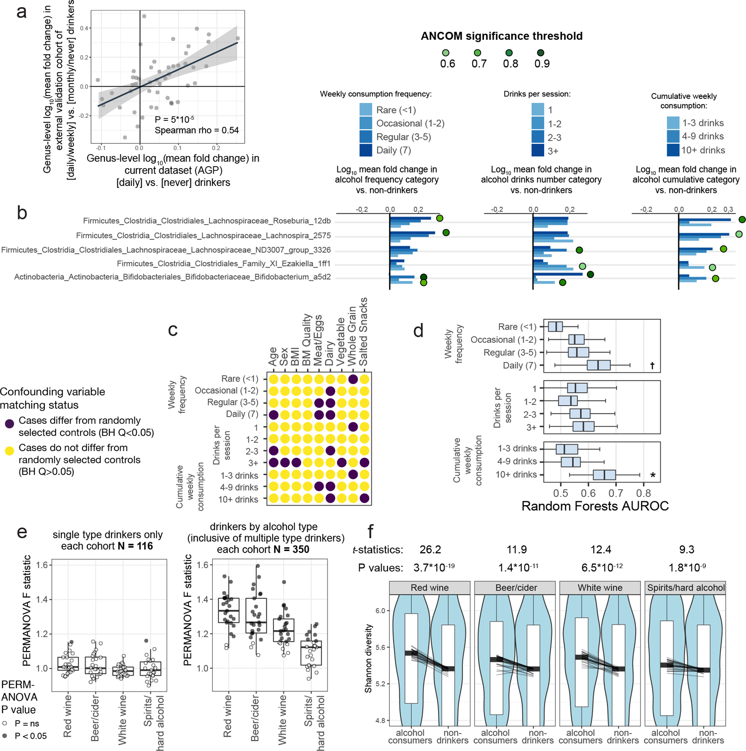
A) ASV abundances were collapsed to the genus level and log₁₀ mean fold changes were calculated between daily versus never drinkers in the AGP dataset (x axis) and compared to log₁₀ mean fold changes in daily/weekly versus monthly/never drinkers in an external validation dataset (y axis). Spearman correlation test P = 10⁻⁴ B) ASVs in differential abundance in all alcohol consumer cohorts compared to matched control non-drinker subjects, by ANCOM. Matched cohorts were constructed by selecting controls matched for all confounding variables and ANCOM was performed. ASVs found to differ significantly between cases and controls are marked by green circles and denoted by their ANCOM threshold. C) Alcohol consumption frequency, number per session, and cumulative weekly consumption are confounded for various microbiota-associated host variables. D) Microbiota covariate association strength as estimated by Random Forests empirical P value tests for alcohol consumption cohorts. Alcohol subjects were matched to never-drinker controls for confounding variables shown in Extended Data Figure 9A and Random Forests analysis was performed as in Figure 2. Bars denote interquartile ranges of AUROCs from 100 repeats. Empirical P=0.0739, P=0.0495. E) Subjects reporting drinking only one type of alcohol (beer/cider, red wine, white wine, or spirits/hard alcohol), were compared to non-drinkers matched for variables shown in (C). Cohort sample sizes were increased when including drinkers who consumed multiple types, and significant median PERMANOVA P values were observed: P=0.004, P=0.007, P=0.021, P=0.076. In D and E, center lines represent median values, boxes denote interquartile ranges, and whiskers denote 1.5*interquartile ranges. F) Alpha diversity was calculated for subjects reporting consumption of each alcohol type (inclusive of those who also drink other types). Lines depict differences in median alpha diversity between cases and controls for each of the 25 re-sampled case-control cohorts. Unadjusted two-sided paired Student’s t-tests were performed. † P ≤ 0.10, *P ≤ 0.05.

Extended Data Figure 10: Bowel movement quality matching and external validation.

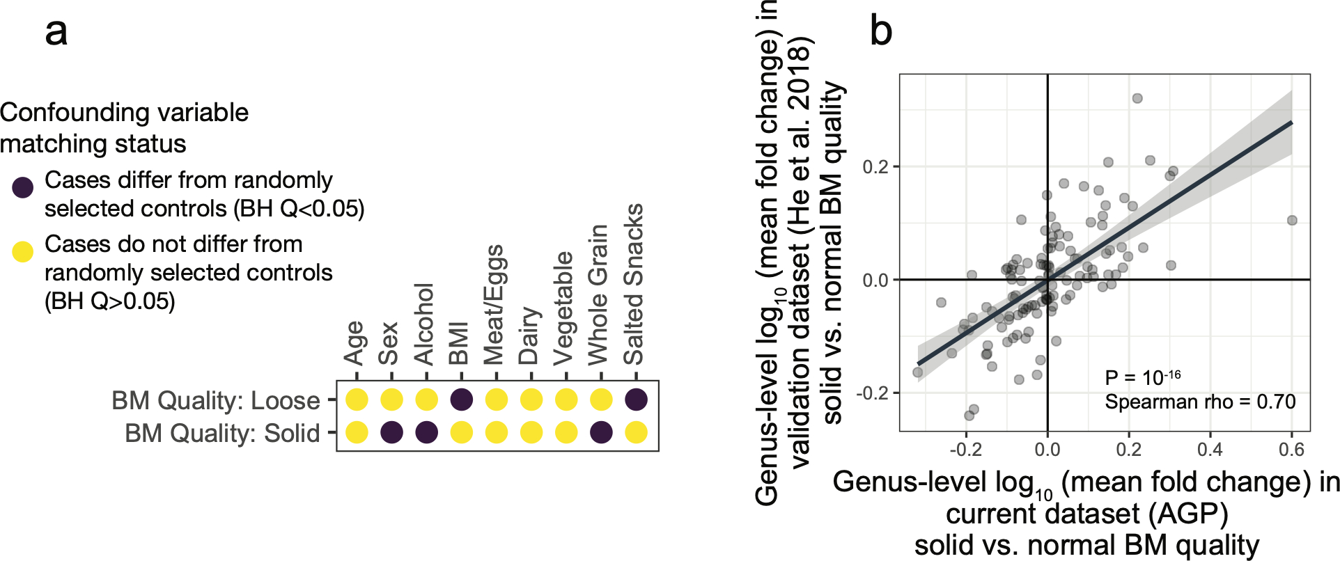
A) Subjects reporting solid or loose bowel movement (BM) quality were compared to subjects reporting normal BM quality in terms of their distribution of microbiota-confouding variables. All BM subject cohorts were thus subsequently matched for sex, alcohol, BMI, whole grain, and salted snack consumption (for Figure 4E–F). B) ASV abundances were collapsed to the genus level and log₁₀ mean fold changes were calculated between solid versus normal BM quality subjects AGP dataset (x axis) and compared to log₁₀ mean fold changes in sold versus normal BM quality subjects in an external validation dataset¹⁵ (y axis). Spearman correlation test P = 10⁻¹⁶

References

- 1.Huttenhower C et al. Structure, function and diversity of the healthy human microbiome. Nature (2012) doi: 10.1038/nature11234. [DOI] [PMC free article] [PubMed] [Google Scholar]
- 2.Falony G et al. Population-level analysis of gut microbiome variation. Science (80-. ). (2016) doi: 10.1126/science.aad3503. [DOI] [PubMed] [Google Scholar]
- 3.Hsiao EY et al. Microbiota modulate behavioral and physiological abnormalities associated with neurodevelopmental disorders. Cell (2013) doi: 10.1016/j.cell.2013.11.024. [DOI] [PMC free article] [PubMed] [Google Scholar]
- 4.Plovier H et al. A purified membrane protein from Akkermansia muciniphila or the pasteurized bacterium improves metabolism in obese and diabetic mice. Nat. Med (2017) doi: 10.1038/nm.4236. [DOI] [PubMed] [Google Scholar]
- 5.Belkaid Y & Hand TW Role of the microbiota in immunity and inflammation. Cell (2014) doi: 10.1016/j.cell.2014.03.011. [DOI] [PMC free article] [PubMed] [Google Scholar]
- 6.Callahan BJ et al. DADA2: High-resolution sample inference from Illumina amplicon data. Nat. Methods (2016) doi: 10.1038/nmeth.3869. [DOI] [PMC free article] [PubMed] [Google Scholar]
- 7.Mcdonald D et al. American Gut : an Open Platform for Citizen Science. 3, 1–28 (2018). [DOI] [PMC free article] [PubMed] [Google Scholar]
- 8.Forslund K et al. Disentangling type 2 diabetes and metformin treatment signatures in the human gut microbiota. Nature 528, 262–266 (2015). [DOI] [PMC free article] [PubMed] [Google Scholar]
- 9.Qin J et al. A metagenome-wide association study of gut microbiota in type 2 diabetes. Nature 490, 55–60 (2012). [DOI] [PubMed] [Google Scholar]
- 10.Thingholm LB et al. Obese Individuals with and without Type 2 Diabetes Show Different Gut Microbial Functional Capacity and Composition. Cell Host Microbe 26, 252–264.e10 (2019). [DOI] [PMC free article] [PubMed] [Google Scholar]
- 11.Mandal S et al. Analysis of composition of microbiomes: a novel method for studying microbial composition. Microb. Ecol. Heal. Dis (2015) doi: 10.3402/mehd.v26.27663. [DOI] [PMC free article] [PubMed] [Google Scholar]
- 12.Larsen N et al. Gut microbiota in human adults with type 2 diabetes differs from non-diabetic adults. PLoS One 5, (2010). [DOI] [PMC free article] [PubMed] [Google Scholar]
- 13.Egshatyan L et al. Gut microbiota and diet in patients with different glucose tolerance. Endocr. Connect 5, 1–9 (2016). [DOI] [PMC free article] [PubMed] [Google Scholar]
- 14.Karlsson FH et al. Gut metagenome in European women with normal, impaired and diabetic glucose control. Nature 498, 99–103 (2013). [DOI] [PubMed] [Google Scholar]
- 15.He Y et al. Regional variation limits applications of healthy gut microbiome reference ranges and disease models. Nature Medicine (2018) doi: 10.1038/s41591-018-0164-x. [DOI] [PubMed] [Google Scholar]
- 16.Gevers D et al. The treatment-naive microbiome in new-onset Crohn’s disease. Cell Host Microbe (2014) doi: 10.1016/j.chom.2014.02.005. [DOI] [PMC free article] [PubMed] [Google Scholar]
- 17.Vich Vila A et al. Gut microbiota composition and functional changes in inflammatory bowel disease and irritable bowel syndrome. Sci. Transl. Med (2018) doi: 10.1126/scitranslmed.aap8914. [DOI] [PubMed] [Google Scholar]
- 18.Lloyd-Price J et al. Multi-omics of the gut microbial ecosystem in inflammatory bowel diseases. Nature (2019) doi: 10.1038/s41586-019-1237-9. [DOI] [PMC free article] [PubMed] [Google Scholar]
- 19.Vujkovic-Cvijin I et al. HIV-associated gut dysbiosis is independent of sexual practice and correlates with noncommunicable diseases. Nat. Commun 11, 2448 (2020). [DOI] [PMC free article] [PubMed] [Google Scholar]
- 20.Llopis M et al. Intestinal microbiota contributes to individual susceptibility to alcoholic liver disease. Gut 65, 830–839 (2016). [DOI] [PubMed] [Google Scholar]
- 21.Ciocan D et al. Bile acid homeostasis and intestinal dysbiosis in alcoholic hepatitis. Aliment. Pharmacol. Ther 48, 961–974 (2018). [DOI] [PubMed] [Google Scholar]
- 22.Dubinkina VB et al. Links of gut microbiota composition with alcohol dependence syndrome and alcoholic liver disease. Microbiome 5, 141 (2017). [DOI] [PMC free article] [PubMed] [Google Scholar]
- 23.Le Roy CI et al. Red Wine Consumption Associated With Increased Gut Microbiota α-diversity in 3 Independent Cohorts. Gastroenterology (2019) doi: 10.1053/j.gastro.2019.08.024. [DOI] [PubMed] [Google Scholar]
- 24.Valles-Colomer M et al. The neuroactive potential of the human gut microbiota in quality of life and depression. Nat. Microbiol (2019) doi: 10.1038/s41564-018-0337-x. [DOI] [PubMed] [Google Scholar]
- 25.Reese AT et al. Using DNA Metabarcoding To Evaluate the Plant Component of Human Diets: a Proof of Concept. mSystems (2019) doi: 10.1128/msystems.00458-19. [DOI] [PMC free article] [PubMed] [Google Scholar]
- 26.Noguera-Julian M et al. Gut Microbiota Linked to Sexual Preference and HIV Infection. EBioMedicine (2016) doi: 10.1016/j.ebiom.2016.01.032. [DOI] [PMC free article] [PubMed] [Google Scholar]
- 27.Amir A et al. Correcting for Microbial Blooms in Fecal Samples during Room-Temperature Shipping. mSystems (2017) doi: 10.1128/msystems.00199-16. [DOI] [PMC free article] [PubMed] [Google Scholar]
- 28.Vujkovic-Cvijin I et al. Dysbiosis of the gut microbiota is associated with HIV disease progression and tryptophan catabolism. Sci. Transl. Med (2013) doi: 10.1126/scitranslmed.3006438. [DOI] [PMC free article] [PubMed] [Google Scholar]
- 29.Deschasaux M et al. Depicting the composition of gut microbiota in a population with varied ethnic origins but shared geography. Nat. Med (2018) doi: 10.1038/s41591-018-0160-1. [DOI] [PubMed] [Google Scholar]
- 30.Yasuda K et al. Biogeography of the intestinal mucosal and lumenal microbiome in the rhesus macaque. Cell Host Microbe (2015) doi: 10.1016/j.chom.2015.01.015. [DOI] [PMC free article] [PubMed] [Google Scholar]
- 31.Cadwell K et al. Virus-Plus-Susceptibility Gene Interaction Determines Crohn’s Disease Gene Atg16L1 Phenotypes in Intestine. Cell (2010) doi: 10.1016/j.cell.2010.05.009. [DOI] [PMC free article] [PubMed] [Google Scholar]
- 32.Zhernakova A et al. Population-based metagenomics analysis reveals markers for gut microbiome composition and diversity. Science (80-. ). (2016) doi: 10.1126/science.aad3369. [DOI] [PMC free article] [PubMed] [Google Scholar]
- 33.Wilck N et al. Salt-responsive gut commensal modulates TH17 axis and disease. Nature (2017) doi: 10.1038/nature24628. [DOI] [PMC free article] [PubMed] [Google Scholar]
- 34.Korem T et al. Bread Affects Clinical Parameters and Induces Gut Microbiome-Associated Personal Glycemic Responses. Cell Metab. (2017) doi: 10.1016/j.cmet.2017.05.002. [DOI] [PubMed] [Google Scholar]
- 35.Ojala M & Garriga GC Permutation tests for studying classifier performance. J. Mach. Learn. Res 11, 1833–1863 (2010). [Google Scholar]
- 36.Barter RL & Yu B Superheat: An R Package for Creating Beautiful and Extendable Heatmaps for Visualizing Complex Data. J. Comput. Graph. Stat (2018) doi: 10.1080/10618600.2018.1473780. [DOI] [PMC free article] [PubMed] [Google Scholar]
- 37.Seidell JC & Halberstadt J The global burden of obesity and the challenges of prevention. Ann. Nutr. Metab (2015) doi: 10.1159/000375143. [DOI] [PubMed] [Google Scholar]
- 38.Palleja A et al. Recovery of gut microbiota of healthy adults following antibiotic exposure. Nat. Microbiol 3, (2018). [DOI] [PubMed] [Google Scholar]
- 39.Pasolli E et al. Accessible, curated metagenomic data through ExperimentHub. Nature Methods (2017) doi: 10.1038/nmeth.4468. [DOI] [PMC free article] [PubMed] [Google Scholar]
Associated Data
This section collects any data citations, data availability statements, or supplementary materials included in this article.