Ensemble Kalman Methods With Constraints

Abstract

Ensemble Kalman methods constitute an increasingly important tool in both state and parameter estimation problems. Their popularity stems from the derivative-free nature of the methodology which may be readily applied when computer code is available for the underlying state-space dynamics (for state estimation) or for the parameter-to-observable map (for parameter estimation). There are many applications in which it is desirable to enforce prior information in the form of equality or inequality constraints on the state or parameter. This paper establishes a general framework for doing so, describing a widely applicable methodology, a theory which justifies the methodology, and a set of numerical experiments exemplifying it.

1. Introduction

1.1. Overview

Kalman filter based methods have been enormously successful in both state and parameter estimation problems. However, a major disadvantage of such methods is that they do not naturally take constraints into account. The ability to constrain a system often has a number of advantages that can play an important role in state and parameter estimation: they can be used to enforce physicality of modeled systems (non-negativity of physical quantities, for example); relatedly they can be used to ensure that computational models are employed only within state and parameter regimes where the model is well-posed; and finally the application of constraints may provide robustness to outlier data. Resulting improvements in algorithmic efficiency and performance, by means of enforcing constraints, has been demonstrated in the recent literature in a diverse set of fields, including process control [1], biomechanics [2], cell energy metabolism [3], medical imaging [4], engine health estimation [5], weather forecasting [6], chemical engineering [7], and hydrology [8]. Within the Kalman filtering literature the need to incorporate constraints is widely recognized and has been addressed in a systematic fashion by viewing Kalman filtering from the perspective of optimization. Indeed this optimization perspective leads naturally to many extensions, and to the incorporation of constraints in particular. Including constraints in Kalman filtering, via optimization, lends itself to an elegant mathematical framework, to a practical computational framework, and has potential in numerous applications. Surveys of the work may be found in the papers of Aravkin, Burke and co-workers [9, 10] and our work in this paper may be viewed as generalizing their perspective to the ensemble setting.

In the probabilistic view of filtering methods, constraints may be introduced by moving beyond the Gaussian assumptions that underpin Kalman methods and imposing constraints through the prior distributions on states and/or parameters. This, however, can create significant computational burden as the resulting distributions cannot be represented in closed form, through a finite number of parameters, in the way that Gaussian distributions can be. Here we circumvent this issue by taking the viewpoint that ensemble Kalman methods constitute a form of derivative-free optimization methodology, eschewing the probabilistic interpretation. The ensemble is used to calculate surrogates for derivatives. With this optimization perspective, constraints may be included in a natural way. Standard ensemble Kalman methods employ a quadratic optimization problem encapsulating relative strengths of belief in the predictions of the model and the data; these optimization problems have explicit analytic solutions. To impose constraints the optimization problem is solved only within the constraint set; when the constraints form a non-empty closed convex set, this constrained optimization problem has a unique solution.

In this introductory section, we give a literature review of existing work in this setting, we describe the contributions in this paper, and we outline notation used throughout.

1.2. Literature Review

Overviews of state estimation using Kalman based methods may be found in [11, 12, 13, 14]. The focus of this article is on ensemble based Kalman methods, introduced by Evensen in [15] and further developed in [16, 11]. The extension of the ensemble Kalman methodology to parameter estimation and inverse problems is overviewed in [17], especially for oil reservoir applications, and in an application-neutral formulation in [18]. Equipping Kalman-based methods with constraints can be desirable for a variety of inter-linked reasons described in the previous subsection: to enforce known physical boundaries in order to improve estimation accuracy; to operationalize filtering of a model which is ill-posed in subsets of its state or parameter space; and to provide robustness to noisy data and outlier events.

In extending the Kalman filter to non-Gaussian settings, a number of methods may be considered. Particle filters provide the natural methodology if propagation of probability distributions is required for state [19] or parameter [20] estimation. In the optimization setting, there are three primary methodologies: the extended Kalman filter, the unscented Kalman filter and the ensemble Kalman filter. The extended Kalman filter is based on linearization of the nonlinear system and therefore needs the computation of derivatives for propagation of the state covariance; this makes them unattractive in high dimensional problems. Unscented and ensemble Kalman filters, on the other hand, can be considered as particle-based methods which are derivative-free. In the unscented Kalman filter, the particles (sigma points) are chosen deterministically and are propagated through the nonlinear system to approximate the covariance, which is then corrected using the Kalman gain to compute the new sigma points. In the ensemble Kalman filter, the particles (ensemble members) are chosen randomly from the initial ensemble and are propagated through the dynamical system and corrected using the Kalman gain without needing to maintain the covariance.

In [21], and more recently in [22], overviews of different ways to impose constraints in linear and nonlinear state estimation are presented. To ensure that the estimates satisfy the constraints, moving horizon based estimators that solve a constrained optimization problem have been proposed [23, 24]. The paper [25] proposed a recursive nonlinear dynamic data reconciliation (RNDDR) approach based on extended Kalman filtering to ensure that state and parameter estimates satisfy the imposed bounds and constraints. The updated state estimates in this method are obtained by solving an optimization problem instead of using the Kalman gain. The resulting covariance calculations are, however, still similar to the Kalman filter: that is, unconstrained propagation and correction involving the Kalman gain, which can affect the accuracy of the estimates. To eliminate this deficiency, [26] proposed a Kullback-Leibler based method to update states and error covariances by solving a convex optimization problem involving conic constraints.

On the other hand, the paper [27] combined the concept of the unscented transformation [28] with the RNDDR formulation. In the prediction step, they propose step sizes to scale sigma points asymmetrically to better approximate the covariance information in the presence of lower and upper bounds. Then, for the update of each sigma point, they solve a constrained optimization problem. One disadvantage of this procedure is that the chosen step sizes for scaling the sigma points can only ensure the bound constraints. The paper [1] also tested various algorithms based on constrained optimization, projection [29] and truncation [5] to enforce bound constraints on unscented Kalman filtering. The paper [30] developed a class of estimators named constrained unscented recursive estimators to address the limitations of the unscented RNDDR method using optimization-based projection algorithms for obtaining sigma points in the presence of convex, non-convex and bound constraints.

As mentioned earlier, since the corrected covariance is used to compute the sigma points, unscented formulations always require enforcing constraints in both propagation and correction/update steps. In contrast, ensemble-based methods only require constraints to be enforced in the update step. In this context, the paper [8] tested projection and accept/reject methods to constrain ensemble members in a post-processing step, after application of the unconstrained ensemble Kalman filter. In the former, they project the updated ensemble members to the feasible space if they violate the constraints and in the latter they enforce the updated ensemble members to obey the constraints by resampling the dynamic and/or data model errors. On the other hand, [31, 32] proposed updating the state estimates in ensemble Kalman filtering by solving a constrained optimization problem while truncating the Gaussian distribution of the initial ensemble. The paper [6] demonstrated how to enforce a physics-based conservation law on an ensemble Kalman filtering based state estimation problem by formulating the filter update as a set of quadratic programming problems arising from a linear data acquisition model subject to linear constraints. Here we develop this body of work on constraining ensemble Kalman techniques, providing a unifying framework with an underpinning theoretical basis.

1.3. Our Contribution

The preceding literature review demonstrates that the imposition of constraints on state and parameter estimation procedures is highly desirable. It also indicates that ensemble Kalman methods offer the most natural context in which to attempt to do this, as extended Kalman methods do not scale well to high dimensional state or parameter space, whilst the unscented filter does not lend itself as naturally to the incorporation of constraints.

In this paper we build on the application-specific papers [8, 6] which demonstrate how to impose a number of particular constraints on ensemble based parameter and state estimation problems respectively. We formulate a very general methodology which is application-neutral and widely applicable, thereby making the ideas in [8, 6] accessible to a wide community of researchers working in inverse problems and state estimation. We also describe a straightforward mathematical analysis which demonstrates that the resulting algorithms are well-defined since they involve the solution of quadratic minimization problems subject to convex constraints at each step of the algorithm; these optimization problems have a unique solution. And finally we showcase the methodology on two applications, one from biomedicine and one from seismology. All of the algorithms discussed are clearly stated in pseudo-code.

Section 2 outlines the ensemble Kalman (EnKF) methodology for state estimation, with and without constraints. In section 3 the same program is carried out for ensemble Kalman inversion (EKI). Section 4 describes the numerical experiments which illustrate the foregoing ideas.

1.4. Notation

Throughout the paper we use $\mathbb{N}$ to denote the positive integers {1, 2, 3,⋯} and ${\mathbb{Z}}^{+}$ to denote the non-negative integers $\mathbb{N}\cup \left\{0\right\}=\{0,1,2,3,\cdots \}$. The matrix I_M denotes the identity on ${ℝ}^M$. We use |⋅| to denote the Euclidean norm, and the corresponding inner-product is denoted ⟨⋅,⋅⟩. A symmetric, square matrix A is positive definite (resp. positive semi-definite) if the quadratic form ⟨u, Au⟩ is positive (resp. non-negative) for all u ≠ 0. By |⋅|_B we denote the weighted norm defined by $|v{|}_B^2=v^{*}{B}^{-1}v$ for any positive-definite B. The corresponding weighted Euclidean inner-product is given by ⟨⋅,⋅⟩_B:= ⟨⋅, B⁻¹⟩. We use ⊗ to denote the outer product between two vectors: (a ⊗ b) = ⟨b, c⟩a.

2. Ensemble Kalman State Estimation

2.1. Filtering Problem

Consider the discrete-time dynamical system with noisy state transitions and noisy observations in the form:

$$\text{Dynamics Model:}{v}_{j+1}=\mathrm{\Psi }\left(v_j\right)+{\xi }_j,j\in {\mathbb{Z}}^{+}$$

$$\text{Data Model:}{y}_{j+1}=H{v}_{j+1}+{\eta }_{j+1},j\in {\mathbb{Z}}^{+}$$

$$\text{Probabilistic Structure:\hspace{1em}}{v}_0~N\left(m_0,C_0\right),{\xi }_j~N(0,\Sigma ),{\eta }_j~N(0,\mathrm{\Gamma })$$

$$\text{Probabilistic Structure:}{v}_0\perp \left\{{\xi }_j\right\}\perp \left\{{\eta }_j\right\}\text{independent}$$

We assume that ${\mathcal{H}}_1$, ${\mathcal{H}}_2$ are finite dimensional Hilbert spaces. Then $v_j\in {\mathcal{H}}_1$,and $\mathrm{\Psi }:{\mathcal{H}}_1\mapsto {\mathcal{H}}_1$ is the state-transition operator. The operator $H:{\mathcal{H}}_1\mapsto {\mathcal{H}}_2$ is the linear observation operator and $y_j\in {\mathcal{H}}_2$. The covariance operators C₀, Σ are assumed to be invertible. The objective of filtering is to estimate the state v_j of the dynamical systems at time J, given the data ${\left\{y_{\mathcal{l}}\right\}}_{\mathcal{l}=1}^j$Remark 2.1. • We may extend the methodology in this paper to the setting where ${\mathcal{H}}_1$, ${\mathcal{H}}_2$ are separable infinite dimensional Hilbert spaces. The covariance operators C₀, Σ are assumed trace-class on ${\mathcal{H}}_1$, and Γ on ${\mathcal{H}}_2$ to ensure that the initial condition v₀ and the noises ξ_J and η_J live in ${\mathcal{H}}_1$, ${\mathcal{H}}_1$ and ${\mathcal{H}}_2$ (respectively) with probability one. The update formulae we derive require operator composition and inversion, together with minimization of quadratic functionals on ${\mathcal{H}}_1$ subject to convex constraints. Provided all of these operations can be carried out, then the methods derived here are well-defined in the general Hilbert space setting. This fact is important because it means that the methods derived have a robustness to mesh refinement and similar procedures arising when the problem of interest is specified via a partial differential equation, or other infinite dimensional problem.

• We restrict attention to linear observation operators H because this leads to solvable quadratic optimization problems within the context of Kalman-based methods. In principle, a non-linear observation operator could be used, but the optimization problems defining the algorithms arising in this paper might not have a unique solution in this setting.

2.2. Ensemble Kalman Filter

The ensemble Kalman filter is a particle-based sequential optimization approach to the state estimation problem. The particles are denoted by ${\left\{v_j^{(n)}\right\}}_{n=1}^N$ and represent a collection of N candidate state estimates at time j. The method proceeds as follows. The state of all the particles at time j + 1 are predicted using the dynamics model to give ${\left\{{\widehat{v}}_{j+1}^{(n)}\right\}}_{n=1}^N$. The resulting empirical covariance of the particles is then used to define the objective function I_filter,_,(v), which encapsulates the model-data compromise. This is minimized in order to obtain the updates ${\left\{v_{j+1}^{(n)}\right\}}_{n=1}^N$ To understand the origin of this optimization perspective on ensemble Kalman methods we argue as follows. In equation (4.10) of [33], it is shown that the data incorporation step of the Kalman filter may be written as a quadratic optimization problem for the state. In equation (4.15) of [33], the ensemble Kalman filter is written by using this quadratic minimization principle with an empirically (from the ensemble) computed covariance.

The prediction step is

$${\widehat{v}}_{j+1}^{(n)}=\mathrm{\Psi }\left(v_j^{(n)}\right)+{\xi }_j^{(n)},n=1,\dots ,N$$ (1a)

$${\widehat{m}}_{j+1}=\frac{1}{N}\sum _{n=1}^N{\widehat{v}}_{j+1}^{(n)}$$ (1b)

$${\widehat{C}}_{j+1}=\frac{1}{N}\sum _{n=1}^N\left({\widehat{v}}_{j+1}^{(n)}-{\widehat{m}}_{j+1}\right){\left({\widehat{v}}_{j+1}^{(n)}-{\widehat{m}}_{j+1}\right)}^T.$$ (1c)

Here we have ${\xi }_j^{(n)}~N(0,\mathrm{\Sigma })$ i.i.d.. Because the empirical covariance contains only N − 1 independent pieces of information, (1c) is sometimes scaled by N − 1 and not N; making this change would lead to no changes in the statements and proofs of all the theorems, and would only affect the definition of covariance within the algorithms.

Let $\mathcal{R}\left({\widehat{C}}_{j+1}\right)$ denote the range of ${\widehat{C}}_{j+1}$ The update step is then

$$v_{j+1}^{(n)}=\underset{v}{\text{argmin}}{I}_{\text{filter,j,n}}(v)$$ (2)

where

$$I_{\text{filter, }j,n}(v):=\{\begin{array}{ll}\frac{1}{2}{\left|y_{j+1}^{(n)}-Hv\right|}_{\mathrm{\Gamma }}^2+\frac{1}{2}{\left|v-{\widehat{v}}_{j+1}^{(n)}\right|}^2\hfill & \text{ if }v-{\widehat{v}}_{j+1}^{(n)}\in \mathcal{R}\left({\widehat{C}}_{j+1}\right).\hfill \\ \infty \hfill & \text{ otherwise. }\hfill \end{array}$$ (3)

It can be useful to rewrite the objective function for the optimization problem in an equivalent and more standard form for input to software:

$$\{\begin{array}{ll}\frac{1}{2}{v}^T\left(H^T{\mathrm{\Gamma }}^{-1}H+{\widehat{C}}_{j+1}^{-1}\right)v-{\left({\widehat{C}}_{j+1}^{-1^T}{\widehat{v}}_{j+1}^{(n)}+H^T{\mathrm{\Gamma }}^{-1^T}{y}_{j+1}^{(n)}\right)}^{T}v\hfill & \text{ if }v-{\widehat{v}}_{j+1}^{(n)}\in \mathcal{R}\left({\widehat{C}}_{j+1}\right).\hfill \\ \infty \hfill & \text{ otherwise. }\hfill \end{array}$$

The $y_{j+1}^{(n)}$ are either identical to the data Y_J+1, or found by perturbing it randomly.

Note that ${\widehat{C}}_{j+1}$ is an operator of rank at most N − 1, and thus can only be invertible when N − 1 is larger than the dimension of ${\mathcal{H}}_1$. For moderate- and high-dimensional systems, it is often impractical to satisfy this condition. However, the minimizing solution can be found by regularizing ${\widehat{C}}_{j+1}$ by addition of ∈I for ∈ > 0, deriving the update equations and then letting ∈ → 0. We give the resulting formulae, and then justify them immediately afterwards, in the following subsubsection. Alternatively it is possible to directly seek a solution in $\mathcal{R}\left({\widehat{C}}_{j+1}\right)$, which is a subspace of dimension N − 1; this is done in the subsequent subsubsection.

2.2.1. Formulation In The Original Variables

The well-known Kalman update formulae arising from solution of the minimization problem (2), (3) are as follows:

$$S_{j+1}=H{\widehat{C}}_{j+1}{H}^T+\mathrm{\Gamma }$$ (4a)

$$K_{j+1}={\widehat{C}}_{j+1}{H}^T{S}_{j+1}^{-1}\text{\hspace{1em}(Kalman Gain)}$$ (4b)

$$y_{j+1}^{(n)}=y_{j+1}+s{\eta }_{j+1}^{(n)},n=1,\dots ,N$$ (4c)

$$v_{j+1}^{(n)}=\left(I-K_{j+1}H\right){\widehat{v}}_{j+1}^{(n)}+K_{j+1}{y}_{j+1}^{(n)},n=1,\dots ,N$$ (4d)

Here ${\eta }_j^{(n)}~N(0,\mathrm{\Gamma })$ i.i.d. and the constant s takes value 0 or 1. When s = 1 the $y_{j+1}^{(n)}$ are referred to as perturbed observations. The choice s = 1 is made to ensure the correct statistics of the updates in the linear Gaussian setting when a probabilistic viewpoint is taken, and more generally to introduce diversity into the ensemble procedure when an optimization viewpoint is taken.

Derivation of the formulae may be found in [33]. In brief the formulae arise from completing the square in the objective function I _filter,j,n(·) and then applying the Sherman–Morrison formula to rewrite the updates in the data space rather than state space; the latter is advantageous in many applications where ${\mathcal{H}}_2$ has dimension much smaller than ${\mathcal{H}}_1$.

We summarize with the following pseudo-code:

An equivalent formulation of the minimization problem is now given by means of a penalized Lagrangian approach to incorporate the property that the solution of the optimization problem lies in the range of the empirical covariance. The perspective is particularly useful when further constraints are imposed on the solution of the optimization problem.

Theorem 2.2. Suppose that the dimensions of ${\mathcal{H}}_1$ and ${\mathcal{H}}_2$ are finite. Let j be in ${\mathbb{Z}}^{+}$ and 1 ≤ n ≤ N. Define $y^{\prime }=y_{j+1}^{(n)}-H{\widehat{v}}_{j+1}^{(n)}$ Then the update formulae (4), which follow from the minimization problem (2), (3), may be given alternatively as

$$v_{j+1}^{(n)}={\widehat{v}}_{j+1}^{(n)}+\underset{\left(a,v^{\prime }\right)\in \mathcal{A}}{\text{argmin}}\left(\frac{1}{2}{\left|y^{\prime }-H{v}^{\prime }\right|}_{\mathrm{\Gamma }}^2+\frac{1}{2}\langle a,v^{\prime }\rangle \right)$$ (5)

where $\mathcal{A}=\left\{\left(a,v^{\prime }\right)\in {\mathcal{H}}_1\times {\mathcal{H}}_1:{\widehat{C}}_{j+1}a=v^{\prime }\right\}$ and the argmin is projected from the pair (a,v’) onto the v^′ coordinate only. Moreover $v_{j+1}^{(n)}=\underset{ϵ\to 0}{\text{lim}}{v}_{ϵ}$ with

$$v_{ϵ}=\underset{v\in {\mathcal{H}}_1}{\text{argmin}}\left(\frac{1}{2}{\left|y_{j+1}^{(n)}-Hv\right|}_{\mathrm{\Gamma }}^2+\frac{1}{2}{\left|{\widehat{v}}_{j+1}^{(n)}-v\right|}_{{\widehat{C}}_{ϵ}}^2\right)$$ (6)

and $\widehat{C}={\widehat{C}}_{j+1}+\in I$.

proof. For notational convenience denote $\widehat{C}={\widehat{C}}_{j+1}$. The objective function I_filter,,(v) appearing in (3) is infinite if and only if $v-{\widehat{v}}_{j+1}^{(n)}$ is in the range of $\widehat{C}$. Thus, since the range of $\widehat{C}$ is non-empty, we may confine minimization to the set of $\left(a,v^{\prime }\right)\in \mathcal{A}$. Note that $\widehat{C}$ is in general not invertible, as it has rank N − 1,which may be less than the dimension of ${\mathcal{H}}_1$. The set $\mathcal{A}$ thus comprises all v^′ in the range of $\widehat{C}$(a convex set) and, for each such v^′ the set of a solving $\widehat{C}a=v^{\prime }$; such an a is unique up to translations in the null-space of $\widehat{C}$. Thus $\mathcal{A}$ is a convex set. Notice that, for such pairs $\left(a,v^{\prime }\right)\in \mathcal{A}$, $\langle a,v^{\prime }\rangle ={\left|v^{\prime }\right|}_{\widehat{C}}^2$ with v^′ lying in the range of the operator $\widehat{C}$. Although the element a is uniquely defined only up to translations in the nullspace of $\widehat{C}$, such translations do not change the value of the inner product ⟨a, v^′⟩. The restriction of $\widehat{C}$ over the constraint set is positive definite which means that the quadratic objective function, now depending only on v^′, is strongly convex. Therefore the problem has a unique solution and its Lagrangian is written as:

$$\mathcal{L}\left(v^{\prime },a,\lambda \right)=\frac{1}{2}{\left|y^{\prime }-H{v}^{\prime }\right|}_{\mathrm{\Gamma }}^2+\frac{1}{2}\langle a,v^{\prime }\rangle +\langle \lambda ,\widehat{C}a-v^{\prime }\rangle$$

To express optimality conditions compute the derivatives and set them to zero:

$$\begin{gathered} -H^T{\mathrm{\Gamma }}^{-1}\left(y^{\prime }-H{v}^{\prime }\right)+\frac{1}{2}a-\lambda =0, \\ \frac{1}{2}{v}^{\prime }+\widehat{C}\lambda =0, \\ {v}^{\prime }-\widehat{C}a=0. \end{gathered}$$

The last two equations imply that $\widehat{C}(2\lambda +a)=0$. Thus we set $\lambda =-\frac{1}{2}a$ and drop the second equation, replacing the first by

$$-H^T{\mathrm{\Gamma }}^{-1}\left(y^{\prime }-H\widehat{C}a\right)+a=0.$$

Solving the resulting equation for a gives

$$a={\left(H^T{\mathrm{\Gamma }}^{-1}H\widehat{C}+I\right)}^{-1}{H}^T{\mathrm{\Gamma }}^{-1}{y}^{\prime }.$$

From this formula it follows that

$$\begin{gathered} v_{j+1}^{(n)}={\widehat{v}}_{j+1}^{(n)}+v^{\prime } \\ ={\widehat{v}}_{j+1}^{(n)}+\widehat{C}a \\ ={\widehat{v}}_{j+1}^{(n)}+\widehat{C}{\left(H^T{\mathrm{\Gamma }}^{-1}H\widehat{C}+I\right)}^{-1}{H}^T{\mathrm{\Gamma }}^{-1}{y}^{\prime } \\ ={\widehat{v}}_{j+1}^{(n)}+\widehat{C}{\left(H^T{\mathrm{\Gamma }}^{-1}H\widehat{C}+I\right)}^{-1}{H}^T{\mathrm{\Gamma }}^{-1}\left(y_{j+1}^{(n)}-H{\widehat{v}}_{j+1}^{(n)}\right). \end{gathered}$$

If we define

$$K=\widehat{C}{\left(H^T{\mathrm{\Gamma }}^{-1}H\widehat{C}+I\right)}^{-1}{H}^T{\mathrm{\Gamma }}^{-1}$$ (8)

then we see that

$$v_{j+1}^{(n)}=(I-KH){\widehat{v}}_{j+1}^{(n)}+K{y}_{j+1}^{(n)}.$$ (9)

This is precisely the form of the ensemble Kalman update, and to complete the proof of the first part of the theorem it remains to show that this defintion of K agrees with the formulae given in (4); this amounts to verifying the identity

$${\left(H^T{\mathrm{\Gamma }}^{-1}H\widehat{C}+I\right)}^{-1}{H}^T{\mathrm{\Gamma }}^{-1}=H^T{\left(H\widehat{C}{H}^T+\mathrm{\Gamma }\right)}^{-1}.$$ (10)

To verify this we start from the matrix identity

$${\left(H^T{\mathrm{\Gamma }}^{-1}H\widehat{C}+I\right)}^{-1}\left(H^T{\mathrm{\Gamma }}^{-1}H\widehat{C}{H}^T+H^T\right)=H^T$$

noting that it may be factored to write

$${\left(H^T{\mathrm{\Gamma }}^{-1}H\widehat{C}+I\right)}^{-1}\left(H^T{\mathrm{\Gamma }}^{-1}\right)\left(H\widehat{C}{H}^T+\mathrm{\Gamma }\right)=H^T.$$

Inverting $\left(H\widehat{C}{H}^T+\mathrm{\Gamma }\right)$ on the right gives the desired identity (10).

We now study the alternative representation of the minimization problem (2), (3), by (6). We first note that $H^T{\mathrm{\Gamma }}^{-1}H+{\widehat{C}}_{ϵ}^{-1}$ is strictly positive definite and hence the related quadratic function is strongly convex. As a consequence we have existence and uniqueness of the solution, and the optimality condition becomes,

$$\left(H^T{\mathrm{\Gamma }}^{-1}H+{\widehat{C}}_{ϵ}^{-1}\right)v_{ϵ}=H^T{\mathrm{\Gamma }}^{-1}{y}_{j+1}^{(n)}+{\widehat{C}}_{ϵ}^{-1}{\widehat{v}}_{j+1}^{(n)}.$$

Then if we apply Woodbury matrix identity we obtain

$$v_{ϵ}=\left({\widehat{C}}_{ϵ}-{\widehat{C}}_{ϵ}{H}^T{\left(H{\widehat{C}}_{ϵ}{H}^T+\mathrm{\Gamma }\right)}^{-1}H{\widehat{C}}_{ϵ}\right)\left(H^T{\mathrm{\Gamma }}^{-1}{y}_{j+1}^{(n)}+{\widehat{C}}_{ϵ}^{-1}{\widehat{v}}_{j+1}^{(n)}\right).$$

Note that the matrix multiplying ${\widehat{v}}_{j+1}^{(n)}$is

$$\left({\widehat{C}}_{ϵ}-{\widehat{C}}_{ϵ}{H}^T{\left(H{\widehat{C}}_{ϵ}{H}^T+\mathrm{\Gamma }\right)}^{-1}H{\widehat{C}}_{ϵ}\right){\widehat{C}}_{ϵ}^{-1}=\left(I-{\widehat{C}}_{ϵ}{H}^T{\left(H{\widehat{C}}_{ϵ}{H}^T+\mathrm{\Gamma }\right)}^{-1}H\right)$$

and that the matrix multiplying $y_{j+1}^{(n)}$ is

$$\begin{gathered} \left({\widehat{C}}_{ϵ}-{\widehat{C}}_{ϵ}{H}^T{\left(H{\widehat{C}}_{ϵ}{H}^T+\mathrm{\Gamma }\right)}^{-1}H{\widehat{C}}_{ϵ}\right)H^T{\mathrm{\Gamma }}^{-1} \\ ={\widehat{C}}_{ϵ}{H}^T\left(I-{\left(H{\widehat{C}}_{ϵ}{H}^T+\mathrm{\Gamma }\right)}^{-1}H{\widehat{C}}_{ϵ}{H}^T\right){\mathrm{\Gamma }}^{-1} \\ ={\widehat{C}}_{ϵ}{H}^T{\left(H{\widehat{C}}_{ϵ}{H}^T+\mathrm{\Gamma }\right)}^{-1}\mathrm{\Gamma }{\mathrm{\Gamma }}^{-1} \\ ={\widehat{C}}_{ϵ}{H}^T{\left(H{\widehat{C}}_{ϵ}{H}^T+\mathrm{\Gamma }\right)}^{-1} \end{gathered}$$

so that

$$v_{ϵ}=\left(I-{\widehat{C}}_{ϵ}{H}^T{\left(H{\widehat{C}}_{ϵ}{H}^T+\mathrm{\Gamma }\right)}^{-1}H\right){\widehat{v}}_{j+1}^{(n)}+{\widehat{C}}_{ϵ}{H}^T{\left(H{\widehat{C}}_{ϵ}{H}^T+\mathrm{\Gamma }\right)}^{-1}{y}_{j+1}^{(n)}.$$

Finally, as A↦A⁻¹ is continuous over the set of invertible matrices, letting ϵ → 0 gives:

$$\underset{ϵ\to 0}{\text{lim}}{v}_{ϵ}=\left(I-K_{j+1}H\right){\widehat{v}}_{j+1}^{(n)}+K_{j+1}{y}_{j+1}^{(n)}$$

which concludes the proof.

2.2.2. Formulation In Range Of The Covariance

The minimization problem for each individual particle has a solution which, when suitably shifted, lies in the range of the empirical covariance. This allows us to seek the solution of the minimization problem as a linear combination of a given set of vectors, and to minimize over the scalars which define this linear combination. This reformulation of the optimization problem is widely employed in a variety of applications, such as weather forecasting, where the number of ensemble members N is much smaller than the dimension of the data space; this is because the inversion of S to form the Kalman gain K takes place in the data space.

In order to implement the minimization in the N dimensional subspace we note that I _filter,j,n(v) is infinite unless

$$v-{\widehat{v}}_{j+1}^{(n)}={\widehat{C}}_{j+1}a$$

for some $a\in {ℝ}^n$ _.From the structure of ${\widehat{C}}_{j+1}$ given in (1c) it follows that

$$v={\widehat{v}}_{j+1}^{(n)}+\frac{1}{N}\sum _{m=1}^N{b}_m{e}^{(m)},e^{(m)}:={\widehat{v}}_{j+1}^{(m)}-{\widehat{m}}_{j+1}.$$ (11)

Here each unknown parameter $b_m\in ℝ$ and $b:={\left\{b_m\right\}}_{m=1}^N$, is the unknown vector to be determined. This form for v follows from the fact that which in turn implies that

$${\widehat{C}}_{j+1}=\frac{1}{N}\sum _{m=1}^N{e}^{(m)}\otimes e^{(m)}$$ (12)

which in turn implies that

$${\widehat{C}}_{j+1}a=\frac{1}{N}\sum _{m=1}^N{b}_m{e}^{(m)}.$$ (13)

Note that the unknown vector b depends on n as we need to solve the constrained minimization problem for each of the particles, indexed by n = 1,…, N; we have suppressed the dependence of b on n for notational simplicity.

The expression (11) for v in terms of the e^(m) can be substituted into (3) to obtain a functional J_filter,j,n(b) to be minimized over $b\in {ℝ}^N$, because v is an affine function of b. Equation (11) may be written in compact form as

$$v={\widehat{v}}_{j+1}^{(n)}+Bb$$ (14)

where B is the linear mapping from ${ℝ}^N$ into ${\mathcal{H}}_1$ defined by

$$Bb:=\frac{1}{N}\sum _{m=1}^N{b}_m{e}^{(m)}.$$

We now identify J_filter,j,n(b). We note that (13) is solved by taking

$$b_m=\langle e^{(m)},a\rangle .$$

Although a is not unique, the non-uniqueness stems only from translations in the nullspace of ${\widehat{C}}_{j+1}$. Translations do affect the values taken by the b_m, but do not affect the vector v given by (14) because they result in changes to b which are in the null-space of B. Furthermore, for any such solution, independently of which a is chosen,

$$\frac{1}{2}{\left|v-{\widehat{v}}_{j+1}^{(n)}\right|}_{{\widehat{C}}_{j+1}}^2=\frac{1}{2}\langle a,{\widehat{C}}_{j+1}a\rangle =\frac{1}{2N}\sum _{m=1}^N{b}_m^2.$$

Using this and (14) in the definition of I_filterj,n(v) we obtain

$$J_{\text{filter},j,n}(b)=I_{\text{filter},j,n}\left({\widehat{v}}_{j+1}^{(n)}+Bb\right)$$

and hence, from (3),

$$J_{\text{filter, }j,n}(b):=\frac{1}{2}{\left|y_{j+1}^{(n)}-H{\widehat{v}}_{j+1}^{(n)}-HBb\right|}_{\mathrm{\Gamma }}^2+\frac{1}{2N}|b{|}^2$$ (15a)

$$=\frac{1}{2}{b}^T\left(B^T{H}^T{\mathrm{\Gamma }}^{-1}HB+\frac{1}{N}I\right)b-{\left(B^T{H}^T{\mathrm{\Gamma }}^{-1}\left(y_{j+1}^{(n)}-H{\widehat{v}}_{j+1}^{(n)}\right)\right)}^{T}b+\text{const}.$$ (15b)

Once b is determined it may be substituted back into (14) to obtain the solution to the minimization problem.

The preceding considerations also yield the following result, concerning the unconstrained Kalman minimization problem; its proof is a corollary of the more general Theorem 2.4 from the next subsection, which includes constraints in the minimization problem.

Corollary 2.3. Suppose that the dimensions of ${\mathcal{H}}_1$ and ${\mathcal{H}}_2$ are finite. Given the prediction (1a), the unconstrained Kalman update formulae may be found by minimizing J_filter,j,n (b) from (15) with respect to b and substituting into (14).

We summarize the ensemble Kalman state estimation algorithm, using minimization over the vector b, in the following pseudo-code:

2.3. Constrained Ensemble Kalman Filter

In this subsection we introduce linear equality and inequality constraints on the state variable into the ensemble Kalman filter. We make prediction according to (1), and then incorporate data by solving the minimization problem (3) subject to the additional constraints

$$Fv\text{ =}f\text{,}$$ (16a)

$$Gv\preccurlyeq g.$$ (16b)

Here F and G are linear mappings which, respectively, take the state v into the number of equality and inequality constraints; the notation ≼ denotes inequality componentwise.

2.3.1. Formulation In The Original Variables

The preceding considerations lead to the following algorithm for ensemble Kalman filtering subject to constraints. The existence of a solution to the constrained minimization follows from Theorem 2.4 below.

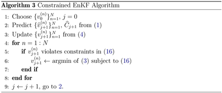
2.3.2. Formulation In Range Of The Covariance

The linear constraints (16) can be rewritten in terms of the vector b, by means of (14), as follows:

$$FBb=f-F{\widehat{v}}_{j+1}^{(n)},$$ (17a)

$$GBb\preccurlyeq g-G{\widehat{v}}_{j+1}^{(n)}.$$ (17b)

We may thus predict and then optimize the objective function J_filter,j,n (b),given by (15), subject to the constraints (17). Implementation of this leads to following algorithm for ensemble Kalman filtering subject to constraints:

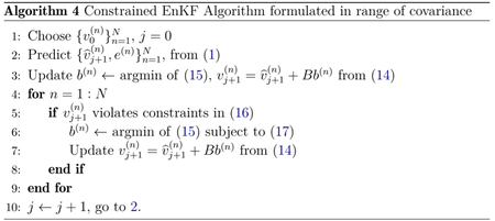
Justification for the use of this algorithm, working in the constrained space parameterized by b, is a consequence of the following:

Theorem 2.4. Suppose that the dimensions of ${\mathcal{H}}_1$ and ${\mathcal{H}}_2$ are finite. The problem of finding $v_{j+1}^{(n)}$ as the minimizer of I_filterj,n(v) subject to the constraints (16) is equivalent to finding b to minimize J_{filter, J,n} (b) subject to the constraints (17) and then using (14) to find $v_{j+1}^{(n)}$ from b. Furthermore, both of these constrained minimization problems have a unique solution provided that the constraint sets are non-empty.

Proof. For notational convenience set $\widehat{v}={\widehat{v}}_{j+1}^{(n)}$, $y=y_{j+1}^{(n)}$, $y^{\prime }=y-H\widehat{v}$, $\widehat{C}={\widehat{C}}_{j+1}$ and ${\widehat{C}}_{ϵ}={\widehat{C}}_{j+1}+ϵI$.

Denote

$$\begin{gathered} v^{*}=\underset{v^{\prime }}{\text{argmin}}\frac{1}{2}{\left|y^{\prime }-H{v}^{\prime }\right|}_{\mathrm{\Gamma }}^2+\frac{1}{2}\langle a,v^{\prime }\rangle \\ \text{subject to\hspace{1em}}•\widehat{C}a=v^{\prime } \\ •F{v}^{\prime }=f-F\widehat{v} \\ •G{v}^{\prime }\preccurlyeq g-G\widehat{v} \end{gathered}$$ (18)

$$\begin{gathered} v_{ϵ}=\underset{v}{\text{argmin}}\frac{1}{2}|y-Hv{|}_{\mathrm{\Gamma }}^2+\frac{1}{2}|v-\widehat{v}{|}_{{\widehat{C}}_{ϵ}}^2 \\ \text{subject to\hspace{1em}}•Fv=f \\ •Gv\preccurlyeq g \end{gathered}$$ (19)

and

$$J(v)=\frac{1}{2}|y-Hv{|}_{\mathrm{\Gamma }}^2+\frac{1}{2}|v-\widehat{v}{|}_{\widehat{C}}^2$$

$$J_{ϵ}(v)=\frac{1}{2}|y-Hv{|}_{\mathrm{\Gamma }}^2+\frac{1}{2}|v-\widehat{v}{|}_{{\widehat{C}}_{ϵ}}^2$$

The part of the statement of Theorem 2.4 concerning existence of a minimizer is a consequence of the Lemma 2.5 stated and proved below. The second part, concerning the equivalence of minimization over b and over v (or v^′) was shown in equations (11)–(15). This concludes the proof.

Notice that in the following lemma, the variables v_ϵ, $\widehat{v}$, and v^* are analogous to $v_{j+1}^{(n)}$, ${\widehat{v}}_{j+1}^{(n)}$, and the minimizer over v^′ from (5), respectively.

Lemma 2.5. Suppose that the constraint sets of (18) and (19) are non empty, then v^* exists and is unique and for all ϵ> 0,v_ϵ exists and is unique. Furthermore $\underset{ϵ\to 0}{\text{lim}}{v}_{ϵ}=\widehat{v}+v^{*}$

Proof. The proof is broken into two parts. In the first we prove existence and uniqueness of a solution by using the idea that the constraint relating a and v^′ renders the problem convex. In the second part of the proof we study the ∈ → 0 limit of the regularized solution, extracting convergent subsequences through compactness, and demonstrating that they converge to the desired limit. To prove existence and uniqueness of the solution of (18), notice that it can be reformulated as

$$\begin{gathered} \underset{v^{\prime }}{\text{ argmin}}J\left(\widehat{v}+v^{\prime }\right) \\ \text{subject to\hspace{1em}}•\widehat{C}a=v^{\prime } \\ •F{v}^{\prime }=f-F\widehat{v} \\ •G{v}^{\prime }\preccurlyeq g-G\widehat{v} \end{gathered}$$

and that the restriction of $\widehat{C}$ over its range is strictly positive definite. Hence J is a strongly convex function being minimized over a nonempty closed convex set. From standard theory v^* exists and is unique. Then as ${\widehat{C}}_{ϵ}$ is strictly positive definite, the same type of arguments provide existence and uniqueness v_∈.

Now we prove the second part of the lemma. We note that $\widehat{v}+v^{*}$ matches the constraints of (19). It follows that for all ϵ > 0, $J_{ϵ}\left(v_{ϵ}\right)\le J_{ϵ}\left(\widehat{v}+v^{*}\right)$. Then let us prove that $J_{ϵ}\left(\widehat{v}+v^{*}\right)\underset{ϵ\to 0}{\to }J\left(\widehat{v}+v^{*}\right)$. First denote by λ₁ ≤⋯≤λ_N−1 the strictly positive eigenvalues of $\widehat{C}$(recall that $\widehat{C}$ is symmetric positive semidefinite and that $\text{rank}(\widehat{C})$ almost surely). Hence ${\widehat{C}}_{ϵ}^{-1}={\sum }_{k=1}^{N-1}\frac{1}{{\lambda }_k+ϵ}{a}_k{a}_k^T+{\sum }_{k=N}^{\text{dim}\left({\mathcal{H}}_1\right)}\frac{1}{ϵ}{a}_k{a}_k^T$ where the a_k’s are the eigenvectors of $\widehat{C}$ (the first and second sums respectively gather the vectors of the range and of the nullspace of $\widehat{C}$). As v^* lies in the range of $\widehat{C}$, it holds that ${\left|v^{*}+\widehat{v}-\widehat{v}\right|}_{{\widehat{C}}_{ϵ}}^2={\left|v^{*}\right|}_{{\widehat{C}}_{ϵ}}^2={\sum }_{k=1}^{N-1}\frac{1}{{\lambda }_k+ϵ}{\left(a_k^T{v}^{*}\right)}^2$ Now as the a_k’s do not depend on ∈, by letting ∈ tending to zero, this quantity will tend to

$$\sum _{k=1}^{N-1}\frac{1}{{\lambda }_k}{\left(a_k^T{v}^{*}\right)}^2={\left|v^{*}\right|}_{\widehat{C}}^2={\left|v^{*}+\widehat{v}-\widehat{v}\right|}_{\widehat{C}}^2.$$

Therefore it holds that $J_{ϵ}\left(\widehat{v}+v^{*}\right)\underset{ϵ\to 0}{\to }J\left(\widehat{v}+v^{*}\right)$. From this we deduce that there exists δ > 0 such that for all 0 < ∈ < δ, $J_{ϵ}\left(v_{ϵ}\right)\le J\left(\widehat{v}+v^{*}\right)+1$ Then set $w_{ϵ}=v_{ϵ}-\widehat{v}=w_{ϵ}^0+w_{ϵ}^1$ where $w_{ϵ}^0$ lies in the nullspace of $\widehat{C}$ and $w_{ϵ}^1$ in its range (recall that for a symmetric matrix nullspace and range are orthogonal) and see that $J_{ϵ}\left(v_{ϵ}\right)=\frac{1}{2}{\left|y^{\prime }-H{w}_{ϵ}\right|}_{\mathrm{\Gamma }}^2+\frac{1}{2}{\left|w_{ϵ}\right|}_{{\widehat{C}}_{ϵ}}^2$. It holds that $\frac{1}{2}{\left|w_{ϵ}\right|}_{{\widehat{C}}_{ϵ}}^2\le J_{ϵ}\left(v_{ϵ}\right)\le J\left(\widehat{v}+v^{*}\right)+1$ for ∈ sufficiently small. Furthermore ${\left|w_{ϵ}\right|}_{{\widehat{C}}_{ϵ}}^2{\widehat{C}}_{ϵ}={\left|w_{ϵ}^0\right|}_{{\widehat{C}}_{ϵ}}^2+{\left|w_{ϵ}^1\right|}_{{\widehat{C}}_{ϵ}}^2=\frac{1}{ϵ}{\left|w_{ϵ}^0\right|}^2+{\left|w_{ϵ}^1\right|}_{{\widehat{C}}_{ϵ}}^2$, and since this quantity is bounded from above we deduce that $w_{ϵ}^0\underset{ϵ\to 0}{\to }0$ and that $w_{ϵ}^1$ is bounded. Let ${\left({ϵ}_m\right)}_{m\in \mathbb{N}}$ be a sequence of positive real numbers such that ${ϵ}_m\underset{m\to \infty }{\to }0$, and from the preceding extract a converging subsequence (denoted ${\left({ϵ}_m\right)}_{m\in \mathbb{N}}$ for simplicity) such that ${\left(w_{{ϵ}_m}^1\right)}_{m\in \mathbb{N}}$ converges to a limit denoted w*. As $w_{{ϵ}_m}^1$ lies in $\mathcal{R}(\widehat{C})$, we can use the eigenvalue decomposition of $\widehat{C}$ to show that ${\left|w_{{ϵ}_m}^1\right|}_{{\widehat{C}}_{{ϵ}_m}}^2\underset{m\to \infty }{\to }{\left|w^{*}\right|}_{\widehat{C}}^2$. This limiting identity, and the fact that $w_{ϵ}^0$ has limit 0, may be used to establish the first equality within the following chain of equalities and inequalities:

$$\begin{gathered} J\left(\widehat{v}+w^{*}\right)=\underset{m\to \infty }{\text{lim}}\frac{1}{2}{\left|y^{\prime }-H{w}_{{ϵ}_m}\right|}_{\Gamma }^2+\frac{1}{2}{\left|w_{{ϵ}_m}^1\right|}_{{\widehat{C}}_{{ϵ}_m}}^2\le \underset{m\to \infty }{\text{lim}}{J}_{{ϵ}_m}\left(v_{{ϵ}_m}\right) \\ \le \underset{m\to \infty }{\text{lim}}{J}_{{ϵ}_m}\left(\widehat{v}+v^{*}\right)=J\left(\widehat{v}+v^{*}\right). \end{gathered}$$

Now note that w* matches all the constraints of (18). Indeed $w_{{ϵ}_m}^1$ lies in the range of $\widehat{C}$ which is a closed space, also $v_{{ϵ}_m}-\widehat{v}=w_{{ϵ}_m}^0+w_{{ϵ}_m}^1\underset{m\to \infty }{\to }{w}^{*}$.It is a clear that $v_{{ϵ}_m}-\widehat{v}$ matches the equality and inequality constraints of (18) for all m and hence passing to the limit we have that w* satisfies the equalities and inequalities.

From the uniqueness of the minimizer of (18) we have that w^* is equal to v^*. In particular this means that v^* is the unique cluster point of the original sequence ${\left(w_{{ϵ}_m}^1\right)}_{m\in \mathbb{N}}$. Since the original sequence was arbitrarily chosen, we conclude that $\underset{ϵ\to 0}{\text{lim}}{v}_{ϵ}=\widehat{v}+v^{*}$ Remark 2.6. Notice that the proof remains true if we take general convex inequalities. We simply need the constrained sets to be closed and convex; however we have restricted to linear equality and inequality constraints for simplicity and because these arise most often in practice.

3. Ensemble Kalman Inversion

3.1. Inverse Problem

In this section we show how a generic inverse problem may be formulated as a partially observed dynamical system. This enables the machinery from the preceding section 2 to be used to solve inverse problems.

We are interested in the inverse problem of finding $u\in {\mathcal{H}}_1$ from $y\in {\mathcal{H}}_2$ where

$$y=G(u)+\eta ,\eta ~N(0,\mathrm{\Gamma }).$$

Time does not appear (explicitly) in this equation (although G may involve solution of a time-dependent differential equation, for example). In order to use the ideas from the previous section, we introduce a new variable w = G(u) and rewrite the equation as

$$\begin{gathered} w=G(u), \\ y=w+\eta . \end{gathered}$$

The key point about writing the equation this way is that the data y is now linearly related to the variable v = (u, w)^T and now we may apply the ideas of the previous section to the model by introducing the following dynamical system, taking y_j+1 = y as the given data:

$$\begin{gathered} u_{j\text{ + 1}}\text{ = }{u}_j, \\ {w}_{j+1}=G\left(u_j\right), \\ {y}_{j+1}=w_{j+1}+{\eta }_{j+1}. \end{gathered}$$

If we introduce the new variables

$$v={(u,w)}^T,\mathrm{\Psi }(v)={(u,G(u))}^T$$ (20a)

$$H=[0,I],H^{\perp }=[I,0],$$ (20b)

and write v_j = (u_j, w_j)^T, we may write the dynamical system in the form

$$v_{j+1}=\mathrm{\Psi }\left(v_j\right)$$ (21a)

$$y_{j+1}=H{v}_{j+1}+{\eta }_{j+1},$$ (21b)

which is exactly in the same form as in the previous section. We note that

$$Hv=w,H^{\perp }v=u.$$

3.2. Ensemble Kalman Inversion

The prediction step and the Kalman gain are defined as in (3), and the solution of the optimization problem is given by (4). We now simplify these formulae using the specific structure on Ψ, v, H arising in the inverse problem and given in (20); this results in block form vectors and matrices. First we note that

$${\widehat{C}}_{j+1}=\left[\begin{array}{cc}{C}_{j+1}^{uu}& C_{j+1}^{uw}\\ {\left(C_{j+1}^{uw}\right)}^T& C_{j+1}^{ww}\end{array}\right],{\overline{v}}_{j+1}=\left(\begin{array}{c}{\overline{u}}_{j+1}\\ {\overline{w}}_{j+1}\end{array}\right).$$

Here

$${\overline{u}}_{j+1}=\frac{1}{N}\sum _{n=1}^N{u}_j^{(n)},{\overline{w}}_{j+1}=\frac{1}{N}\sum _{n=1}^{N}G\left(u_j^{(n)}\right):={\overline{G}}_j$$

and

$$\begin{gathered} C_{j+1}^{uw}=\frac{1}{N}\sum _{n=1}^N\left(u_j^{(n)}-{\overline{u}}_{j+1}\right)\otimes \left(G\left(u_j^{(n)}\right)-{\overline{G}}_j\right), \\ {C}_{j+1}^{ww}=\frac{1}{N}\sum _{n=1}^N\left(G\left(u_j^{(n)}\right)-{\overline{G}}_j\right)\otimes \left(G\left(u_j^{(n)}\right)-{\overline{G}}_j\right), \\ {C}_{j+1}^{uu}=\frac{1}{N}\sum _{n=1}^N\left(u_j^{(n)}-{\overline{u}}_{j+1}\right)\otimes \left(u_j^{(n)}-{\overline{u}}_{j+1}\right). \end{gathered}$$

The covariance $C_{j+1}^{ww}$ denotes the empirical covariance of the ensemble in data space, $C_{j+1}^{uu}$ denotes the empirical covariance of the ensemble in space of the unknown u, and $C_{j+1}^{uw}$ denotes the empirical cross-covariance from data space to the space of the unknown.

Noting that $S_{j+1}={\left(C_{j+1}^{ww}+\mathrm{\Gamma }\right)}^{-1}$ we obtain

$$K_{j+1}=\left(\begin{array}{c}{C}_{j+1}^{uw}{\left(C_{j+1}^{ww}+\mathrm{\Gamma }\right)}^{-1}\\ C_{j+1}^{ww}{\left(C_{j+1}^{ww}+\mathrm{\Gamma }\right)}^{-1}\end{array}\right).$$ (22)

Combining equation (22) with the update equation within (4) it follows that

$${\left\{v_j^{(n)}\right\}}_{n=1}^N\to {\left\{v_{j+1}^{(n)}\right\}}_{n=1}^N$$

and

$${\left\{H^{\perp }{v}_j^{(n)}\right\}}_{n=1}^N\to {\left\{H^{\perp }{v}_{j+1}^{(n)}\right\}}_{n=1}^N$$

and hence that

$$u_{j+1}^{(n)}=H^{\perp }{v}_{j+1}^{(n)}=u_j^{(n)}+C_{j+1}^{uw}{\left(C_{j+1}^{ww}+\mathrm{\Gamma }\right)}^{-1}\left(y_{j+1}^{(n)}-G\left(u_j^{(n)}\right)\right).$$

Thus we have derived the EKI update formula:

$$u_{j+1}^{(n)}=u_j^{(n)}+C_{j+1}^{uw}{\left(C_{j+1}^{ww}+\mathrm{\Gamma }\right)}^{-1}\left(y_{j+1}^{(n)}-G\left(u_j^{(n)}\right)\right).$$ (23)

We note also that

$$w_{j+1}^{(n)}=G\left(u_j^{(n)}\right)+C_{j+1}^{ww}{\left(C_{j+1}^{ww}+\mathrm{\Gamma }\right)}^{-1}\left(y_{j+1}^{(n)}-G\left(u_j^{(n)}\right)\right).$$ (24)

However $w_{j+1}^{(n)}$ is not needed to update the state and so plays no role in this unconstrained EKI algorithm. (It may be used, however, to impose constraints on observation space, as discussed in the next subsection.)

In summary we have derived the following algorithm for solution of the unconstrained inverse problem:

3.3. Ensemble Kalman Inversion With Constraints

3.3.1. Formulation In The Original Variables

We now consider imposing constraints on the optimization step arising in ensemble Kalman inversion. As in the unconstrained case we do this by formulating the problem as a special case of the partially observed dynamical system, subject to constraints, from the previous section.

To this end we formulate the constraints in the space of the unknown and the data as follows:

$$F^{u}u=f^u,$$ (25a)

$$F^{w}w=f^w,$$ (25b)

$$G^{u}u\preccurlyeq g^u,$$ (25c)

$$G^{w}w\preccurlyeq g^w.$$ (25d)

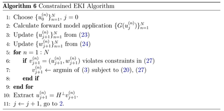
The algorithm proceeds by predicting according to equation (1), and then optimizing (3), all using the specific structure (20), and with the optimization subject to the constraints (25), written in the notation of the general Kalman updating formulae in (27), detailed below; in particular the rewrite (27) of the constraints expresses everything in terms of the variable v. We may summarize the constraints as follows, to allow direct application of the ideas of the previous section. To this end define

$$F=\left(\begin{array}{c}{F}^u{H}^{\perp }\\ F^{w}H\end{array}\right)=\left(\begin{array}{cc}{F}^u& 0\\ 0& F^w\end{array}\right)$$ (26a)

$$G=\left(\begin{array}{c}{G}^u{H}^{\perp }\\ G^{w}H\end{array}\right)=\left(\begin{array}{cc}{G}^u& 0\\ 0& G^w\end{array}\right)$$ (26b)

$$f=\left(\begin{array}{l}{f}^u\hfill \\ f^w\hfill \end{array}\right),g=\left(\begin{array}{l}{g}^u\hfill \\ g^w\hfill \end{array}\right).$$ (26c)

Then the constraints (25) may be written as

$$Fv=f,$$ (27a)

$$Gv\preccurlyeq g.$$ (27b)

See Algorithm 6 for the resulting pseudo-code.

3.3.2. Formulation In Range Of The Covariance

We describe an alternative way to approach the derivation of the EKI update formulae. We apply Theorem 2.4 with the specific structure (20), (27) arising from the dynamical system used in EKI. To this end we define

$$J_{\text{filter},j,n}(b):=\frac{1}{2}{\left|y_{j+1}^{(n)}-G\left(u_j^{(n)}\right)-B^{w}b\right|}_{\mathrm{\Gamma }}^2+\frac{1}{2N}|b{|}^2$$ (28a)

$$=\frac{1}{2}{b}^T\left({\left(B^w\right)}^T{\mathrm{\Gamma }}^{-1}{B}^w+\frac{1}{N}I\right)b-{\left({\left(B^w\right)}^T{\mathrm{\Gamma }}^{-1}\left(y_{j+1}^{(n)}-G\left(u_j^{(n)}\right)\right)\right)}^{T}b+\text{const.}$$ (28b)

where b is the vector of N scalar weights b_m and

$$B^{u}b=\frac{1}{N}\sum _{m=1}^N{b}_m\left(u_j^{(m)}-{\overline{u}}_j\right),$$ (29a)

$$B^{w}b=\frac{1}{N}\sum _{m=1}^N{b}_m\left(G\left(u_j^{(m)}\right)-{\overline{G}}_j\right),$$ (29b)

$$Bb=\left(\begin{array}{c}{B}^{u}b\\ B^{w}b\end{array}\right).$$ (29c)

Once this quadratic form has been minimized with respect to b then the update formula (11) gives

$$u_{j+1}^{(n)}=u_j^{(n)}+\frac{1}{N}\sum _{m=1}^N{b}_m\left(u_j^{(m)}-{\overline{u}}_j\right),$$ (30a)

$$w_{j+1}^{(n)}=G\left(u_j^{(n)}\right)+\frac{1}{N}\sum _{m=1}^N{b}_m\left(G\left(u_j^{(m)}\right)-{\overline{G}}_j\right).$$ (30b)

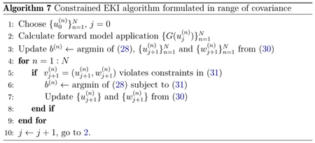
Note that the vector {b_m} depends on the particle label n; as in the previous section, we have suppressed this dependence for notational convenience. We may now impose linear equality and inequality constraints on both u and w = G(u) (i.e. in parameter and data spaces) and minimize (28) subject to these constraints. To be more specific if we impose the constraints (27) expressed in the variable b:

$$FBb=f-F{\widehat{v}}_{j+1}^{(n)},$$ (31a)

$$GBb\preccurlyeq g-G{\widehat{v}}_{j+1}^{(n)}.$$ (31b)

Here F, G, f and g are given by (26), B is defined by (29) and

$${\widehat{v}}_{j+1}^{(n)}=\left(\begin{array}{c}{u}_j^{(n)}\\ G\left(u_j^{(n)}\right)\end{array}\right).$$

See Algorithm 7 for the resulting pseudo-code.

Remark 3.1. As in the previous section, the result holds true for general convex inequality constraints; the linear case is considered for simplicity of exposition, and because it is most frequently arising in practice.

Remark 3.2. The EKI algorithm, with or without constraints, has the following invariant subspace property: define $\mathcal{A}=\text{span}{\left(u_0^{(n)}\right)}_{n\in \{1,\cdots ,N\}}$, then for all J in {0, …, J} and for all n in {1,…, N}, then the $u_j^{(n)}$ defined by the three algorithms in this section all lie in $\mathcal{A}$. This is a direct consequence of writing the update formulae in terms of b and noting (30).

We can now state a result analogous to Theorem 2.4, and with proof that is a straightforward corollary of that result, using the specific structure (20):

Theorem 3.3. Suppose that the dimensions of ${\mathcal{H}}_1$ and ${\mathcal{H}}_2$ are finite. Suppose also that the specific structure (20) is applied. The problem of finding $u_{j+1}^{(n)}$ from the minimizer of I_{filter, J,n}(v), defined in (3) and subject to the constraint (25), is equivalent to finding b that minimizes (28), subject to (31), and then using (30) to find $u_{j+1}^{(n)}$ from b. Furthermore, both of these constrained minimization problems have a unique solution provided that the constraint sets are non-empty.

4. Numerical Results

This section contains numerical results which demonstrate the benefits of imposing constraints on ensemble Kalman methods. Subsection 4.1 concerns an application of state estimation (using EnKF) in biomedicine, using real patient data, whilst subsection 4.2 concerns an application of inversion (using EKI) in seismology and employs simulated data. When comparing results from the two experiments, recall that iterations of EKI correspond to an algorithmic dynamics intended to converge to a single distribution (over ensemble members) on the parameters for which we invert, whereas iterations of EnKF correspond to the incorporation of new data at every physical measurement time, and thus the distribution (over ensemble members) is not necessarily expected to converge as the iteration progresses. In both applications, minimizations were performed in MATLAB using the default interior-point method (fmincon) through the general quadratic programming function, quadprog.

4.1. State Estimation

Here we present an application of the constrained EnKF to the tracking and forecasting of human blood glucose levels. We use self-monitoring data collected by an individual with Type 2 Diabetes. We use the “P1” data set described by Albers et al. in [34]; this dataset includes measurements of blood glucose and consumed nutrition, and is publicly available on physionet.org. For more information on the data, and on an unconstrained data assimilation approach using the unscented Kalman filter, see [34]. We model the glucose-insulin system with the ultradian model proposed by [35]. The primary state variables are the glucose concentration, G, the plasma insulin concentration, I_p, and the interstitial insulin concentration, I_i; these three state variables are augmented with a three stage delay (h₁, h₂, h₃) which encodes a non-linear delayed hepatic glucose response to plasma insulin levels. The resulting ordinary differential equations have the form:

$$\frac{d{I}_p}{dt}=f_1(G)-E\left(\frac{I_p}{V_p}-\frac{I_i}{V_i}\right)-\frac{I_p}{t_p}$$ (32a)

$$\frac{d{I}_i}{dt}=E\left(\frac{I_p}{V_p}-\frac{I_i}{V_i}\right)-\frac{I_i}{t_i}$$ (32B)

$$\frac{dG}{dt}=f_4\left(h_3\right)+m_G(t)-f_2(G)-f_3\left(I_i\right)G$$ (32c)

$$\frac{d{h}_1}{dt}=\frac{1}{t_d}\left(I_p-h_1\right)$$ (32d)

$$\frac{d{h}_2}{dt}=\frac{1}{t_d}\left(h_1-h_2\right)$$ (32e)

$$\frac{d{h}_3}{dt}=\frac{1}{t_d}\left(h_2-h_3\right)$$ (32f)

Here (t) represents a known rate of ingested carbohydrates, f₁(G) represents the rate of glucose-dependent insulin production, f₂(G) represents insulin-independent glucose utilization, f₃(I_i) G represents insulin-dependent glucose utilization and f₄(h₃) represents delayed insulin-dependent hepatic glucose production; the functional forms of these parameterized processes can be found in the appendix, along with a description of model parameters.

In the EnKF setting, we write u = [I_p, I_i, G, h₁, h₂, h₃], and use (32) to define F such that

$$\frac{du}{dt}=F(u,t,\theta ),$$

Where θ contains model parameters. We then extend the state vector in order to perform joint parameter estimation: v = [u, R_g]^T.

For the purposes of this paper, the function (t) may be viewed as known; it is determined from data describing meals consumed by the patient. Since insulin (I_p and I_i) and delay variables (h₁, h₂, and h₃) are not measured, whilst glucose is measured, we define the measurement operator to be H = [0, 0, 1, 0, 0, 0, 0]. The discrete time forward model is obtained by integrating the deterministic model in (32) between consecutive measurement time-points and applying an identity map to R_g. Because these time-points may not be equally spaced, and because the time-dependent forcings (meals) will differ in different time-intervals, this leads to a map of the form

$$v_{j+1}={\mathrm{\Psi }}_j\left(v_j\right).$$

This is a slight departure from the methodology outlined in section 2, where Ψ does not depend on J (autonomous dynamics) but is a straightforward extension which the reader can easily provide.

We present EnKF results from a single patient’s data when run with and without constraints (Algorithms 1 and 3 respectively). We performed joint state-parameter estimation, augmenting the state with parameter R_g (see Appendix for details of where this parameter appears) and adding identity-map dynamics for parameter R_g. The following constraints were imposed:

$$\left[\begin{array}{c}0.01\\ 0.01\\ 2000\\ 0.01\\ 0.01\\ 0.01\\ 0\end{array}\right]\preccurlyeq v\preccurlyeq \left[\begin{array}{c}10000\\ 10000\\ 40000\\ 10000\\ 10000\\ 10000\\ 1000000\end{array}\right]$$ (33)

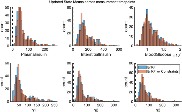
Figure 1 compares the overall distribution of updated state means over time when running EnKF with and without these state constraints. While individual particles in this experiment often violated the constraints, the overall updated means did not. Nevertheless, enforcement of lower-bound constraints shifts up the state distribution slightly. Note that upper bound constraints were never violated in this experiment.

Figure 1.

The distribution of mean state updates when running EnKF with and without inequality constraints. Black vertical lines denote lower bound state constraints.

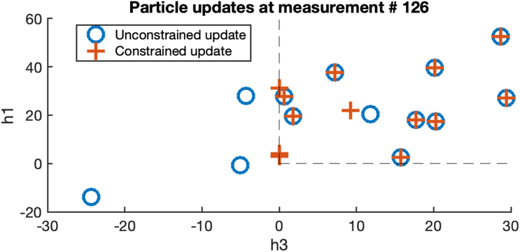
Figure 2 shows a two-dimensional state projection of updated particles at a given time step before and after applying the constrained optimization. Note that particles may additionally violate constraints in unplotted dimensions—this explains why one particle whose unconstrained update appears to live within the constraints is in fact differently updated under the constrained optimization. Time step 126 was selected for illustrative purposes, and was the measurement event in which particles most often violated the constraints.

Figure 2.

Particle updates at a given time-step (here, measurement 126) are shown using a traditional Kalman gain versus using the constrained optimization. The black lines denote lower bound constraints on the states h₁ and h₃.

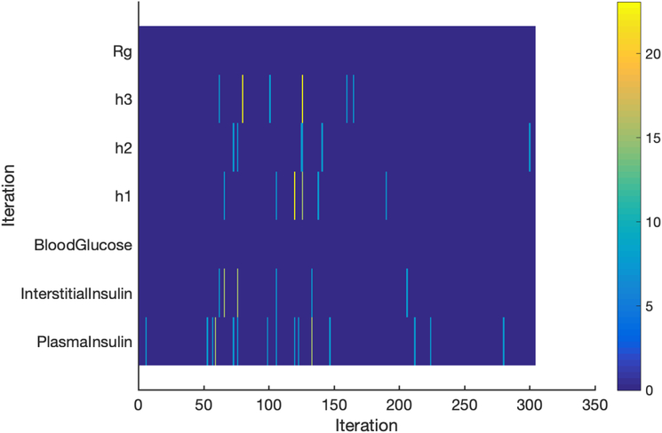
Figure 3 depicts the overall frequency of constraint violations. We observe that the the measured state (blood glucose) never violated a constraint, nor did the inferred parameter R_g. However, other model states did often violate constraints, and up to 30% (4/13) of particles simultaneously violated the constraints at a single time-step.

Figure 3.

Percentage map of the constraint violations, where each lower-bound constraint is represented by a row. At each iteration, the percentage of particles that violated a constraint is color-coded, with yellow representing the largest proportion of constraint violations.

By adding constraints, we ensure that all the simulations which constitute the ensemble method are biologically plausible.

4.2. Inverse Problem

Here we present application of the constrained EKI in seismology. We study near-surface site characterization in which we invert for the shear wave velocity profile of the geomaterials in the earth shallow crust, using downhole array data. For forward modeling, we consider a semi-discrete form of the following wave equation in a horizontally stratified heterogeneous soil layer:

$$\frac{\partial }{\partial z}\left[c_s^2(z)\frac{\partial d(z,t)}{\partial z}\right]-\frac{{\partial }^{2}d(z,t)}{\partial t^2}=0.$$

Here (z, t) is the displacement field of the wave response as a function of spatial variable z ∈ (0, H) and time variable t ∈ (0, T]. The function (z) is the shear wave velocity function. We impose the following boundary and initial conditions:

$$d(H,t)=d_0(t),\partial d(0,t)/\partial z=0,d(z,0)=0,\partial d(z,0)/\partial t=0$$

Where d₀(t) is the prescribed displacement at depth z = H. Generally, the shear wave velocity changes as a piecewise constant function with depth. If the layering information, i.e., the total number of layers and their thickness, is not available or is poorly characterized, it is desired to use a generic function for site characterization, such as this:

$$c_s(z)=\{\begin{array}{ll}{c}_{s0}\hfill & 0\le z\le z_0\hfill \\ c_{s0}{\left(1+k\left(z-z_0\right)\right)}^n\hfill & z_0\le z⩽z_1\hfill \\ \alpha c_{s0}{\left(1+k\left(z_1-z_0\right)\right)}^n\hfill & z_1\le z\le H\hfill \end{array}.$$

See, for example, [36]. In the constrained EKI setting, u = (c_s0, k, z₀, n, z₁, α) and

$$G(u)={\partial }^{2}d(0,t)/\partial t^2.$$

For the numerical example studied here, G^u and g^u are determined by enforcing the constraints 0 ≤ c_s0 1000, 0 ≤ k ≤ 100, 0 ≤ z₀ ≤ z₁, 0 ≤ n ≤ 1, z₀ ≤ z₁ ≤ H, and 1 ≤ α ≤ 10. We generate the initial ensemble by drawing samples from uniform distributions and discard members that violate the enforced constraints. In order to avoid very large velocities at z = z₁, we also discard members with (z₁) > 5000m/s. If we perform parameter learning using the unconstrained EKI, the experiment fails at J = 1 because of incapability of the dynamic model to propagate unphysical values of the shear wave velocity c_s.

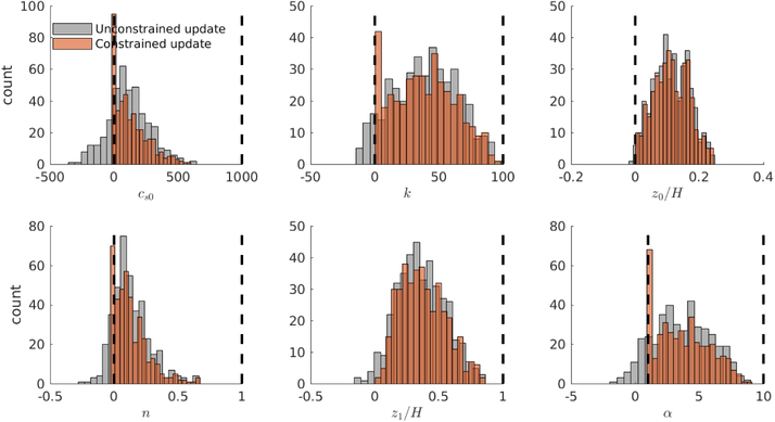
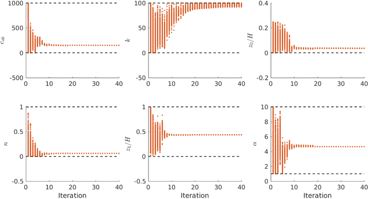
All results shown use Algorithm 7. Figure 4 shows the ensemble distribution of u at J = 2 before and after enforcing constraints whilst Figure 5 shows the evolution of the updated ensemble. Note that parameter k saturates with an ensemble close to the upper bound of 100 imposed through constraints on this parameter; however experiments in which we imposed different upper bounds on this parameter lead to different estimates for k, with little change to the estimated velocity profile and we conclude that this parameter suffers from identifiability issues. (Note that Figure 4 displays the updated ensemble distribution at a single step in the sequence of ensemble updates, comparing the effect of imposing constraints with neglecting them; in contrast Figure 1 shows the distribution over all measurement time-points of the ensemble means. The figures thus illustrate different phenomena).

Figure 4.

The distribution of parameters before and after enforcing constraints in Algorithm 7 at iteration J = 2. Black vertical lines denote the lower and upper bound constraints.

Figure 5.

Evolution of the updated ensemble with iteration. Black horizontal lines denote the lower and upper bound constraints.

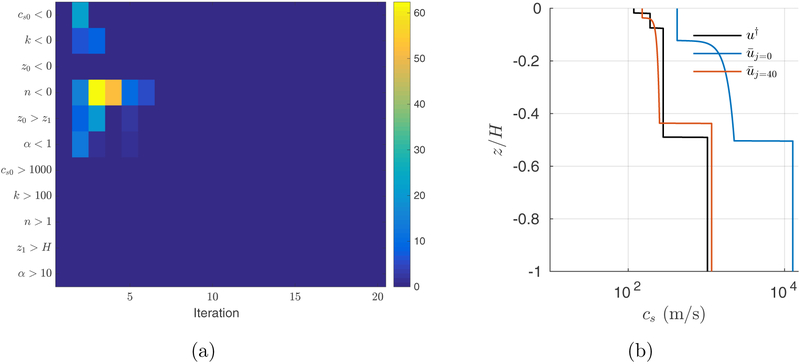
Moreover, Figure 6a shows the map of violation for different constraints enforced on parameters whilst Figure 6b shows the estimated generic c_s profile after 40 iterations compared to the true profile and the initial estimate. Figure 6a shows the key role employed by the enforcing of constraints. In this case the addition of constraints ensures that all the simulations which constitute the ensemble method are physically meaningful, and also that the forward model remains well-posed.

Figure 6.

(a) The percentage map of the constraint violations for the first 20 iterations; (b) the estimated velocity profile $\left({\overline{u}}_{j=40}\right)$ compared to the true profile (u ^†) and the initial estimate $\left({\overline{u}}_{j=0}\right)$

5. Conclusions

Constraints arise naturally in many state and parameter estimation problems. We have shown how convex constraints may be incorporated into ensemble Kalman based state or parameter estimation algorithms with relatively few changes to existing code: the standard algorithm is applied and for any ensemble member which violates a constraint, a quadratic optimization problem subject to convex constraints is solved instead. We have written the resulting algorithms in easily digested pseudo-code, we have developed an underpinning theory and we have given illustrative numerical examples.

Two primary directions suggest themselves in this area. The first is the use of these methods in applications. As indicated in the introduction, our general formulation is inspired by the two papers [8, 6] from the geosciences and we have demonstrated applicability to problems from biomedicine and seismology; but many other potential application domains are ripe for application of ensemble Kalman methodology, because of its black-box and derivative-free formulation, and the ability to impose constraints in a straightforward fashion will help to extend this methodology. The second is the theoretical analysis of these methods: can the inclusion of constraints be used to deduce improved accuracy of state or parameter estimates; or can the inclusion of constraints be used to demonstrate improved performance as measured, for example, by proportion of model runs which are physically (or biologically etc.) plausible? Furthermore, although the imposition of constraints is reasonable, it is not clear that it may not lead to pathologies in algorithmic performance and ruling out, or understanding, the occurrence of such pathological behaviour may be important.

Appendix

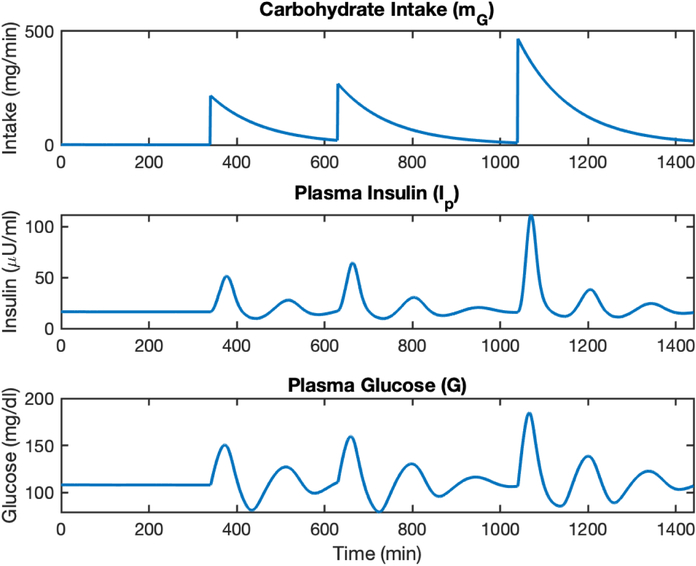
We give the details of the ultradian model of glucose-insulin dynamics used as the forward model in subsection 4.1. An example of the induced dynamics is given in Figure 7.

$$\frac{d{I}_p}{dt}=f_1(G)-E\left(\frac{I_p}{V_p}-\frac{I_i}{V_i}\right)-\frac{I_p}{t_p}$$ (34)

$$\frac{d{I}_i}{dt}=E\left(\frac{I_p}{V_p}-\frac{I_i}{V_i}\right)-\frac{I_i}{t_i}$$ (35)

$$\frac{dG}{dt}=f_4\left(h_3\right)+m_G(t)-f_2(G)-f_3\left(I_i\right)G$$ (36)

$$\frac{d{h}_1}{dt}=\frac{1}{t_d}\left(I_p-h_1\right)$$ (37)

$$\frac{d{h}_2}{dt}=\frac{1}{t_d}\left(h_1-h_2\right)$$ (38)

$$\frac{d{h}_3}{dt}=\frac{1}{t_d}\left(h_2-h_3\right)$$ (39)

where, for N meals at times ${\left\{t_j\right\}}_{j=1}^N$ with carbohydrate composition ${\left\{m_j\right\}}_{j=1}^N$

$$m_G(t)=\sum _{j=1}^N\frac{m_{j}k}{60}\text{exp}\left(k\left(t_j-t\right)\right),N=\#\left\{t_j<t\right\}$$ (40)

and

$$f_1(G)=\frac{R_m}{1+\text{exp}\left(\frac{-G}{V_g{c}_1}+a_1\right)}:\text{ the rate of insulin production}$$ (41)

$$f_2(G)=U_b\left(1-\text{exp}\left(\frac{-G}{C_2{V}_g}\right)\right):\text{insulin-independent glucose utilization}$$ (42)

$$f_3\left(I_i\right)=\frac{1}{C_3{V}_g}\left(U_0+\frac{U_m-U_0}{1+{\left(\kappa I_i\right)}^{-\beta }}\right),f_3\left(I_i\right)G:\text{insulin-dependent glucose utilization}$$ (43)

$$f_4\left(h_3\right)=\frac{R_g}{1+\text{exp}\left(\alpha \left(\frac{h_3}{C_5{V}_p}-1\right)\right)}:\text{delayed insulin-dependent glucose utilization}$$ (44)

$$\kappa =\frac{1}{C_4}\left(\frac{1}{V_i}-\frac{1}{E{t}_i}\right)$$ (45)

Figure 7.

Here we show the oscillating dynamics of the glucose-insulin response in the ultradian model, driven by an exponentially decaying nutritional driver m_G

References

- [1].Teixeira BO, Tôrres LA, Aguirre LA and Bernstein DS 2010. Journal of Process Control 20 45–57 [Google Scholar]
- [2].Bonnet V, Dumas R, Cappozzo A, Joukov V, Daune G, Kulić D, Fraisse P, Andary S and Venture G 2017. Journal of biomechanics 62 140–147 [DOI] [PubMed] [Google Scholar]
- [3].Goffaux G, Perrier M and Cloutier M 2011. Cell energy metabolism: a constrained ensemble kalman filter Proceedings of the 18th IFAC world congress: Milano, Italy, International Federation of Automatic Control; pp 8391–8396 [Google Scholar]
- [4].Lei J, Liu S and Wang X 2012. IET Science, Measurement & Technology 6 63–77 [Google Scholar]
- [5].Simon D and Simon DL 2010. International Journal of Systems Science 41 159–171 [Google Scholar]
- [6].Janjić T, McLaughlin D, Cohn SE and Verlaan M 2014. Monthly Weather Review 142 755–773 [Google Scholar]
- [7].Yang X, Huang B and Prasad V 2014. Chemical Engineering Science 106 211–221 [Google Scholar]
- [8].Wang D, Chen Y and Cai X 2009. Water resources research 45 [Google Scholar]
- [9].Aravkin AY, Burke JV and Pillonetto G 2014. Optimization viewpoint on kalman smoothing with applications to robust and sparse estimation Compressed Sensing & Sparse Filtering (Springer; ) pp 237–280 [Google Scholar]
- [10].Aravkin A, Burke JV, Ljung L, Lozano A and Pillonetto G 2017. Automatica 86 63–86 [Google Scholar]
- [11].Evensen G 2009. Data assimilation: the ensemble Kalman filter (Springer Science & Business Media; ) [Google Scholar]
- [12].Reich S and Cotter C 2015. Probabilistic forecasting and Bayesian data assimilation (Cambridge University Press; ) [Google Scholar]
- [13].Law K, Stuart A and Zygalakis K 2015. Data Assimilation (Springer; ) [Google Scholar]
- [14].Carrassi A, Bocquet M, Bertino L and Evensen G 2018. Data assimilation in the geosciences: An overview of methods, issues, and perspectives vol 9 (Wiley Interdisciplinary Reviews: Climate Change, 5(2018)) [Google Scholar]
- [15].Evensen G 1994. Journal of Geophysical Research: Oceans 99 10143–10162 [Google Scholar]
- [16].Burgers G, Jan van Leeuwen P and Evensen G 1998. Monthly weather review 126 1719–1724 [Google Scholar]
- [17].Oliver DS, Reynolds AC and Liu N 2008. Inverse theory for petroleum reservoir characterization and history matching (Cambridge University Press; ) [Google Scholar]
- [18].Iglesias MA, Law KJ and Stuart AM 2013. Inverse Problems 29 045001 [Google Scholar]
- [19].Doucet A, De Freitas N and Gordon N 2001. An introduction to sequential monte carlo methods Sequential Monte Carlo methods in practice (Springer; ) pp 3–14 [Google Scholar]
- [20].Del Moral P, Doucet A and Jasra A 2006. Journal of the Royal Statistical Society: Series B (Statistical Methodology) 68 411–436 [Google Scholar]
- [21].Simon D 2010. IET Control Theory & Applications 4 1303–1318 [Google Scholar]
- [22].Amor N, Rasool G and Bouaynaya NC 2018. Constrained state estimation — a review (Preprint arXiv:1807.03463)
- [23].Robertson DG, Lee JH and Rawlings JB 1996. AIChE Journal 42 2209–2224 [Google Scholar]
- [24].Rao CV, Rawlings JB and Mayne DQ 2003. IEEE transactions on automatic control 48 246–258 [Google Scholar]
- [25].Vachhani P, Rengaswamy R, Gangwal V and Narasimhan S 2005. AIChE Journal 51 946–959 [Google Scholar]
- [26].Li R, Jan NM, Prasad V and Huang B 2018. Constrained extended kalman filter based on kullback-leibler (kl) divergence 2018 European Control Conference (ECC) (IEEE; ) pp 831–836 [Google Scholar]
- [27].Vachhani P, Narasimhan S and Rengaswamy R 2006. Journal of process control 16 1075–1086 [Google Scholar]
- [28].Julier S, Uhlmann J and Durrant-Whyte HF 2000. IEEE Transactions on automatic control 45 477–482 [Google Scholar]
- [29].Simon D and Simon DL 2006. IEE Proceedings-Control Theory and Applications 153 371–378 [Google Scholar]
- [30].Mandela R, Kuppuraj V, Rengaswamy R and Narasimhan S 2012. Journal of Process Control 22 718–728 [Google Scholar]
- [31].Prakash J, Patwardhan SC and Shah SL 2008. 2008 American Control Conference 3542–3547 [Google Scholar]
- [32].Prakash J, Patwardhan SC and Shah SL 2010. Industrial & Engineering Chemistry Research 49 2242–2253 [Google Scholar]
- [33].Stuart A and Zygalakis K 2015. Data assimilation: A mathematical introduction Tech. rep Oak Ridge National Laboratory (ORNL), Oak Ridge, TN (United States) [Google Scholar]
- [34].Albers DJ, Levine M, Gluckman B, Ginsberg H, Hripcsak G and Mamykina L 2017. PLoS computational biology 13 e1005232. [DOI] [PMC free article] [PubMed] [Google Scholar]
- [35].Sturis J, Polonsky KS, Mosekilde E and Van Cauter E 1991. American Journal of Physiology-Endocrinology And Metabolism 260 E801–E809 [DOI] [PubMed] [Google Scholar]
- [36].Shi J and Asimaki D 2018. Seismological Research Letters 89 1397–1409 [Google Scholar]