Intelligent computing with Levenberg–Marquardt artificial neural networks for nonlinear system of COVID-19 epidemic model for future generation disease control

Abstract

The aim of this work is to design an intelligent computing paradigm through Levenberg–Marquardt artificial neural networks (LMANNs) for solving the mathematical model of Corona virus disease 19 (COVID-19) propagation via human to human interaction. The model is represented with systems of nonlinear ordinary differential equations represented with susceptible, exposed, symptomatic and infectious, super spreaders, infection but asymptomatic, hospitalized, recovery and fatality classes, and reference dataset of the COVID-19 model is generated by exploiting the strength of explicit Runge–Kutta numerical method for metropolitans of China and Pakistan including Wuhan, Karachi, Lahore, Rawalpindi and Faisalabad. The created dataset is arbitrary used for training, validation and testing processes for each cyclic update in Levenberg–Marquardt backpropagation for numerical treatment of the dynamics of COVID-19 model. The effectiveness and reliable performance of the design LMANNs are endorsed on the basis of assessments of achieved accuracy in terms of mean squared error based merit functions, error histograms and regression studies.

Introduction

In December 2019, a new disease known as coronavirus was declared as a viral infection with high rate of transmission in Wuhan city of China. Corona virus (COVID-19) is originated by the acute respiratory syndrome 2 (SARS-Covid-2) declared by the Group of International Committee (GIC) on Taxonomy of virus on February 11, 2020. It was identified as the causative virus by Chinese authorities on January 1, 2020 [1]. A chain of analysis reported on Bats are key reservoir in this research [2, 3].

An overview of COVID-19 epidemic

The COVID-19 epidemic mainly effects on people’s health, economy daily life routine [4]. Due to these major causes, the governments of several countries have made public policy about both highlighted aspects. The 2019 crown infection likewise called the Wuhan crown infection, is a transmitted infection causing respiratory disease and exceptionally transmitted from human to human. The Covide-19 epidemic is considered highest threat for the whole world due to thousands of people are infected. It was noticed that on March 26, 2020, total infected confirmed cases are 503,274 with 22,342 number of deaths. Later, the number of infected cases reached to 1,353,361 with 79,235, total number of deaths, reported on April 8, 2020, by the World Health Organization (WHO). The present statistics of confirm cases are 17,918,582, with newly reported in last 24 h are 257,677 for COVID-19, while cumulative deaths are 686,703 and newly reported deaths in last 24 h are 5810 on August 03, 2020 by WHO.

The story of coronavirus (COVID-19) originally started on December 31, 2019, from Wuhan city of China, which is now the capital of Hubei territory. In the previous medical history of viruses, spreading of viruses always have some logical reasoning for which the accessible medications are found for the treatment. Further, it has been verified through reliable data that the transmission of the infection is only possible from humans to humans [5]. During the reported time, many cases were spread in Wuhan city as well as to different urban communities of China rapidly. Besides this, the infection spreads to other parts of the world, for example, Europe, North America and Asia within short span of time. Meanwhile it is reported that the appearance of the symptoms based on cough, breathing troubles and high fever of the corona (COVID-19) within 2 to 10 or 2 to 14 days approximately.

Related studies

Nowadays, the dynamics of COVID-19 models have been growing interest in the research community and may mathematical models are designed for the better interest of people around the world, such as the model of eight classes based on susceptible, infected, diagnosed, ailing, recognized, threatened, healed and extinct (SIDARTHE) [6], five classes based on SEIAR represented with 5 number of ordinary differential equations [7], a new θ-SEIHRD model represented with nine classes [8], modified SEIRS model system with five classes [9], four class modified SIR model [10], SAIR system based COVID-19 model for complex networks [11]. Beside, these variety of COVID-19 model are introduced by the researchers [8, 12–22]. However, in the current scenarios, we have taken a complex 8 classes model based on Susceptible (S), exposed (E), symptomatic and infectious (I), super propagation (P), infection but asymptomatic (A), hospitalized (H), recovery (R) and fatality (F) classes, i.e., SEIPAHRF for numerical investigations [23].

System model

Mathematical relations of Covid-19 dynamics with SEIPAHRF model are represented with following initial value problem (IVP) as [23]:

$$\begin{array}{cc}\hfill \frac{\text{d}S}{\text{d}t}& =-(\beta /N)I(t)S(t)-(l\beta /N)H(t)S(t)\hfill \\ \hfill & -({\beta }_1/N)P(t)S(t)\hfill \\ \hfill \end{array}$$ 1

$$\begin{array}{cc}\hfill \frac{\text{d}E}{\text{d}t}& =(\beta /N)I(t)S(t)+(l\beta /N)H(t)S(t)\hfill \\ \hfill & +({\beta }_1/N)P(t)S(t)-kE(t)\hfill \\ \hfill \end{array}$$ 2

$$\frac{\text{d}I}{\text{d}t}=k{\rho }_{1}E(t)-({\gamma }_a+{\gamma }_i)I(t)-{\delta }_{i}I(t)$$ 3

$$\frac{\text{d}P}{\text{d}t}=k{\rho }_{2}E(t)-({\gamma }_a+{\gamma }_i)P(t)-{\delta }_{p}P(t)$$ 4

$$\frac{\text{d}A}{\text{d}t}=k(1-{\rho }_1-{\rho }_2)E(t)$$ 5

$$\frac{\text{d}H}{\text{d}t}={\gamma }_a(I(t)+P(t))-{\gamma }_{r}H(t)-{\delta }_{h}H(t)$$ 6

$$\frac{\text{d}R}{\text{d}t}={\gamma }_i(I(t)+P(t))+{\gamma }_{r}H(t)$$ 7

$$\frac{\mathit{dF}}{\mathit{dt}}={\delta }_{i}I(t)+{\delta }_{p}P(t)+{\delta }_{h}H(t)$$ 8

$$\begin{array}{cc}\hfill S(0)& =N-6,E(0)=0,I(0)=1,P(0)=5,\hfill \\ \hfill A(0)& =0,H(0)=0,R(0)=0,F(0)=0\hfill \\ \hfill \end{array}$$ 9

where definitions of each parameter of COVID-19 on SEIPAHRF model (1–9) is provided in nomenclature table. The graphical representation of SEIPAHRF model for COVID-19 dynamics is shown in Fig. 1 to decipher the information more evidently.

Fig. 1.

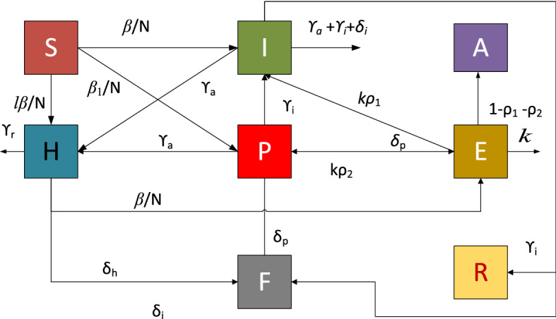
Eight classes based SEIPAHRF model of COVID-19 dynamics

Problem statement with significance

The strength of artificial intelligent (AI) based computing solvers has been exploited by the research community on large scale to obtain the approximated solutions of many problems arises in broad fields of applied science and technology. Some potential, recent reported studies having paramount significance including Van-der-Pol oscillatory systems, optics, electrically conducting solids, reactive transport system, nanofluidics, nanotechnology, fluid dynamics, astrophysics, circuit theory, plasma, atomic physics, bioinformatics, energy, power and functional mathematics see [24–34] and references cited therein. The said information is the motivational affinities to investigate in AI base numerical computing solver for the COVID-19 model.

As per our literature survey no one yet implemented AI based computational procedure through Levenberg–Marquardt artificial neural networks (LMANNs) to solve initial value problems (IVBs) of nonlinear systems of ordinary differential equations (ODEs) represented COVID dynamics as given in (1–9). We present the design of intelligent computing paradigm through LMANNs for numerical treatment of Covid-19 based SEIPAHRF model for five different cities of China and Pakistan including Wuhan, Karachi, Lahore, Rawalpindi and Faisalabad. Research related Covid-19 model and its applications will be useful to different models of diseases emerging in science, particularly, bio-mathematicians for design and development of alternate computing solver to study the dynamics of the systems numerically.

Innovative contributions

The innovative contributions of the presented study for Levenberg–Marquardt artificial neural networks (LMANNs) for COVID-19 models are highlighted as follows.

• A novel design based on two-layers structure of Levenberg–Marquardt artificial neural networks (LMANNs) is presented to examine the dynamics of COVID-19 model represented with initial value problems of eight systems of ODEs.

• The mean squared error (MSE) index is used effectively to develop a merit function for analysis of computational results of designed LMANNs by taking reference solutions of eight classes based model of SEIPAHRF for COVID-19 pandemic with the help of implicit Runge–Kutta methods.

• Levenberg–Marquardt backpropagation is exploited for conducting training, validation and testing processes to tune the decision variables of ANNs for each increment of epoch index.

• Reliability, convergence and accurate performance of LMANNs to solve the COVID-19 models with dataset for five cities including Wuhan, Karachi, Lahore, Faisalabad and Rawalpindi is endorsed through histograms with error analysis, correlation and regression curves.

Organization

The mathematical models for the development for the COVID-19 systems for one big city of China and 4 cities of Pakistan are presented in Sect. 2, methodology of LMANNs is provided in Sect. 3, the numerical simulation and analysis are presented for different cases COVID-19 dynamics in Sect. 4, while concluding inferences are given in the last Section.

Mathematical formulation of COVID-19 models

Mathematical development of COVID-19 for different cities of China and Pakistan is provided in this section. Fixed setting of parameters as tabulated in Table 1 reported recently in [23] for SEIPAHRF model of COVID-19 is used throughout in the presented study.

Table 1.

Parameter setting for SEIPAHRF model of COVID-19 dynamics

Parameter	Value	Units
β	2.55	day−1
β1	7.65	day−1
k	0.25	day−1
ρ1	0.580	Dimensionless
ρ2	0.001	Dimensionless
γa	0.94	day−1
γi	0.27	day−1
γr	0.5	day−1
δi	3.5	day−1
δp	1	day−1
δh	0.3	day−1
l	1.56	Dimensionless

COVID-19 model for Wuhan, China

Consider a dynamical system of equations representing Covid-19 model of Wuhan City of China written as

$$\begin{array}{cc}\hfill \frac{\text{d}S}{\text{d}t}& =-5.79545\times {10}^{-5}I(t)S(t)-8.98295\times {10}^{-5}H(t)S(t)\hfill \\ \hfill & -1.7386\times {10}^{-4}P(t)S(t)\hfill \\ \hfill \frac{\text{d}E}{\text{d}t}& =5.79545\times {10}^{-5}I(t)S(t)+8.98295\times {10}^{-5}H(t)S(t)\hfill \\ \hfill & +1.7386\times {10}^{-4}P(t)S(t)-0.25E(t)\hfill \\ \hfill \frac{\text{d}I}{\text{d}t}& =0.145E(t)-1.21I(t)-3.5I(t)\hfill \\ \hfill \frac{\text{d}P}{\text{d}t}& =2.5\times {10}^{-4}E(t)-2.21P(t)\hfill \\ \hfill \frac{\text{d}A}{\text{d}t}& =0.1047E(t)\hfill \\ \hfill \frac{\text{d}H}{\text{d}t}& =0.94(I(t)+P(t))-H(t)-0.3H(t)\hfill \\ \hfill \frac{\text{d}R}{\text{d}t}& =3.5(I(t)+P(t))+H(t)\hfill \\ \hfill \frac{\text{d}F}{\text{d}t}& =3.5I(t)+P(t)+0.3H(t)\hfill \\ \hfill S(0)& =43994,E(0)=0,I(0)=1,P(0)=5,\hfill \\ \hfill A(0)& =0,H(0)=0,R(0)=0,F(0)=0\hfill \\ \hfill \end{array}$$ 10

COVID-19 model for Karachi, Pakistan

Consider a dynamical system of equations representing Covid-19 model of Karachi City of Pakistan written as

$$\begin{array}{cc}\hfill \frac{\text{d}S}{\text{d}t}& =-6.826212\times {10}^{-5}I(t)S(t)-1.0648\times {10}^{-4}H(t)S(t)\hfill \\ \hfill & -2.0478\times {10}^{-4}P(t)S(t)\hfill \\ \hfill \frac{\text{d}E}{\text{d}t}& =6.826212\times {10}^{-5}I(t)S(t)+1.0648\times {10}^{-4}H(t)S(t)\hfill \\ \hfill & +2.0478\times {10}^{-4}P(t)S(t)-0.25E(t)\hfill \\ \hfill \frac{\text{d}I}{\text{d}t}& =0.145E(t)-1.21I(t)-3.5I(t)\hfill \\ \hfill \frac{\text{d}P}{\text{d}t}& =2.5\times {10}^{-4}E(t)-2.21P(t)\hfill \\ \hfill \frac{\text{d}A}{\text{d}t}& =0.1047E(t)\hfill \\ \hfill \frac{\text{d}H}{\text{d}t}& =0.94(I(t)+P(t))-H(t)-0.3H(t)\hfill \\ \hfill \frac{\text{d}R}{\text{d}t}& =3.5(I(t)+P(t))+H(t)\hfill \\ \hfill \frac{\text{d}F}{\text{d}t}& =3.5I(t)+P(t)+0.3H(t)\hfill \\ \hfill S(0)& =37350,E(0)=0,I(0)=1,P(0)=5,\hfill \\ \hfill A(0)& =0,H(0)=0,R(0)=0,F(0)=0\hfill \\ \hfill \end{array}$$ 11

COVID-19 model for Lahore, Pakistan

Consider a dynamical system of equations representing Covid-19 model of Lahore City of Pakistan written as

$$\begin{array}{cc}\hfill \frac{\text{d}S}{\text{d}t}& =-1.2394\times {10}^{-4}I(t)S(t)-1.9336\times {10}^{-4}H(t)S(t)\hfill \\ \hfill & -3.7184\times {10}^{-4}P(t)S(t)\hfill \\ \hfill \frac{\text{d}E}{\text{d}t}& =1.2394\times {10}^{-4}I(t)S(t)+1.9336\times {10}^{-4}H(t)S(t)\hfill \\ \hfill & +3.7184\times {10}^{-4}P(t)S(t)-0.25E(t)\hfill \\ \hfill \frac{\text{d}I}{\text{d}t}& =0.145E(t)-1.21I(t)-3.5I(t)\hfill \\ \hfill \frac{\text{d}P}{\text{d}t}& =2.5\times {10}^{-4}E(t)-2.21P(t)\hfill \\ \hfill \frac{\text{d}A}{\text{d}t}& =0.1047E(t)\hfill \\ \hfill \frac{\text{d}H}{\text{d}t}& =0.94(I(t)+P(t))-H(t)-0.3H(t)\hfill \\ \hfill \frac{\text{d}R}{\text{d}t}& =3.5(I(t)+P(t))+H(t)\hfill \\ \hfill \frac{\text{d}F}{\text{d}t}& =3.5I(t)+P(t)+0.3H(t)\hfill \\ \hfill S(0)& =20567,E(0)=0,I(0)=1,P(0)=5,\hfill \\ \hfill A(0)& =0,H(0)=0,R(0)=0,F(0)=0\hfill \\ \hfill \end{array}$$ 12

COVID-19 model for Faisalabad, Pakistan

Consider a dynamical system of equations representing Covid-19 model of Faisalabad City of Pakistan written as

$$\begin{array}{cc}\hfill \frac{\text{d}S}{\text{d}t}& =-3.1736\times {10}^{-4}I(t)S(t)-4.9508\times {10}^{-4}H(t)S(t)\hfill \\ \hfill & -9.5208\times {10}^{-4}P(t)S(t)\hfill \\ \hfill \frac{\text{d}E}{\text{d}t}& =3.1736\times {10}^{-4}I(t)S(t)+4.9508\times {10}^{-4}H(t)S(t)\hfill \\ \hfill & +9.5208\times {10}^{-4}P(t)S(t)-0.25E(t)\hfill \\ \hfill \frac{\text{d}I}{\text{d}t}& =0.145E(t)-1.21I(t)-3.5I(t)\hfill \\ \hfill \frac{\text{d}P}{\text{d}t}& =2.5\times {10}^{-4}E(t)-2.21P(t)\hfill \\ \hfill \frac{\text{d}A}{\text{d}t}& =0.1047E(t)\hfill \\ \hfill \frac{\text{d}H}{\text{d}t}& =0.94(I(t)+P(t))-H(t)-0.3H(t)\hfill \\ \hfill \frac{\text{d}R}{\text{d}t}& =3.5(I(t)+P(t))+H(t)\hfill \\ \hfill \frac{\text{d}F}{\text{d}t}& =3.5I(t)+P(t)+0.3H(t)\hfill \\ \hfill S(0)& =43994,E(0)=0,I(0)=1,P(0)=5,\hfill \\ \hfill A(0)& =0,H(0)=0,R(0)=0,F(0)=0\hfill \\ \hfill \end{array}$$ 13

COVID-19 model for Rawalpindi, Pakistan

Consider a dynamical system of equations representing Covid-19 model of Rawalpindi City of Pakistan written as

$$\begin{array}{cc}\hfill \frac{\text{d}S}{\text{d}t}& =-4.5220\times {10}^{-4}I(t)S(t)-7.0544\times {10}^{-4}H(t)S(t)\hfill \\ \hfill & -1.35662\times {10}^{-3}P(t)S(t)\hfill \\ \hfill \frac{\text{d}E}{\text{d}t}& =4.5220\times {10}^{-4}I(t)S(t)+7.0544\times {10}^{-4}HH(t)S(t)\hfill \\ \hfill & +1.35662\times {10}^{-3}P(t)S(t)-0.25E(t)\hfill \\ \hfill \frac{\text{d}I}{\text{d}t}& =0.145E(t)-1.21I(t)-3.5I(t)\hfill \\ \hfill \frac{\text{d}P}{\text{d}t}& =2.5\times {10}^{-4}E(t)-2.21P(t)\hfill \\ \hfill \frac{\text{d}A}{\text{d}t}& =0.1047E(t)\hfill \\ \hfill \frac{\text{d}H}{\text{d}t}& =0.94(I(t)+P(t))-H(t)-0.3H(t)\hfill \\ \hfill \frac{\text{d}R}{\text{d}t}& =3.5(I(t)+P(t))+H(t)\hfill \\ \hfill \frac{\text{d}F}{\text{d}t}& =3.5I(t)+P(t)+0.3H(t)\hfill \\ \hfill S(0)& =5633,E(0)=0,I(0)=1,P(0)=5,\hfill \\ \hfill A(0)& =0,H(0)=0,R(0)=0,F(0)=0\hfill \\ \hfill \end{array}$$ 14

Methodology and performance metrics

The essential information related to our proposed mathematical modeling together with performance metrics are presented in this section.

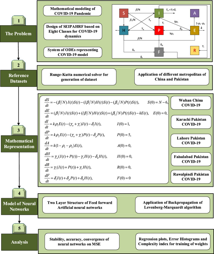
The implemented mathematical modeling based on three phases: in phase one COVID-19 model for five different cities of China-Pakistan is evaluated that are considered as input reference dataset for FFNNs, phase two, layer structure formulation of NN-BPML models and training of NN-BPML is performed with Levenberg-Marquart solver in phase three. The graphical abstract of presented study is shown in Fig. 2.

Fig. 2.

Process flow architecture of Proposed Methodology NN-BPML for solving COVID-19 model

The Adams predictor corrector method procedure [60–61] is presented to the system (9–10). By using Adams method formulation, first we used predictor solution then corrected in whole numerical procedure to improve the accuracy level of results with provided information of predicted results. The Eqs. (9–10) of predictor corrector method can be given as:

$$\begin{array}{cc}\hfill \frac{\text{d}S}{\text{d}t}& =f(t,S,I,H,P),S(t_0)=S_0\hfill \\ \hfill \frac{\text{d}E}{\text{d}t}& =f(t,E,I,S,H,P),E(t_0)=E_0\hfill \\ \hfill \frac{\text{d}I}{\text{d}t}& =f(t,I,E),I(t_0)=I_0\hfill \\ \hfill \frac{\text{d}P}{\text{d}t}& =f(t,P,E),P(t_0)=P_0\hfill \\ \hfill \frac{\text{d}A}{\text{d}t}& =f(t,E),A(t_0)=A_0\hfill \\ \hfill \frac{\text{d}H}{\text{d}t}& =f(t,H,I,P),H(t_0)=H_0\hfill \\ \hfill \frac{\text{d}R}{\text{d}t}& =f(t,I,P,H),R(t_0)=R_0\hfill \\ \hfill \frac{\text{d}F}{\text{d}t}& =f(t,I,P,H),F(t_0)=F_0\hfill \\ \hfill \end{array}$$ 15

The relation for predictor 2-step formula in case of first equation of set (15) is given:

$$S_{n+1}=S_n+1.5hf(t_n,S_n)-0.5hf(t_{n-1},S_{n-1}),$$ 16

while 2-step corrector relation formula in case of first equation of set (15) is written as:

$$S_{n+1}=S_n+0.5h(f(t_{n+1},S_{n+1})+f(t_n,S_n))$$ 17

Accordingly, the formulae of Adam predictor and corrector method for rest of equations in set (15) are formulated. The dataset of FFNN can be created with Adams method as summarized in Eqs. (11–13) for solving the PLFMs. However, the presented study, we have generated the dataset of FFNN using ‘NDSolve’ routine of Mathematica with algorithm ‘Adams’ for each scenario of PLFMs.

The layer structure of FFNN models with log-sigmoid activation function and 10 number of neurons in the hidden layer are exploited for solving each scenario of PLFMs. The constructed architecture of FFNN is presented in Fig. 3

Fig. 3.

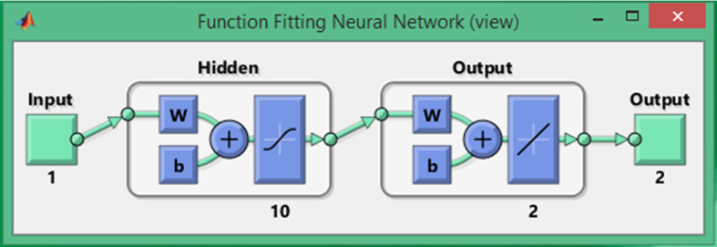
FFNN architecture in terms of input, hidden and output layers

The training the FFNNs is conducted with backpropagation of Levenberg-Marquardt method (LMM), i.e., FFNN-LMM by defining an error base merit function. The objective function is constructed of mean square error (MSE) metric and optimization of the objective function is performed with LMM for each case.

The mathematical notations of the performance metrics through absolute error (AE), figure of merit, i.e., mean square error (MSE) and regression coefficient are given below:

$$\begin{array}{cc}\hfill \text{AE}& =\left|S_j-{\widehat{S}}_j\right|,j=1,2,\dots ,k,\hfill \\ \hfill \text{MSE}& =\frac{1}{k}\sum _{j=1}^k{\left(S_j-{\widehat{S}}_j\right)}^2,\hfill \\ \hfill R^2& =1-\frac{{\sum }_{j=1}^k{\left({\widehat{S}}_j-{\overline{S}}_j\right)}^2}{{\sum }_{j=1}^k{\left(S_j-{\overline{S}}_j\right)}^2}\hfill \\ \hfill \end{array}$$ 18

here S_j, ${\widehat{S}}_j$ and ${\overline{S}}_j$ stand for reference, approximate and mean of solution of jth input, while k represent total number of input grids. The unit value of R, i.e., square root of R², is the desire parameter for perfect modeling, while AE and MSE are equal to zero for perfect modeling scenarios.

Numerical simulation with interpretations

Numerical simulations studies along with necessary interpretation are presented here for system of first order nonlinear ODEs (1–9) representing the epidemic model of SEIPAHRF system for COVID-19 with the help of the proposed LMANNs method. The numerical along with the graphical results of five different metropolitans of China and Pakistan included Wuhan, Karachi, Lahore, Faisalabad and Rawalpindi are presented using set of Eqs. (10–14).

The overall process flow diagram of proposed LMANNs is described in Fig. 2. The proposed LMANNs are implemented through ‘nftool’ (neural network fitting tool) in neural network toolbox in Matlab environment, while Levenberg–Marquardt (L–M) is used to train the weights of neural networks. The designed LMANNs are conducted for five different cases where first four cases are constructed on real data of big cities of Pakistan: Karachi, Lahore, Faisalabad and Rawalpindi, and last case is on real data of Wuhan city with fixed parameters as tabulated in Table 1. The papulation survey of 2017 of Pakistan is used for related parameters.

The reference data of SEIPAHRF model for COVID-19 are generated for 60 days as inputs with step size of 0.5 through the solutions of Adams numerical approach by using Mathematica environment ‘NDSolve’ built-in function for numerical results of ODEs for each case of SEIPAHRF model for COVID-19. The dataset values for S, E, I, P, A, H, R and F classes for 121 input points that are arbitrarily distributed to produce a set for train, validation and test with 90%, 5% and 5%, respectively. The two layered structure LMANNs based computing paradigm of neural networks with backpropagation of L–M along ten hidden layers are contracted for the results of SEIPAHRF mode for COVID-19 classes that shown in Fig. 3.

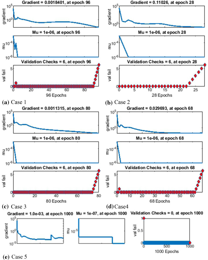
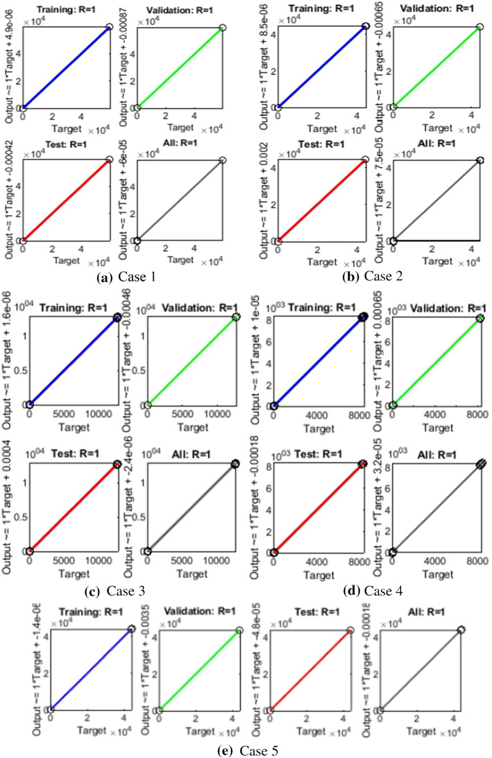
The results of LMANNs for SEIPAHRF model for COVID-19 in terms of state transition dynamics are graphically described in Fig. 4, while fitting of solution along with the performance and error histograms are illustrated in Figs. 5, 6, 7, 8 and 9 for case 1–5, the regression analysis are shown in Fig. 10 for each case. Moreover, the convergence achieved parameter in terms of MSE, back propagation measures, performance, executed epochs and time of execution are tabulated in Tables 2, for all cases of SEIPAHRF model for COVID-19 through LMANNs, and the mentioned time of all cases explains the complexity of the proposed method.

Fig. 4.

State transition dynamics of NN-BPML for solving the COVID-19 mode for case 1-5

Fig. 5.

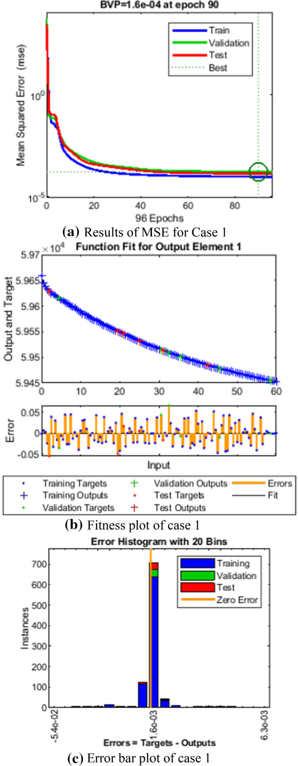
Comparison of LMANNs results with reference solution, performance analysis and error histogram for case 1

Fig. 6.

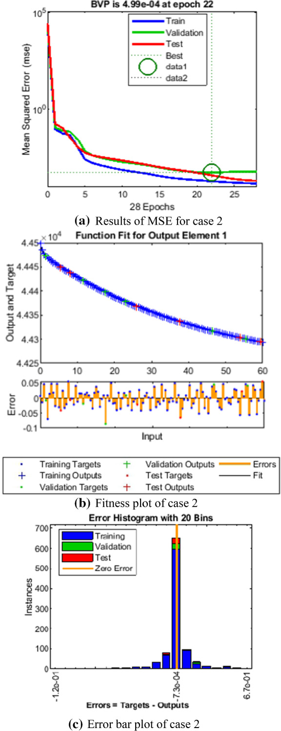
Comparison of LMANNs results with reference solution, performance analysis and error histogram for case 2

Fig. 7.

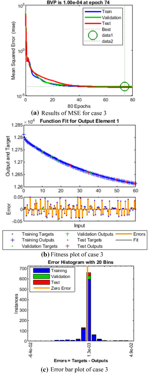
Comparison of LMANNs results with reference solution, performance analysis and error histogram for case 3

Fig. 8.

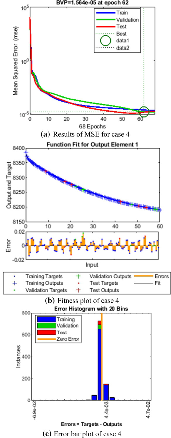
Comparison of LMANNs results with reference solution, performance analysis and error histogram for case 4

Fig. 9.

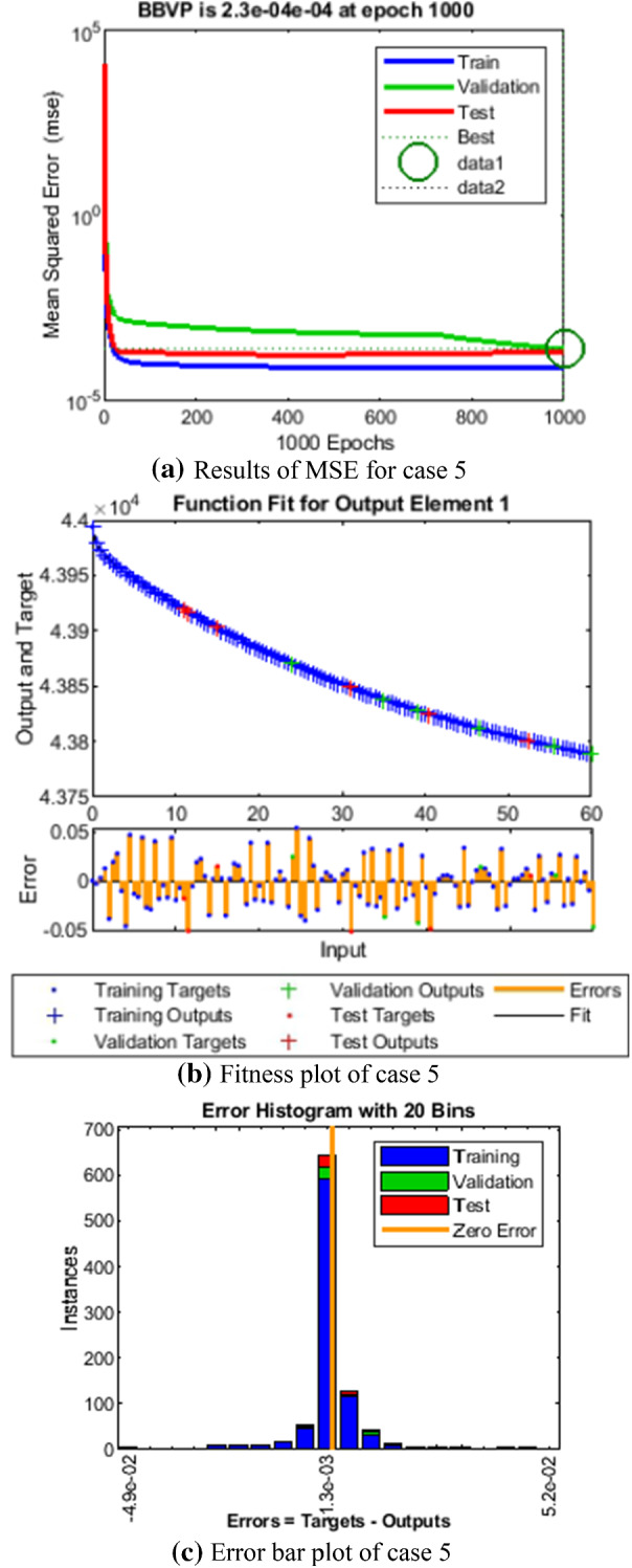
Comparison of LMANNs results with reference solution, performance analysis and error histogram for case 5

Fig. 10.

Regression illustrations for LMANNs result for case 1–5 of SEIPAHRF model for COVID-19

Table 2.

Results of NN-BPLM for each case of COVID-19 model

Case	Mean square error			Performance	Gradient	Mu	Epoch	Time
	Training	Validation	Testing
1	9.7083e−05	1.6596e−0	1.3610e−04	9.64e−05	1.84e−03	1e−06	96	< 0.5
2	1.7914e−04	4.9947e−04	3.5796e−04	1.38e−04	1.10e−01	1e−06	28	< 0.5
3	8.7912e−05	1.0044e−04	8.5482e−05	8.70e−05	1.13e−03	1e−06	80	< 0.5
4	2.3975e−05	1.5640e−05	1.4822e−05	2.14e−05	2.97e−02	1e−06	68	< 0.5
5	7.1286e−05	2.3021e−04	1.8626e−04	7.13e−05	1.01e−03	1e−07	1000	8

The gradient values and step size Mu of backpropagation are about [1.8 × 10⁻⁰³, 1.1 × 10⁻⁰¹, 1.1 × 10⁻⁰³, 2.9 × 10⁻⁰² and 1.0 × 10⁻⁰³] and [10⁻⁰⁶, 10⁻⁰⁶, 10⁻⁰⁶, 10⁻⁰⁶, and 10⁻⁰⁷] as shown in Figs. 4a–e for five cases, respectively. The results determine the accurate and convergent performance of the proposed method for each five cases of SEIPAHRF model for COVID-19.

In the Figs. 5a, 6a, 7a, 8a and 9a, convergence through MSE for validation, train and test processes are illustrated for case 1–5 of SEIPAHRF model for COVID-19. The best network performance achieved at 90, 22, 74, 62 and 1000 epochs with MSE around 10⁻⁰⁴ to 10⁻⁰³, 10⁻⁰⁴ to 10⁻⁰², 10⁻⁰⁴, 10⁻⁰⁵ and 10⁻⁰⁴ to 10⁻⁰³ for case 1–5, respectively. The performance of LMANNs generated outcomes is examined with reference results of Adams numerical method for case 1–5 and respective results are shown in Figs. 5b, 6b, 7b, 8b and 9b that illustrated the curves are overlap each other that means the results are accurate. Along with the error dynamics for input between 0 and 60 with step size of 0.5. The maximum error attained for test, train and validation data by the proposed LMANNs is less than 5 × 10⁻⁰², 5 × 10⁻⁰², 5 × 10⁻⁰², 2 × 10⁻⁰² and 4 × 10⁻⁰⁴ for cases of SEIPAHRF model for COVID-19. These subfigures explain the numerical values of S class where numerical values of other related class are tabulated in Tables 3, 4, 5, 6 and 7 for five cases, respectively. The error dynamics is additional estimated through error histograms for each input point and results are graphically illustrated in Figs. 5c, 6c, 7c, 8c and 9c, respectively, of SEIPAHRF model for COVID-19. The error bin with reference zero line has error around 1.6 × 10⁻⁰³, − 7.3 × 10⁻⁰⁴, 1.3 × 10⁻⁰³, 4.4 × 10⁻⁰³ and 1.3 × 10⁻⁰³ for all five cases, respectively which illustrates more of the results value of the proposed method lies over the zero line.

Table 3.

Numerical values of case 1 against input day for all classes of SEIPAHRF model for COVID-19

Time	Case 1
	S	A	R	F	E	I	P	H
0	59,659.00	− 0.0010	00.0002	00.0055	00.0024	0.9850	5.0009	0.0020
6	59,607.96	12.4825	04.6574	17.1976	21.2499	0.6464	0.0051	0.8044
12	59,580.54	25.0309	07.9092	31.5190	18.7088	0.5772	0.0025	0.7014
18	59,556.49	36.0619	10.7651	44.1122	16.4410	0.5093	0.0017	0.6163
24	59,535.36	45.7526	13.2744	55.1772	14.4426	0.4476	0.0014	0.5414
30	59,516.81	54.2594	15.4774	64.8911	12.6835	0.3926	0.0014	0.4755
36	59,500.53	61.7365	17.4137	73.4291	11.1335	0.3444	0.0013	0.4174
42	59,486.21	68.3021	19.1142	80.9264	09.7694	0.3021	0.0011	0.3663
48	59,473.66	74.0721	20.6086	87.5151	08.5686	0.2650	0.0010	0.3213
54	59,462.55	79.1576	21.9257	93.3222	07.5093	0.2323	0.0009	0.2816
60	59,452.70	83.6890	23.0993	98.4966	06.5656	0.2027	0.0007	0.2463

Table 4.

Numerical values of case 2 against input day for all classes of SEIPAHRF model for COVID-19

Time	Case 2
	S	A	R	F	E	I	P	H
0	44,498.99	− 0.0002	− 0.0009	0.01620	0.01080	0.9461	4.9940	0.0189
6	44,447.97	12.4809	04.6540	17.1999	21.2338	0.6488	− 0.0014	0.8127
12	44,420.59	25.0286	07.9085	31.5179	18.6911	0.5770	0.0015	0.7022
18	44,396.59	36.0317	10.7584	44.0780	16.4207	0.5086	0.0023	0.6146
24	44,375.48	45.7084	13.2642	55.1284	14.4131	0.4461	0.0018	0.5400
30	44,357.00	54.2014	15.4638	64.8270	12.6446	0.3912	0.0015	0.4740
36	44,340.75	61.6583	17.3953	73.3423	11.0869	0.3429	0.0013	0.4158
42	44,326.57	68.1749	19.0833	80.7840	09.7217	0.3007	0.0011	0.3646
48	44,314.13	73.8953	20.5652	87.3165	08.5204	0.2635	0.0010	0.3196
54	44,303.18	78.9241	21.8680	93.0593	07.4621	0.2308	0.0009	0.2799
60	44,293.61	83.3399	23.0121	98.1022	06.5316	0.2009	0.0008	0.2452

Table 5.

Numerical values of case 3 against input day for all classes of SEIPAHRF model for COVID-19

Time	Case 3
	S	A	R	F	E	I	P	H
0	12,812.00	− 0.0004	00.0007	00.0082	00.0030	0.9825	5.0020	0.0020
6	12,761.08	12.4543	04.6534	17.1695	21.1779	0.6416	0.0076	0.7989
12	12,733.93	24.9360	07.8893	31.4170	18.5496	0.5726	0.0026	0.6959
18	12,710.27	35.8351	10.7141	43.8644	16.1945	0.5016	0.0016	0.6083
24	12,689.68	45.3414	13.1793	54.7239	14.1124	0.4371	0.0014	0.5303
30	12,671.74	53.6256	15.3282	64.1881	12.2763	0.3800	0.0013	0.4614
36	12,656.18	60.8208	17.1951	72.4090	10.6649	0.3300	0.0012	0.4010
42	12,642.66	67.0773	18.8188	79.5578	09.2513	0.2862	0.0011	0.3479
48	12,631.00	72.4833	20.2221	85.7351	08.0205	0.2482	0.0009	0.3017
54	12,620.83	77.1844	21.4425	91.1072	06.9431	0.2149	0.0008	0.2612
60	12,612.10	81.2483	22.4978	95.7514	06.0064	0.1857	0.0007	0.2261

Table 6.

Numerical values of case 4 against input day for all classes of SEIPAHRF model for COVID-19

Time	Case 4
	S	A	R	F	E	I	P	H
0	8386.00	− 0.0010	0.0002	0.0074	0.0027	0.9789	5.0013	0.0025
6	8335.19	12.4395	4.6497	17.1532	21.1214	0.6436	0.0056	0.8002
12	8308.21	24.8681	7.8746	31.3435	18.4438	0.5701	0.0023	0.6930
18	8284.80	35.6851	10.6804	43.6993	16.0316	0.4978	0.0012	0.6028
24	8264.53	45.0747	13.1176	54.4293	13.8957	0.4308	0.0013	0.5228
30	8247.00	53.2079	15.2298	63.7249	12.0132	0.3717	0.0014	0.4522
36	8231.90	60.2230	17.0522	71.7429	10.3654	0.3207	0.0012	0.3904
42	8218.89	66.2814	18.6266	78.6681	8.9245	0.2762	0.0010	0.3363
48	8207.72	71.4860	19.9795	84.6178	7.6734	0.2375	0.0009	0.2892
54	8198.12	75.9625	21.1435	89.7357	6.5875	0.2039	0.0008	0.2484
60	8189.90	79.7967	22.1408	94.1196	5.6503	0.1745	0.0007	0.2131

Table 7.

Numerical values of case 5 against input day for all classes of SEIPAHRF model for COVID-19

Time	Case 5
	S	A	R	F	E	I	P	H
0	43,994.00	0.0000	0.0000	0.0002	− 0.0003	0.9995	5.0001	0.0000
6	43,942.96	12.4842	4.6572	17.1902	21.2407	0.6581	0.0022	0.8032
12	43,915.61	25.0160	7.9055	31.5017	18.6945	0.5777	0.0017	0.7014
18	43,891.60	36.0330	10.7586	44.0808	16.4181	0.5080	0.0022	0.6151
24	43,870.48	45.7186	13.2668	55.1407	14.4088	0.4456	0.0017	0.5402
30	43,851.99	54.2053	15.4649	64.8317	12.6414	0.3910	0.0014	0.4740
36	43,835.80	61.6399	17.3906	73.3214	11.0879	0.3429	0.0013	0.4158
42	43,821.59	68.1753	19.0835	80.7846	9.7183	0.3006	0.0011	0.3645
48	43,809.11	73.8996	20.5664	87.3215	8.5157	0.2634	0.0010	0.3194
54	43,798.20	78.9176	21.8665	93.0521	7.4592	0.2307	0.0009	0.2798
60	43,788.65	83.2918	22.9997	98.0476	6.5370	0.2022	0.0007	0.2452

The analysis of regression studies is calculated through co-relation studies where the results are graphically shown in Figs. 10a–e for each case. Correlation R values are steadily around unity, i.e., desired value for perfect modeling, for training, testing and validation, which established the accurate working of LMANNs for solving SEIPAHRF model.

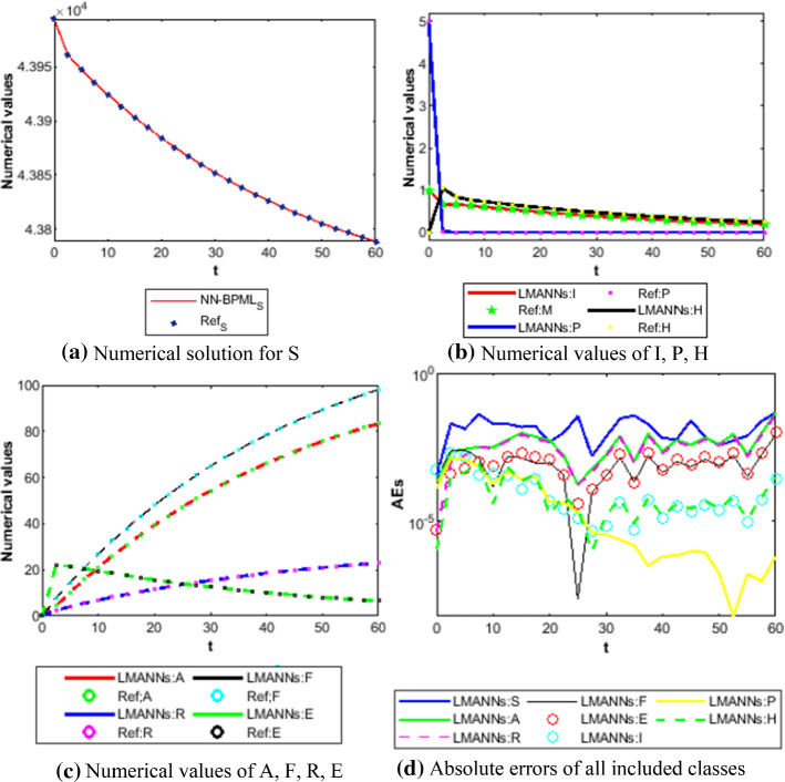
Therefore, the numerical and graphical results of LMANNs are determined for the susceptible class (S), export class (E), symptomatic and infectious class (I), infectious but asymptomatic class (A), super spreaders class (P), hospitalized (H), recovery class (R), fatality class (F) to explain the behavior corresponding to 60 days for each five case. Numerical outcomes are portrayed in Figs. 11, 12, 13, 14, 15, 16, 17, 18 and 19. The susceptible class (S) is graphically explains in subfigure 11a of case 1–4, the result values of S are lies in different ranges that is why subfigures for first four cases are shown that explains as more population higher susceptible class. The Figures 12a, 13a, 14a, 15a, 16a, 17a and 18a, describes graphically the behavior of E, I, P, A, H, R and F for case 1–4 of SEIPAHRF model for COVID-19 respectively. Fig. 19a–c explains the numerical results of all classes of SEIPAHRF model for COVID-19 for Wuhan city case 5 with reference solutions. The numerical values obtained by the proposed technique tabulated in Tables 3, 4, 5, 6 and 7 for all cases of each class of SEIPAHRF model for COVID-19.

Fig. 11.

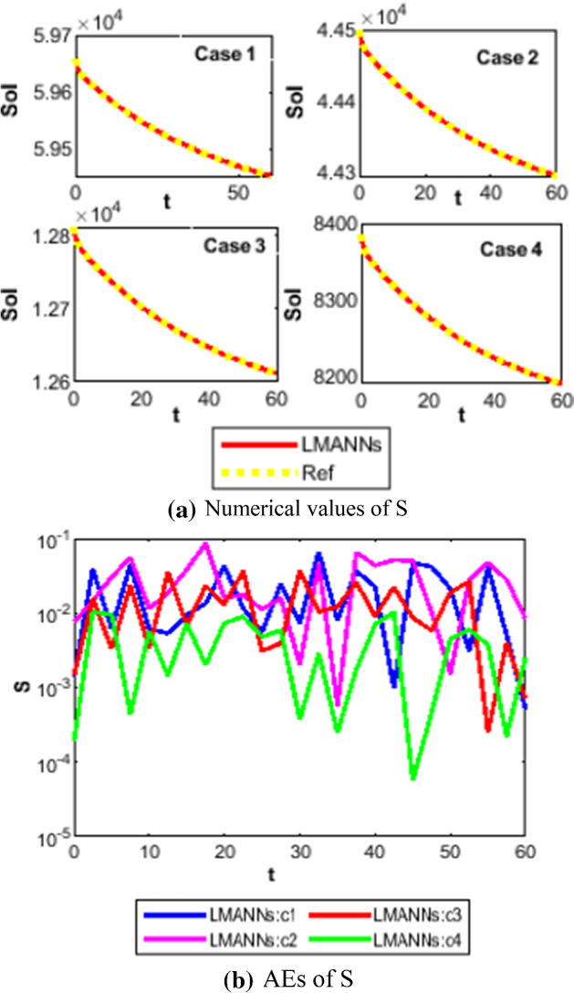
Comparison between proposed LMANNs with reference numerical results for susceptible class (S) of case 1–4

Fig. 12.

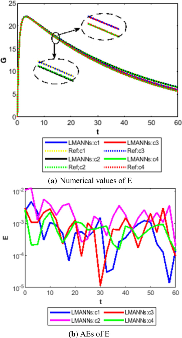
Comparison between proposed LMANNs with reference numerical results for export class (E) of case 1–4

Fig. 13.

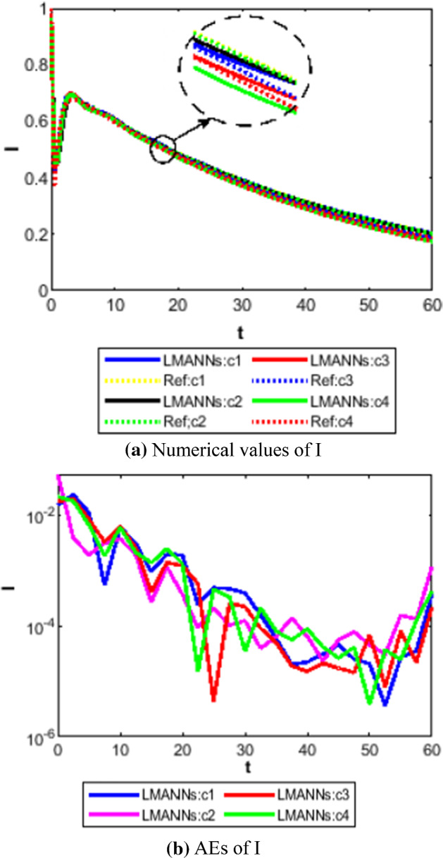
Comparison between proposed LMANNs with reference numerical results for symptomatic and infectious class (I) of case 1–4

Fig. 14.

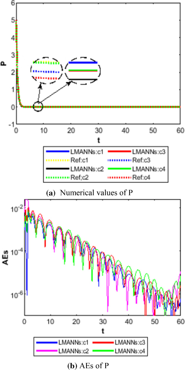
Comparison between proposed LMANNs with reference numerical results for super spreaders class (P) of case 1–4

Fig. 15.

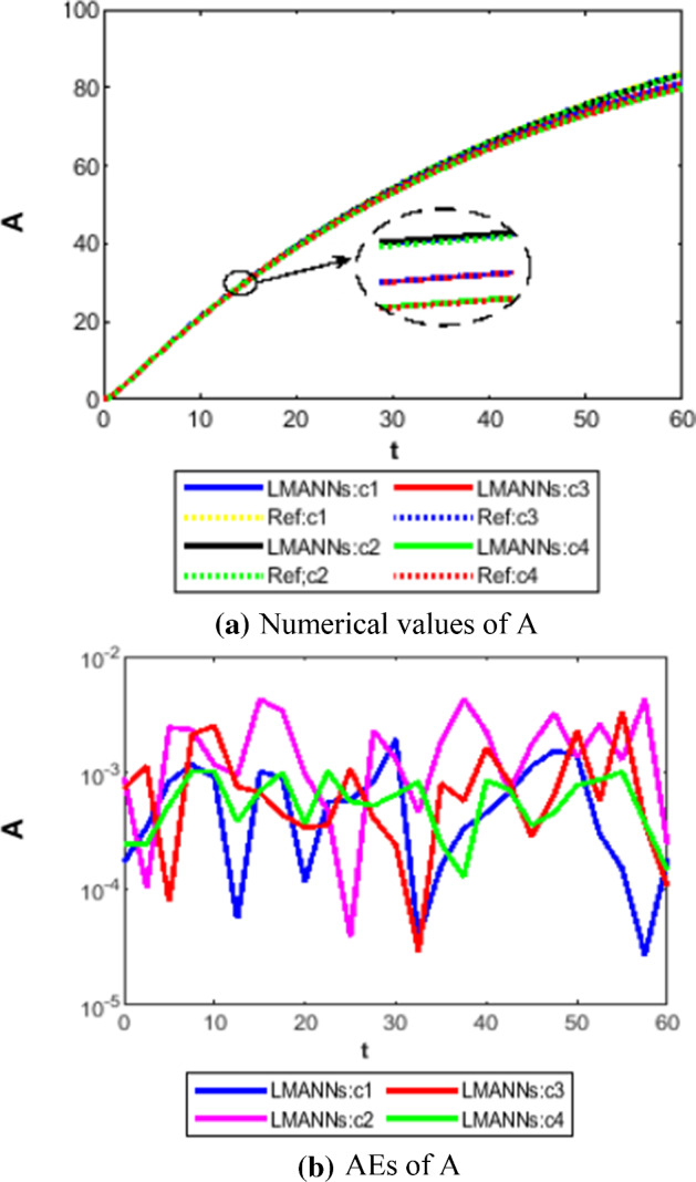
Comparison between proposed LMANNs with reference numerical results for infectious but asymptomatic class (A) of case 1–4

Fig. 16.

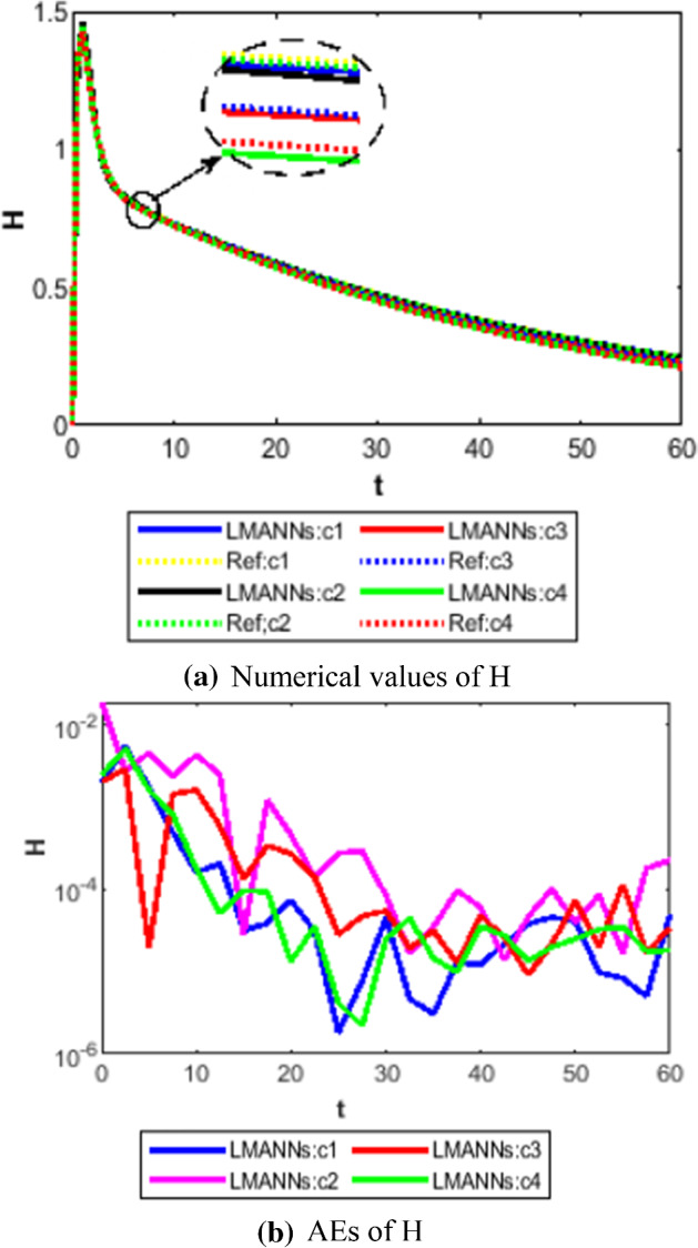
Comparison between proposed LMANNs with reference numerical results for hospitalized (H) of case 1–4

Fig. 17.

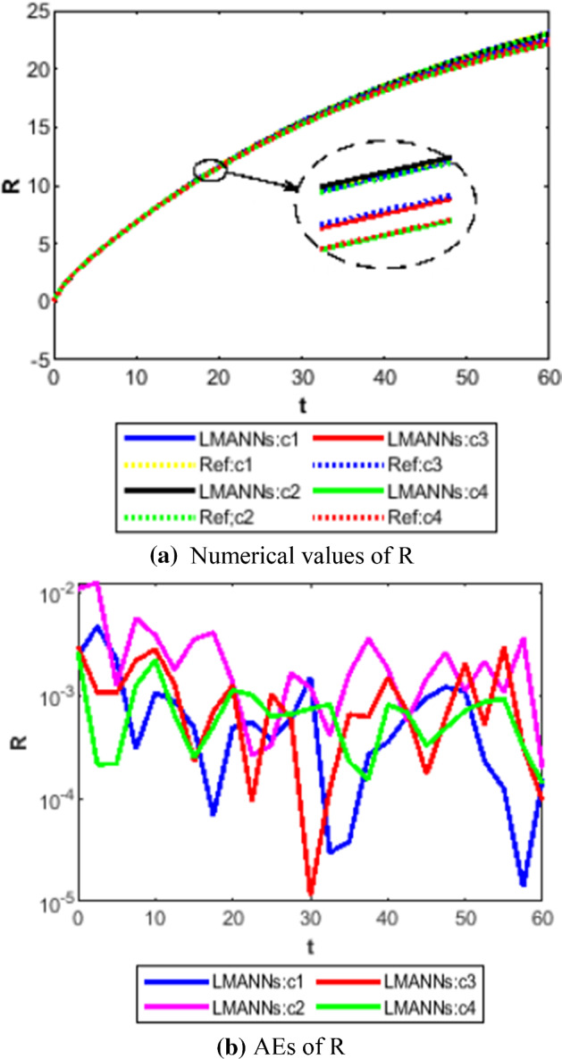
Comparison between proposed LMANNs with reference numerical results for recovery class (R) of case 1–4

Fig. 18.

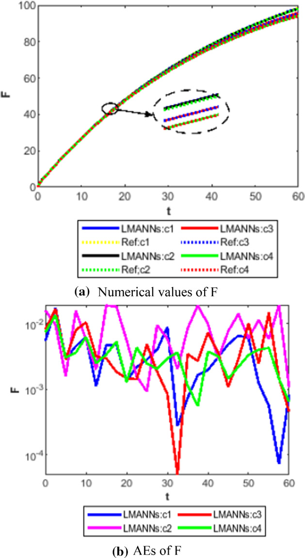
Comparison between proposed LMANNs with reference numerical results for fatality class (F) of case 1–4

Fig. 19.

Comparison between proposed LMANNs with reference numerical results for S, I, P, H, E, A, F, R and G of case 5

The obtained results through LMANNs matches with reference (ref) Adams numerical solutions in each case for all classes of SEIPAHRF model for COVID-19, therefore, in order to access the precision gauges, absolute errors (AEs) are determined. The AEs of all classes are presented in Figs. 11b, 12b, 13b, 14b, 15b, 16b, 17b and 18b for S, E, I, P, A, H, R, and F, respectively, for case 1–4 and tabular in Tables 8, 9, 10 and 11. AEs also satisfied the results of case 5 that is illustrated in Fig. 19d and tabular in Table 12. AEs of class S ranges between 10⁻⁰² and 10⁻⁰⁴ for cases 1, 3, 4, 5 and 10⁻⁰² to 10⁻⁰³ for case 2. Range of AEs for class A are 10⁻⁰³ to 10⁻⁰⁴ for cases 1, 3, 4, 10⁻⁰² to 10⁻⁰⁴ and 10⁻⁰² to 10⁻⁰⁶ for case 2 and 5, respectively. AEs of class R are 10⁻⁰³ to 10⁻⁰⁵ for case 1, 10⁻⁰³ to 10⁻⁰⁴ for case 2 to 4, and 10⁻⁰² to 10⁻⁰⁶ and for class F are 10⁻⁰³ to 10⁻⁰⁴, 10⁻⁰² to 10⁻⁰³, 10⁻⁰³ to 10⁻⁰⁴, 10⁻⁰³ to 10⁻⁰⁴, and 10⁻⁰² to 10⁻⁰⁴ of case 1–5, respectively. AEs are 10⁻⁰³ to 10⁻⁰⁵ of case 1, 3, 5 and, 10⁻⁰² to 10⁻⁰⁴ of case 2 and 10⁻⁰³ to 10⁻⁰⁷ of case 4 for class E. The range of AEs for class I, P and H are 10⁻⁰² to 10⁻⁰⁵, 10⁻⁰³ to 10⁻⁰⁷, 10⁻⁰³ to 10⁻⁰⁶ of case 1, 10⁻⁰² to 10⁻⁰⁵, 10⁻⁰³ to 10⁻⁰⁸, 10⁻⁰² to 10⁻⁰⁵ of case 2, 10⁻⁰² to 10⁻⁰⁵, 10⁻⁰³ to 10⁻⁰⁶, 10⁻⁰³ to 10⁻⁰⁶ of case 3, 10⁻⁰² to 10⁻⁰⁶, 10⁻⁰³ to 10⁻⁰⁸, 10⁻⁰³ to 10⁻⁰⁵ of case 4, 10⁻⁰³ to 10⁻⁰⁶, 10⁻⁰⁴ to 10⁻⁰⁷, 10⁻⁰⁴ to 10⁻⁰⁶ of case 5, respectively. These ranges of AEs for all classes of each case illustrates the accuracy of the proposed method that is up to 8 decimal places.

Table 8.

Absolute errors of case 1 against input day for all classes of SEIPAHRF model for COVID-19

Time	Case 1
	S	A	R	F	E	I	P	H
0	1.40E−03	9.79E−04	1.69E−04	5.48E−03	2.39E−03	1.50E−02	9.11E−04	1.97E−03
6	4.42E−02	3.89E−03	8.44E−05	4.08E−03	2.46E−03	1.05E−02	2.67E−03	5.28E−04
12	3.52E−02	1.25E−03	2.19E−04	1.68E−04	4.21E−04	1.40E−03	3.19E−04	1.81E−04
18	5.29E−03	1.10E−03	4.00E−04	1.92E−03	4.02E−05	8.37E−04	2.22E−04	7.64E−06
24	3.59E−02	2.22E−03	6.90E−04	3.34E−03	2.46E−04	8.92E−04	2.34E−04	1.53E−05
30	7.29E−03	7.59E−03	1.94E−03	8.92E−03	1.51E−03	3.88E−04	9.06E−05	4.53E−05
36	3.19E−02	3.94E−03	9.92E−04	4.52E−03	7.88E−04	1.06E−04	2.16E−05	2.72E−05
42	1.08E−02	1.43E−03	3.66E−04	1.68E−03	3.68E−04	2.94E−05	4.26E−06	1.26E−05
48	4.31E−02	5.40E−03	1.37E−03	6.17E−03	1.13E−03	2.75E−05	3.91E−07	4.40E−05
54	4.63E−02	7.12E−04	2.19E−04	8.17E−04	1.45E−04	3.23E−05	2.27E−07	9.05E−06
60	5.07E−04	7.29E−04	1.84E−04	8.36E−04	1.55E−04	3.79E−04	6.28E−07	4.92E−05

Table 9.

Absolute errors of case 2 against input day for all classes of SEIPAHRF model for COVID-19

Time	Case 2
	S	A	R	F	E	I	P	H
0	7.52E−03	1.98E−04	9.22E−04	1.62E−02	1.08E−02	5.39E−02	6.00E−03	1.89E−02
6	2.50E−02	3.09E−03	3.03E−03	9.03E−03	6.38E−03	7.81E−03	3.87E−03	8.99E−03
12	1.29E−02	5.74E−03	1.11E−03	8.74E−03	2.39E−03	1.12E−03	6.71E−04	1.48E−03
18	9.75E−03	1.00E−02	2.34E−03	1.28E−02	2.88E−03	8.80E−04	4.23E−04	9.37E−04
24	2.24E−02	7.97E−03	1.99E−03	9.69E−03	1.95E−03	3.63E−04	1.77E−04	3.72E−04
30	2.04E−03	5.08E−03	1.30E−03	5.94E−03	1.19E−03	1.23E−04	5.08E−05	8.35E−05
36	5.00E−02	4.70E−03	1.25E−03	5.32E−03	9.98E−04	1.48E−05	6.28E−06	5.03E−05
42	2.68E−02	8.30E−03	2.21E−03	9.51E−03	1.73E−03	4.26E−05	4.72E−06	7.69E−05
48	3.10E−02	1.12E−02	2.89E−03	1.28E−02	2.35E−03	6.58E−05	1.67E−06	9.19E−05
54	2.32E−02	1.41E−03	4.12E−04	1.66E−03	3.05E−04	4.50E−05	7.83E−08	2.30E−05
60	8.39E−03	9.73E−04	2.42E−04	1.07E−03	1.95E−04	1.16E−03	1.14E−05	2.26E−04

Table 10.

Absolute errors of case 3 against input day for all classes of SEIPAHRF model for COVID-19

Time	Case 3
	S	A	R	F	E	I	P	H
0	1.45E−03	3.80E−04	7.27E−04	8.17E−03	2.97E−03	1.75E−02	2.02E−03	2.05E−03
6	2.14E−02	5.61E−03	8.34E−04	3.39E−03	7.77E−03	1.30E−02	5.22E−03	2.81E−03
12	3.04E−02	3.74E−03	1.18E−03	5.27E−03	2.04E−04	1.21E−03	4.57E−04	2.55E−04
18	2.78E−02	8.32E−04	3.52E−04	1.37E−03	2.58E−04	6.40E−04	2.62E−04	1.63E−04
24	1.59E−02	4.66E−03	1.32E−03	5.72E−03	6.86E−04	5.46E−04	2.11E−04	1.59E−04
30	3.73E−02	6.29E−04	2.37E−04	8.55E−04	1.14E−05	2.22E−04	9.02E−05	5.50E−05
36	1.54E−02	3.42E−03	8.36E−04	3.90E−03	7.23E−04	7.24E−05	2.08E−05	3.91E−05
42	3.64E−02	4.34E−03	1.09E−03	4.89E−03	9.58E−04	3.67E−05	2.15E−06	3.70E−05
48	4.11E−03	8.28E−03	2.15E−03	9.43E−03	1.92E−03	5.22E−05	3.76E−06	7.06E−05
54	2.63E−02	9.67E−04	2.51E−04	1.18E−03	2.45E−04	1.31E−05	1.03E−06	7.83E−06
60	7.00E−04	4.24E−04	1.05E−04	4.56E−04	9.44E−05	2.16E−04	2.48E−06	3.46E−05

Table 11.

Absolute errors of case 4 against input day for all classes of SEIPAHRF model for COVID-19

Time	Case 4
	S	A	R	F	E	I	P	H
0	1.91E−04	1.00E−03	2.43E−04	7.44E−03	2.68E−03	2.11E−02	1.28E−03	2.47E−03
6	5.08E−04	2.65E−03	4.43E−04	5.36E−03	2.90E−03	9.42E−03	3.14E−03	2.59E−05
12	4.74E−03	2.53E−03	6.97E−04	3.49E−03	6.53E−04	4.83E−04	1.47E−04	1.19E−04
18	5.43E−04	1.23E−04	2.36E−04	1.63E−03	8.35E−04	1.79E−03	6.52E−04	5.82E−05
24	5.28E−03	1.29E−03	4.68E−04	2.16E−03	4.65E−07	7.69E−04	2.75E−04	3.31E−05
30	3.73E−04	2.60E−03	6.50E−04	2.97E−03	7.40E−04	3.46E−05	7.32E−06	2.54E−05
36	4.26E−03	3.21E−03	8.23E−04	3.64E−03	7.33E−04	9.02E−05	3.63E−05	1.73E−05
42	4.93E−03	3.73E−03	9.97E−04	4.26E−03	8.89E−04	2.87E−05	8.00E−07	3.30E−05
48	4.30E−03	1.28E−03	3.31E−04	1.42E−03	2.97E−04	1.00E−05	4.35E−06	9.27E−06
54	1.36E−02	4.14E−03	1.03E−03	4.71E−03	9.92E−04	6.69E−06	1.18E−08	3.54E−05
60	2.61E−03	5.63E−04	1.44E−04	6.48E−04	1.39E−04	4.26E−04	7.08E−06	1.82E−05

Table 12.

Absolute errors of case 5 against input day for all classes of SEIPAHRF model for COVID-19

Time	Case 5
	S	A	R	F	E	I	P	H
0	3.54E−04	4.51E−06	4.94E−06	2.39E−04	2.92E−04	5.12E−04	1.30E−04	1.13E−06
6	4.46E−02	3.59E−04	1.56E−04	5.55E−04	9.08E−04	1.49E−03	2.31E−04	4.77E−04
12	5.27E−03	6.42E−03	1.79E−03	6.97E−03	1.69E−03	3.82E−04	4.03E−04	6.52E−04
18	1.04E−03	7.68E−03	1.94E−03	9.03E−03	1.27E−03	2.58E−04	3.25E−04	3.66E−04
24	2.48E−02	3.92E−03	1.01E−03	4.46E−03	8.58E−04	2.45E−05	1.48E−05	4.61E−05
30	7.06E−03	1.54E−03	3.67E−04	1.76E−03	3.35E−04	7.31E−06	3.54E−06	1.66E−05
36	5.10E−04	9.78E−03	2.54E−03	1.12E−02	2.09E−03	6.43E−05	1.28E−06	7.79E−05
42	5.57E−03	2.69E−03	7.03E−04	3.03E−03	5.52E−04	1.74E−05	7.78E−07	2.15E−05
48	5.58E−03	2.38E−04	9.67E−05	2.86E−04	3.17E−05	1.27E−06	1.08E−06	2.04E−06
54	1.38E−03	3.15E−04	5.43E−05	3.40E−04	6.84E−05	2.45E−06	3.61E−07	2.46E−06
60	4.68E−02	3.94E−02	1.02E−02	4.49E−02	8.32E−03	2.55E−04	6.37E−07	3.12E−04

Conclusions

Artificial intellect based integrated computing intelligent platform is presented by means of neural networks with backpropagation of Levenberg-Marquard to find the solution of mathematical model SEIPAHRF for COVID-19 representing the spreading of Corona virus through different classes in the major cities of Pakistan and China for different cases that are constructed on the basis of real data. Dataset for SEIPAHRF model for COVID-19 is generated through Adams numerical solver for different classes. The 90%, 5% and 5% of the reference dataset is used as training, validation and testing for LMANNs. On the basis of above numerical study and investigation, following key findings of SEIPAHRF model for COVID-19 can be observed.

• Governing system of ODEs representing the radiative spread of COVID-19 are solved with the help of. LMANNs.

• Comparison of proposed results with reference numerical solution obtained through Adams method upto 8 decimal places which shows the accuracy and convergence of the proposed LMANNs.

• Aspect of the proposed method is further validated through numerical and graphical description based on convergence plots, error histogram, mean square errors and regression dynamics.

• Variants of parameter of interest greatly influence the dynamics of model SEIPAHRF.

• Performance of the computational process gets better for complexity in terms of time series, regression, histogram, MAE.

In future, one may implement proposed LMANN for solving the systems representing computer virus models [35, 36], prediction studies [37–41], nonlinear fractional differential equation [42, 43], bioinformatics models [44–46] and financial modeling [30, 47].

List of symbols

S[t]

Susceptible class

E[t]

Exposed class

I[t]

Infectious class of COVID-19 Epidemic

P[t]

Super propagation class

A[t]

Infectious but asymptomatic class

H[t]

Hospitalized class

R[t]

Recovery class

F[t]

Fatality class

δ_h

Death rate for hospitalized people

l

Relative transmissibility of hospitalized class

β

Transmission coefficient (infection)

β₁

Transmission coefficient (super spreaders)

k

Exposed to infectious rate

ρ₁

Exposed to infected rate

ρ₂

Exposed to super spreaders rate

γ_a

Rate of being hospitalized class

γ_i

Recovery rate without hospitalized

γ_r

Recovery rate of hospitalized patients

δ_i

Death rate due to infected people

δ_p

Death rate due to super spreaders

Compliance with ethical standards

Conflict of interest

The authors declare that they have no competing interests.

References

- 1.Gorbalenya AE, Baker SC, Baric RS, et al. The species severe acute respiratory syndrome-related coronavirus: classifying 2019-nCoV and naming it SARS–CoV-2. Nat. Microbiol. 2020;5:536–544. doi: 10.1038/s41564-020-0695-z. [DOI] [PMC free article] [PubMed] [Google Scholar]
- 2.Shereen MA, Khan S, Kazmi A, Bashir N, Siddique R. COVID-19 infection: origin, transmission, and characteristics of human coronaviruses. J. Adv. Res. 2020;24:91–98. doi: 10.1016/j.jare.2020.03.005. [DOI] [PMC free article] [PubMed] [Google Scholar]
- 3.Cui J, Li F, Shi ZL. Origin and evolution of pathogenic coronaviruses. Nat. Rev. Microbiol. 2019;17(3):181–192. doi: 10.1038/s41579-018-0118-9. [DOI] [PMC free article] [PubMed] [Google Scholar]
- 4.El Zowalaty ME, Järhult JD. From SARS to COVID-19: a previously unknown SARS-CoV-2 virus of pandemic potential infecting humans–Call for a One Health approach. One Health. 2020;9:100124. doi: 10.1016/j.onehlt.2020.100124. [DOI] [PMC free article] [PubMed] [Google Scholar]
- 5.Hughes JM, Wilson ME, Wilson SP, Gurley ES, Hossain MJ. Transmission of human infection with Nipah virus. Clin Infect. Dis. 2009;49(11):1743–1748. doi: 10.1086/647951. [DOI] [PMC free article] [PubMed] [Google Scholar]
- 6.Higazy M. Novel fractional order SIDARTHE mathematical model of the COVID-19 pandemic. Chaos Solitons Fract. 2020;138:110007. doi: 10.1016/j.chaos.2020.110007. [DOI] [PMC free article] [PubMed] [Google Scholar]
- 7.Tuan NH, Mohammadi H, Rezapour S. A mathematical model for COVID-19 transmission by using the Caputo fractional derivative. Chaos Solitons Fract. 2020;140:110107. doi: 10.1016/j.chaos.2020.110107. [DOI] [PMC free article] [PubMed] [Google Scholar]
- 8.Ivorra B, Ferrández MR, Vela-Pérez M, Ramos AM. Mathematical modeling of the spread of the coronavirus disease 2019 (COVID-19) taking into account the undetected infections. The case of China. Commun. Nonlinear Sci. Numer. Simul. 2020;88:105303. doi: 10.1016/j.cnsns.2020.105303. [DOI] [PMC free article] [PubMed] [Google Scholar]
- 9.Ng KY, Gui MM. COVID-19: development of a robust mathematical model and simulation package with consideration for ageing population and time delay for control action and resusceptibility. Phys. D Nonlinear Phenom. 2020;411:132599. doi: 10.1016/j.physd.2020.132599. [DOI] [PMC free article] [PubMed] [Google Scholar]
- 10.Khrapov P, Loginova A. Comparative analysis of the mathematical models of the dynamics of the coronavirus COVID-19 epidemic development in the different countries. Int. J. Open Inf. Technol. 2020;8(5):17–22. [Google Scholar]
- 11.Liu C, Wu X, Niu R, Wu X, Fan R. A new SAIR model on complex networks for analysing the 2019 novel coronavirus (COVID-19) Nonlinear Dyn. 2020;101(3):1777–1787. doi: 10.1007/s11071-020-05704-5. [DOI] [PMC free article] [PubMed] [Google Scholar]
- 12.Thomas DM, Sturdivant R, Dhurandhar NV, Debroy S, Clark N. A primer on COVID-19 mathematical models. Obesity. 2020 doi: 10.1002/oby.22881. [DOI] [PMC free article] [PubMed] [Google Scholar]
- 13.Rhodes T, Lancaster K. Mathematical models as public troubles in COVID-19 infection control: following the numbers. Health Sociol. Rev. 2020;29(2):177–194. doi: 10.1080/14461242.2020.1764376. [DOI] [PubMed] [Google Scholar]
- 14.Sardar T, Nadim SS, Rana S, Chattopadhyay J. Assessment of lockdown effect in some states and overall India: a predictive mathematical study on COVID-19 outbreak. Chaos Solitons Fract. 2020;139:110078. doi: 10.1016/j.chaos.2020.110078. [DOI] [PMC free article] [PubMed] [Google Scholar]
- 15.Liang K. Mathematical model of infection kinetics and its analysis for COVID-19. SARS and MERS. Infect. Genet. Evol. 2020;82:104306. doi: 10.1016/j.meegid.2020.104306. [DOI] [PMC free article] [PubMed] [Google Scholar]
- 16.Baleanu D, Mohammadi H, Rezapour S. A fractional differential equation model for the COVID-19 transmission by using the Caputo–Fabrizio derivative. Adv. Differ. Equ. 2020;2020(1):1–27. doi: 10.1186/s13662-019-2438-0. [DOI] [PMC free article] [PubMed] [Google Scholar]
- 17.Valenti VE, de Lemos Menezes P, de Abreu ACG, Vieira GNA, Garner DM. Social distancing measures may have reduced the estimated deaths related to Covid-19 in Brazil. J. Hum. Growth Dev. 2020;30(2):164–169. doi: 10.7322/jhgd.v30.10360. [DOI] [Google Scholar]
- 18.Zeb A, Alzahrani E, Erturk VS, Zaman G. Mathematical model for coronavirus disease 2019 (COVID-19) containing isolation class. BioMed Res. Int. 2020;2020:3452402. doi: 10.1155/2020/3452402. [DOI] [PMC free article] [PubMed] [Google Scholar]
- 19.Vespignani A, Tian H, Dye C, Lloyd-Smith JO, Eggo RM, Shrestha M, Scarpino SV, Gutierrez B, Kraemer MU, Wu J, Leung K. Modelling COVID-19. Nature Rev. Phys. 2020;2:279–281. doi: 10.1038/s42254-020-0178-4. [DOI] [PMC free article] [PubMed] [Google Scholar]
- 20.Giordano G, Blanchini F, Bruno R, Colaneri P, Di Filippo A, Di Matteo A, Colaneri M. Modelling the COVID-19 epidemic and implementation of population-wide interventions in Italy. Nature Med. 2020;26:855–860. doi: 10.1038/s41591-020-0883-7. [DOI] [PMC free article] [PubMed] [Google Scholar]
- 21.Naveed M, Baleanu D, Rafiq M, Raza A, Soori AH, et al. Dynamical behavior and sensitivity analysis of a delayed coronavirus epidemic model. Comput. Mater. Continua. 2020;65(1):225–241. doi: 10.32604/cmc.2020.011534. [DOI] [Google Scholar]
- 22.Bärwolff G. Mathematical modeling and simulation of the COVID-19 pandemic. Systems. 2020;8(3):24. doi: 10.3390/systems8030024. [DOI] [Google Scholar]
- 23.Ndairou F, Area I, Nieto JJ, Torres DF. Mathematical modeling of COVID-19 transmission dynamics with a case study of Wuhan. Chaos Solitons Fract. 2020;135:109846. doi: 10.1016/j.chaos.2020.109846. [DOI] [PMC free article] [PubMed] [Google Scholar]
- 24.Raja MAZ, Shah FH, Syam MI. Intelligent computing approach to solve the nonlinear Van der Pol system for heartbeat model. Neural Comput. Appl. 2018;30(12):3651–3675. doi: 10.1007/s00521-017-2949-0. [DOI] [Google Scholar]
- 25.Ahmad I, et al. Neuro-evolutionary computing paradigm for Painlevé equation-II in nonlinear optics. Eur. Phys. J. Plus. 2018;133(5):184. doi: 10.1140/epjp/i2018-12013-3. [DOI] [Google Scholar]
- 26.Masood Z, et al. Design of Mexican Hat Wavelet neural networks for solving Bratu type nonlinear systems. Neurocomputing. 2017;221:1–14. doi: 10.1016/j.neucom.2016.08.079. [DOI] [Google Scholar]
- 27.Ahmad I, et al. Novel applications of intelligent computing paradigms for the analysis of nonlinear reactive transport model of the fluid in soft tissues and microvessels. Neural Comput. Appl. 2019;31(12):9041–9059. doi: 10.1007/s00521-019-04203-y. [DOI] [Google Scholar]
- 28.Raja MAZ. Solution of the one-dimensional Bratu equation arising in the fuel ignition model using ANN optimised with PSO and SQP. Connect. Sci. 2014;26(3):195–214. doi: 10.1080/09540091.2014.907555. [DOI] [Google Scholar]
- 29.Mehmood A, et al. Design of neuro-computing paradigms for nonlinear nanofluidic systems of MHD Jeffery–Hamel flow. J. Taiwan Inst. Chem. Eng. 2018;91:57–85. doi: 10.1016/j.jtice.2018.05.046. [DOI] [Google Scholar]
- 30.Bukhari AH, et al. Fractional neuro-sequential ARFIMA-LSTM for financial market forecasting. IEEE Access. 2020;8:71326–71338. doi: 10.1109/ACCESS.2020.2985763. [DOI] [Google Scholar]
- 31.Mehmood A, Zameer A, Ling SH, et al. Integrated computational intelligent paradigm for nonlinear electric circuit models using neural networks, genetic algorithms and sequential quadratic programming. Neural Comput. Appl. 2019 doi: 10.1007/s00521-019-04573-3. [DOI] [Google Scholar]
- 32.Bukhari AH, et al. Design of a hybrid NAR-RBFs neural network for nonlinear dusty plasma system. Alex. Eng. J. 2020 doi: 10.1016/j.aej.2020.04.051. [DOI] [Google Scholar]
- 33.Sabir Z, et al. Neuro-heuristics for nonlinear singular Thomas–Fermi systems. Appl. Soft Comput. 2018;65:152–169. doi: 10.1016/j.asoc.2018.01.009. [DOI] [Google Scholar]
- 34.Raja MAZ, Shah FH, Alaidarous ES, Syam MI. Design of bio-inspired heuristic technique integrated with interior-point algorithm to analyze the dynamics of heartbeat model. Appl. Soft Comput. 2017;52:605–629. doi: 10.1016/j.asoc.2016.10.009. [DOI] [Google Scholar]
- 35.Masood Z, et al. Design of a mathematical model for the Stuxnet virus in a network of critical control infrastructure. Comput. Sec. 2019;87:101565. doi: 10.1016/j.cose.2019.07.002. [DOI] [Google Scholar]
- 36.Masood Z, et al. Design of epidemic computer virus model with effect of quarantine in the presence of immunity. Fundam. Inform. 2018;161(3):249–273. doi: 10.3233/FI-2018-1702. [DOI] [Google Scholar]
- 37.Zheng N, Du S, Wang J, Zhang H, Cui W, Kang Z, Yang T, Lou B, Chi Y, Long H, Ma M. Predicting covid-19 in China using hybrid AI model. IEEE Trans. Cyber. 2020;50(7):2891–2904. doi: 10.1109/TCYB.2020.2990162. [DOI] [PubMed] [Google Scholar]
- 38.Li L, Zhang Q, Wang X, Zhang J, Wang T, Gao TL, Duan W, Tsoi KKF, Wang FY. Characterizing the propagation of situational information in social media during covid-19 epidemic: a case study on weibo. IEEE Trans. Comput. Soc. Syst. 2020;7(2):556–562. doi: 10.1109/TCSS.2020.2980007. [DOI] [Google Scholar]
- 39.Jamshidi M, Lalbakhsh A, Talla J, Peroutka Z, Hadjilooei F, Lalbakhsh P, Jamshidi M, La Spada L, Mirmozafari M, Dehghani M, Sabet A. Artificial intelligence and COVID-19: deep learning approaches for diagnosis and treatment. IEEE Access. 2020;8:109581–109595. doi: 10.1109/ACCESS.2020.3001973. [DOI] [PMC free article] [PubMed] [Google Scholar]
- 40.Arora P, Kumar H, Panigrahi BK. Prediction and analysis of COVID-19 positive cases using deep learning models: a descriptive case study of India. Chaos Solitons Fract. 2020;139:110017. doi: 10.1016/j.chaos.2020.110017. [DOI] [PMC free article] [PubMed] [Google Scholar]
- 41.S. Hu, Y. Gao, Z. Niu, Y. Jiang, L. Li, X. Xiao, M. Wang, E.F. Fang, W. Menpes-Smith, J. Xia, H. Ye, Weakly supervised deep learning for covid-19 infection detection and classification from ct images. IEEE Access (2020)
- 42.Lodhi S, et al. Fractional neural network models for nonlinear Riccati systems. Neural Comput. Appl. 2019;31(1):359–378. doi: 10.1007/s00521-017-2991-y. [DOI] [Google Scholar]
- 43.Raja MAZ, Manzar MA, Shah SM, Chen Y. Integrated intelligence of fractional neural networks and sequential quadratic programming for Bagley–Torvik systems arising in fluid mechanics. J. Comput. Nonlinear Dyn. 2020;15(5):051003. doi: 10.1115/1.4046496. [DOI] [Google Scholar]
- 44.Umar M, et al. A stochastic computational intelligent solver for numerical treatment of mosquito dispersal model in a heterogeneous environment. Eur. Phys. J. Plus. 2020;135(7):1–23. doi: 10.1140/epjp/s13360-020-00557-8. [DOI] [Google Scholar]
- 45.Raja MAZ, Asma K, Aslam MS. Bio-inspired computational heuristics to study models of HIV infection of CD4+ T-cell. Int. J. Biomath. 2018;11(02):1850019. doi: 10.1142/S1793524518500195. [DOI] [Google Scholar]
- 46.Umar M, et al. Stochastic numerical technique for solving HIV infection model of CD4+ T cells. Eur. Phys. J. Plus. 2020;135(6):403. doi: 10.1140/epjp/s13360-020-00417-5. [DOI] [Google Scholar]
- 47.Ara A, et al. Wavelets optimization method for evaluation of fractional partial differential equations: an application to financial modelling. Adv. Differ. Equ. 2018;2018(1):8. doi: 10.1186/s13662-017-1461-2. [DOI] [Google Scholar]