Methane Emissions in a Chemistry‐Climate Model: Feedbacks and Climate Response

Abstract

Understanding the past, present, and future evolution of methane remains a grand challenge. Here we have used a hierarchy of models, ranging from simple box models to a chemistry‐climate model (CCM), UM‐UKCA, to assess the contemporary and possible future atmospheric methane burden. We assess two emission data sets for the year 2000 deployed in UM‐UKCA against key observational constraints. We explore the impact of the treatment of model boundary conditions for methane and show that, depending on other factors, such as CO emissions, satisfactory agreement may be obtained with either of the CH₄ emission data sets, highlighting the difficulty in unambiguous choice of model emissions in a coupled chemistry model with strong feedbacks. The feedbacks in the CH₄‐CO‐OH system, and their uncertainties, play a critical role in the projection of possible futures. In a future driven by large increases in greenhouse gas forcing, increases in tropospheric temperature drive, an increase in water vapor, and, hence, [OH]. In the absence of methane emission changes this leads to a significant decrease in methane compared to the year 2000. However, adding a projected increase in methane emissions from the RCP8.5 scenario leads to a large increase in methane abundance. This is modified by changes to CO and NOx emissions. Clearly, future levels of methane are uncertain and depend critically on climate change and on the future emission pathways of methane and ozone precursors. We highlight that further work is needed to understand the coupled CH₄‐CO‐OH system in order to understand better future methane evolution.

Key Points

• We study methane in present and future climate in a model employing flux‐based treatment of methane emissions

• We examine the source and importance of feedbacks in the CH₄‐CO‐OH system using a 0‐D box model and a 3‐D chemistry‐climate model

• We examine methane levels in future climate and the role played by climate and emissions changes

1. Introduction

Methane is an important greenhouse gas whose abundance in the atmosphere has changed dramatically over the course of the Earth's history (Quiquet et al., 2015). Mixing ratios of methane have increased significantly from pre‐Industrial era levels of around 750 ppb to ~1,850 ppb in 2018 (Loulergue et al., 2008). This growth, combined with the strong radiative efficiency of methane in the infrared, makes methane the second most important anthropogenic greenhouse gas, with an increase in radiative forcing from 1750 to 2011 of 0.48 ± 0.05 W m⁻² (IPCC, 2013). Unlike CO₂, the principal methane bands are not saturated so that its radiative forcing increases relatively more strongly with increases in concentration.

The atmospheric concentration of methane is a complex balance of its sources and sinks, both of which have large uncertainty. Furthermore, changes in its sources have an impact on the sinks. The sources are both natural and anthropogenic, including agricultural and natural wetlands, enteric fermentation in ruminant animals, fossil fuel extraction, landfill, and termites. Estimates of the combined anthropogenic emissions range from 275 Tg (CH₄) yr⁻¹ in CMIP5 (Lamarque et al., 2010) to 320 Tg (CH₄) yr⁻¹ in EDGAR vn4.2 (Janssens‐Maenhout et al., 2019), with biogenic emissions estimated between 177 and 284 Tg (CH₄) yr⁻¹ (Kirschke et al., 2013). Sinks comprise chemical losses, such as reaction with the hydroxyl radical, OH, and atomic chlorine in the troposphere, reaction with O¹D in the stratosphere, and biological losses, primarily uptake by methanotrophic microbes in soil. Expressed as the ratio of atmospheric burden to total losses, the present‐day atmospheric lifetime is 9.1 ± 0.9 yr (Prather et al., 2012), with a lifetime with respect to reaction with OH in the troposphere of between 10 and 11 years (Prinn et al., 2005). The majority (60%) of methane emissions occur in the Northern Hemisphere, but the long lifetime with respect to interhemispheric transport reduces the north to south (N:S) latitudinal gradient in methane to around 100 ppb.

A grand challenge in the field of atmospheric chemistry remains reconciling periods of pauses and growth in the methane record. The major complication arises from the fact that the uncertainties in both sources and sinks are large. In essence, it is possible to reconcile changes in methane by invoking changes in the source or sink terms within their uncertainties. The attribution of the variation in methane levels over the past two decades highlights many of these issues. Kirschke et al. (2013) examined trends over the past 30 years in atmospheric methane mixing ratios, focusing on emission estimates and their implementation in chemical transport models. They concluded that the uncertainties in biogenic and anthropogenic emissions as well as the model treatment of methane sinks and transport are important limitations on the ability to ascribe trends to changes in source or sink processes.

Future emissions of methane are inherently uncertain owing to uncertainty in socioeconomic scenarios, which determine the anthropogenic component, and changes and impacts of climate change, which control the natural component. The issue of future methane levels is further complicated given that the sinks for methane will also respond to climate change. Rising tropospheric temperatures will result in higher concentrations of water vapor in the atmosphere, and an increase in OH produced from the photolysis of ozone. However there is uncertainty about how atmospheric composition will change under climate change, particularly with regard to OH (Naik et al., 2013). Some model simulations suggest that OH may increase, but others suggest it is likely to decrease. A major cause of future simulated decreases in OH is increase in the abundance of CO, which is the major sink for OH in the atmosphere. CO itself is formed from the oxidation of CH₄ and so there is a complex, multifaceted, and uncertain set of processes which connect CO‐OH‐CH₄.

The interactions between ozone, its precursors, and methane are important to our understanding of future climate as both methane and ozone are radiatively active species, with the radiative impact of ozone between the pre‐Industrial period and the present day estimated at 0.40 W m⁻², similar in magnitude to that of methane (IPCC, 2013). Changes to methane emissions at the surface are also coupled to stratospheric composition via HOx chemistry, and future increases may cause increased stratospheric ozone destruction, with impact on the temperature structure and radiative budget.

Understanding the effect of future climate on methane levels therefore relies on models to provide a framework for a quantitative understanding of the emissions and factors controlling methane levels, particularly between methane and ozone, mediated by OH and CO. At present, there is a need to improve the process‐level treatment of methane emissions in the current generation of chemistry‐climate models. These mostly use a combination of latitude‐invariant lower‐boundary conditions (LBC) or latitude‐varying LBCs when available, constructed from scenarios. In the ACCMIP project, most models used some form of LBC, based on the Representative Concentration Pathways, with two using a uniform global mixing ratio and only one (LMDzOR‐INCA) applying emission fluxes. While these LBCs help maintain consistency across models by specifying the amount of methane at the surface, the adjustment to a prescribed mixing ratio serves as an additional source or sink of methane which may not be physically reasonable and is often not diagnosed or reported in the literature.

A more satisfactory modeling approach employs surface fluxes, ideally online, calculated at the process level, at the lower boundary of the atmospheric model. Flux methods are more physically based and can be directly connected to changes in land use, population, and other factors controlling emission. Methane emissions feed back onto oxidants, and an interactive chemistry scheme is required to capture the interactions between the methane and oxidants such as OH. The complexity this introduces was recently discussed by (Gaubert et al., 2017) who indicated that optimization of methane emissions using offline OH oxidants or linearized chemistry schemes introduces systematic errors due to missing feedbacks in the linear chemistry scheme. Indeed, at present, there are significant differences between the OH field calculated in the current generation of chemistry‐climate models and reference OH climatologies, such as Spivakovsky et al. (2000), or observationally derived constraints, such as mean OH mixing ratio (Prinn et al., 2005), the N:S OH gradient (Patra et al., 2014) and methane lifetime (Prather et al., 2012). In general, models are high‐biased in OH, so that methane lifetimes are around 10% lower than observational constraints (Voulgarakis et al., 2013), and show a hemispheric N:S OH gradient greater than unity, whereas observations suggest an approximately equal amount of OH in both hemispheres (Patra et al., 2014).

The sources of these differences are unclear, but the need remains to develop CCMs capable of representing the distribution of methane accurately. The radiative forcing due to methane is the result of the distribution of methane throughout the atmosphere, and assessment of the radiative forcing due to methane necessitates the use of a model capable of representing the combined effect of anthropogenic emissions and other forcings, and the interaction between these changes, on methane levels and its radiative effect. For this purpose, CCMs remain the most suitable tool.

Hence, there is a clear need to go beyond the LBC‐based treatments and to investigate the methane budget within a CCM, while recognizing the structural uncertainties which pertain in any CCM. We here assess methane emissions, and attempt to improve agreement between model and observations, within the framework of a coupled chemistry‐climate model, UM‐UKCA (O'Connor et al., 2014). We do not attempt to necessarily reproduce the “correct” methane budget. Rather, our approach is to derive an emission data set which is consistent with our model, which itself includes our best approximation to an atmospheric chemistry scheme within its dynamical/radiative framework and includes the important feedback processes. We will then explore how these feedbacks, and any uncertainties, affect the model projection of possible futures.

We explore these ideas using a range of models from simple to complex, focusing on the impact of feedbacks. Section 2 uses a simple box model to investigate the nature of these feedbacks. In section 3 we use a 3‐D model and flux‐based emissions to examine the interactions between methane, OH, and species including CO and ozone. For the present day (sections 3.2 and 3.3), we explore three scenarios focusing on the uncertainty in methane and CO emissions and the impact of these on methane mixing ratios at the surface. For future climate (section 4), we use RCP8.5 to quantify the effect of individual components of climate change on atmospheric composition and the interactions between them. Finally, to understand the effect of different lower boundary conditions, we compare a flux‐based emissions scheme against the ACCMIP multimodel mean for RCP8.5, which is largely composed of models employing LBC methane.

2. Feedbacks in the CH₄‐CO‐OH System in Box Model Simulations

To guide the development of an emission‐based lower boundary condition, we first explore the global methane burden using a simplified single‐box model and a representative chemical mechanism (Prather, 1996), as described by the equations below.

$$\frac{\mathit{d}\left[{\mathit{CH}}_4\right]}{\mathit{d}t}=S_{\mathit{CH}4}-k_1\left[\mathit{OH}\right]\left[{\mathit{CH}}_4\right]$$ (1)

$$\frac{\mathit{d}\left[\mathit{CO}\right]}{\mathrm{dt}}=S_{\mathit{CO}}-k_2\left[\mathit{OH}\right]\left[\mathit{CO}\right]+k_1\left[\mathit{OH}\right]\left[\mathit{C}{\mathit{H}}_4\right]$$ (2)

$$\frac{d\left[\mathit{OH}\right]}{\mathit{d}t}=S_{\mathit{OH}}-k_x\left[\mathit{OH}\right]-k_2\left[\mathit{OH}\right]\left[\mathit{CO}\right]-k_1\left[\mathit{OH}\right]\left[\mathit{C}{\mathrm{H}}_4\right]$$ (3)

Figure 1 shows the results of four simulations with this simple model designed to illustrate aspects of the behavior of methane in the chemistry‐climate system. For our base scenario, we employed methane, CO and OH emissions representative of the lower atmosphere for the year 2000— $S_{C{H}_4}$(methane emissions) of 540 Tg (CH₄) year⁻¹, S_CO (CO emissions) of 1,370 Tg (CO) yr⁻¹ and an OH source (S_OH) of 1.15 × 10⁶ molecules cm⁻³ s⁻¹, similar to the values used in (Prather, 1994) (with the mass of the CH₄ and CO emissions mixed across the whole atmosphere (atmospheric mass 5.18 × 10¹⁸ kg) and k _x = 1 s⁻¹). Here, we were interested to examine the impact of methane emissions on methane concentrations, the methane feedback, and to quantify the methane feedback factor.

Figure 1.

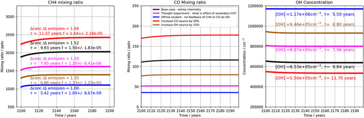
Box model studies of interactions between (left) CH4 , (middle) CO, and (right) OH. Black line = base scenario; Blue line = scenario 1: no feedback; Red line = scenario 2: enhanced primary CO emissions; magenta line scenario 3: no secondary CO formation via methane oxidation; Brown line = scenario 4: increased OH source. Left‐hand panels include perturbation lifetimes (as in Prather, 1994) divided by feedback factor, f. Right‐hand panels show lifetime with respect to reaction with OH.

The methane feedback, as mentioned in section 1, arises because increases in methane, and its oxidation product, CO, decrease the concentration of the major oxidant, OH, and so extend the methane lifetime. The feedback factor, f, is defined as the ratio of fractional change in methane concentration, m, to the fractional change in methane emissions, E,

$$f=\frac{\raisebox{1ex}{$\mathrm{\Delta }m$}\!\left/ \!\raisebox{-1ex}{$m_0$}\right.}{\raisebox{1ex}{$\mathrm{\Delta }E$}\!\left/ \!\raisebox{-1ex}{$E_0$}\right.}$$ (4)

Following Holmes (2018), we can similarly derive the feedback factor from the transient response during model spin‐up to steady state (see below).The simulations were performed as described in Table 1. The box model was initialized with zero concentration of all species and integrated forward for 100 years to reach steady state. The box model was then restarted with the methane source term having been increased by 5% and integrated forward in time for another 100 years, so that the concentrations tend toward a new steady state value. The results of these second simulations are shown in Figure 1.

Table 1.

Overview of Box Model Simulations

Simulation name	$S_{C{H}_4}$ Tg (CH4) yr−1	SCO Tg (CO) yr−1	SOH cm−3 s−1	Feedbacks	${\tau }_{C{H}_4+\mathit{OH}}$ yr	f
Base (Black)	540	1,370	1.15 × 106	Full	9.84	1.5
Scenario 1 (Blue)	540	1,370	1.15 × 106	None	5.50	1
Scenario 2 (Red)	540	2055	1.15 × 106	Full	11.70	1.64
Scenario 3 (Magenta)	540	1,370	1.15 × 106	No 2o CO	7.96	1.2
Scenario 4 (Brown)	540	1,370	1.44 × 106	Full	7.25	1.36

Figure 1a shows the response of the base model to a change in methane emissions of 5% (black line). Over the course of 40 years, the methane mixing ratio increases from 1,890 ppb to a new value of 2,030 ppb, ~7.6% higher than the original value and larger than expected on the basis of the change in methane emissions. The increase in methane, in excess of the 5% increase in the emissions, is due to the feedback of methane on the OH sink. Using Equation 4, this change in concentration gives a feedback factor, f, of 1.52, which agrees well with the retrieved value of f of 1.50 from a fit of the transient behavior and with values derived from CCMs and CTMs (range 1.4 to 1.7; Holmes, 2018; Fuglestvedt, 1999). Fgure 1b shows the transient CO response, in which there is a small increase in CO mixing ratio due to secondary CO production from methane oxidation and to suppression of the OH that is also a CO sink. Figure 1c shows a decrease in OH in the base run of around 2% or 1.5 × 10⁴ molecules cm⁻³. The methane lifetime (defined as the reciprocal of k₁[OH]) of 9.8 years agrees well with the lifetime derived from the fit of the transient behavior of 9.9 years and the observational estimates for reaction with tropospheric OH of 11.2 ± 0.9 years (Prather et al., 2012).

Figure 1 also shows the results of four other box model sensitivity experiments. In Scenario 1, shown as a blue line, we remove entirely the chemical feedbacks in the system (f = 1). This is similar to global model integrations in which the model oxidants might be specified (e.g., to TransCom‐VSLS; Hossaini et al., 2016, and others). In Scenario 2, the red line, the size of the primary CO source was increased by 50%, reflecting the large uncertainty in primary emissions and secondary CO production. Scenario 3, shown in magenta, was performed in which secondary CO production from methane oxidation is suppressed (that is, the third term on the right‐hand side in Equation 2 is removed). A fourth integration (Scenario 4), shown in brown, details the effect of increasing the OH source term by 25%.

Scenario 1 shows that, in the absence of chemical feedbacks (blue lines), methane mixing ratios increase linearly with methane emissions, as expected, and a feedback factor of 1 is retrieved. Lower methane mixing ratios and a much shorter methane lifetime (5.4 years) are observed than in the other cases, due to the higher levels of OH in the system. Responses in CO and OH are instantaneous and no transient behavior is observed in these integrations.

In Scenario 2, when primary CO emissions are increased (red line in Figure 1), there is a concomitant increase in methane mixing ratios. The effect of the increased CO emissions is to suppress OH and thus elevate methane mixing ratios. For this simple model system, the 50% increase in CO emissions results in a 56% increase in CO mixing ratio, and an increase in methane mixing ratios of ~20%. We recover a feedback factor of 1.64 and a methane lifetime of around 11.7 years. OH decreases by 15% and CH₄ increases by ~20%. This scenario examines the possibility that CO emissions are low biased or that secondary CO formation from VOC oxidation is under‐represented. In the latter case, Griffin et al. suggest that this may amount to a contribution of 45 ppb to CO levels locally, which would be around 50% (Griffin et al., 2007).

Scenario 3 shows intermediate behavior between the “zero” feedback case and the base run. There is a smaller suppression of the OH sink, compared to base, as the removal via reaction with secondary CO is now absent. The overall decrease in CO is ~60 ppb or 50%, and OH is higher by 1.5 × 10⁵ cm⁻³. The higher OH gives lower methane levels and a shorter methane lifetime compared to base, and a lower feedback factor of 1.2.

Finally, an increase in OH source (Scenario 4, brown line) yields, as expected, decreases in CH₄ and CO with respect to base. A 25% increase in OH source leads to an ~35% increase in OH concentrations.

Taken together, smaller feedback factors, f, compared to base, are observed in Scenarios 1, 3, and 4, while Scenario 2 shows a higher feedback factor. In Scenario 2, the effect of increased CO emissions is to suppress OH and the CH₄ sink which leads to larger increases in methane mixing ratio per unit increase in methane emissions. In Scenarios 3 and 4, the changes lead to increases in OH and enhancement of the chemical sink, and so there are smaller increases in methane mixing ratios as the emissions increase. These integrations illustrate that the feedback factor may be modified by changes to any one of the methane, CO and OH sources, including secondary CO production.

This simple model indicates some of the difficulties present when trying to model atmospheric methane. Although the scheme is highly simplified, it is clear that representing the complex feedbacks in the atmospheric system will be important. We find a 50% difference in lifetime between runs with and without feedback; depending on the feedback included, lifetimes range between about 8 and 12 years. It is also clear that constraining emissions using observations and a model with fixed oxidants is likely to be an unsatisfactory approach.

Having made these general points, we consider emissions, specific to our global model, further in the next section.

3. Evaluation of Candidate Methane Emissions Fields in a Chemistry‐Climate Model

In this section we consider candidate scenarios, quantifying the impact of our flux‐based methane emissions scheme on the burden and distribution of key tropospheric species including CH₄, ozone and OH (sections 3.1 and 3.2). We examine the interactions between these species and, in section 3.3, briefly compare the impact of a flux‐based scheme to a mixing ratio‐based lower boundary treatment.

We examine the performance of two methane emissions estimates, one based on EDGAR and the other on CMIP5 emissions data, in the UM‐UKCA model, in order to assess their suitability for subsequent modeling studies. As indicated above, the implementation of a flux‐based methane emissions scheme in the current generation of chemistry‐climate models is made challenging by both the uncertainty in recent emissions estimates, the range of possible model metrics and the difficult in assessing the effect of biases in oxidants such as OH and ozone in the underpinning model (Patra et al., 2014), (Gaubert et al., 2017).

3.1. Model Configuration and Emissions Data Sets

Our global chemistry‐climate model uses version 7.3 of the Met Office's Unified Model HadGEM3‐A (Hewitt et al., 2011) coupled with the United Kingdom Chemistry and Aerosol scheme (hereafter referred to as UM‐UKCA). The model is run in atmosphere‐only mode with a horizontal resolution of 2.5° latitude by 3.75° longitude, 60 vertical levels up to 84 km, and prescribed sea surface temperatures and sea ice extents. We use SST, sea ice and other forcings appropriate for the year 2000, and use perpetual year 2000 “time‐slice” experiments, with the model run to steady state over a period of at least 50 years. Emissions of species other than methane are given in Table 2 and are based on the CMIP5 emissions data set. Climatologies of our results are constructed from the final 10 years of model data. The model chemistry scheme is based on the combined stratospheric‐tropospheric chemistry scheme (Archibald et al., 2020. The scheme includes extensive treatment of tropospheric and stratospheric chemistry. A total of 71 tracers (75 species) react in 56 photolysis, 200 bimolecular, 24 termolecular, and 5 heterogeneous reactions. These include the Ox (O and O₃), HOx, and NOx chemical cycles and the oxidation of CO, ethane, propane, and isoprene, stratospheric chlorine and bromine chemistry, including heterogeneous processes on polar stratospheric clouds and liquid sulfate aerosols. Photolysis rates are calculated interactively by the Fast‐JX scheme (as implemented in Telford et al., 2013) and ozone is coupled interactively between chemistry and radiation. Methane, nitrous oxide, chlorofluorocarbons, and similar gases (e.g., hydrochlorofluorocarbons) use a prescribed mixing ratio in the radiation code. Aerosols are calculated with the Coupled Large‐scale Aerosol Simulator for Studies in Climate (CLASSIC) aerosol scheme (Appendix A, Bellouin et al., 2011). Uniform mixing ratios are assumed for H₂ (34.528 ppb) and CO₂ according to the simulated climate.

Table 2.

Emission Fluxes Used in the Year 2000 Time Slice Integrations Derived From EDGAR‐TRANSCOM (See Text)

NOx	138	Tg NO2 yr−1
CH4	548	Tg CH4 yr−1
CO	1,113	Tg CO yr−1
HCHO	9	Tg HCHO yr−1
C2H6	27	Tg C2H6 yr−1
C3H8	14	Tg C3H8 yr−1
Me2CO	46	Tg Me2CO yr−1
CH3CHO	9	Tg CH3CHO yr−1
Isoprene	573	Tg C yr−1
MeOH	121	Tg C yr−1

Before considering the methane emissions in UM‐UKCA, we can get a first, simple picture of the required distribution of those emissions using a simplified “two‐box” model of the atmosphere, with first‐order transport connecting the Northern and Southern Hemispheres which we may use to inform the development of more detailed emissions fields suitable for use in a 3‐D chemistry climate model. Our analytical model treats methane as a single species with a global average lifetime of 8.7 ± 0.3 years based on observations (Prather et al., 2012), and a lifetime with respect to interhemispheric transport of 1.2 years. This gives an analytical expression for NH and SH methane levels whose emissions can be adjusted to reproduce the observed average methane tropospheric concentration in each hemisphere and the hemispheric gradient. With our selected lifetime, annual emissions of 400 Tg CH₄ in the NH and 185 Tg CH₄ in the SH result in a mean mixing ratio of 1,840 ± 70 ppb and a N:S gradient of 100 ppb, which are in broad agreement with our more detailed analysis below.

Informed by this simple calculation and the chemistry box model results discussed in section 2, we performed three UM‐UKCA integrations in an attempt to compare and optimize methane emissions in our model. In the first experiment (BASE), we used an emissions data set based on EDGAR anthropogenic emissions (Janssens‐Maenhout et al., 2019) and Transcom‐CH₄ for biogenic emissions (total including soil sink 548 Tg (CH₄) yr⁻¹), as detailed in Table 3. In the second (ΔCO), we used the same EDGAR+Transcom‐CH₄ emissions, but increased total CO emissions by 50% globally from the AR5 emissions, while in the final experiment (ΔEMS) we used a methane data set based on the CMIP5 emissions and a modified biogenic emissions data set, with total emissions of 585 Tg (CH₄) yr⁻¹, as optimized in an earlier version of UM‐UKCA by Heimann (2017).

Table 3.

BASE Versus ΔEMS Methane Emissions

Source	Strength/Tg		ΔEMS‐BASE
	BASE	ΔEMS	Tg	Percentage
Anthropogenic	322	275	−49	−15%
Biomass burning	35	25	−10	−29%
Wetlands	190	259	−69	+36%
Other biogenic	26	26	0	0
Total	548	585	+37	+7%

For BASE, the anthropogenic emissions, namely fossil fuels, rice, animals, waste, and others, were taken from the EDGAR database for the year 2000, and amount to 322 Tg (CH₄) yr⁻¹ or about 56% of total present‐day methane emissions. Emissions from transportation and energy production amount to 30 Tg. A seasonal variation is applied to the CH₄ emissions from the fossil fuels coal and gas, which has been shown to improve comparison to observational data (Gurney et al., 2005; Heimann, 2017). Seasonally varying biomass burning emissions are taken from the GFED 3 database but scaled to 35 Tg (CH₄) yr⁻¹ to match recent estimates (Kirschke et al., 2013). In this experiment, the wetland emissions used originate from the TransCom‐CH₄ project (Patra et al., 2011). Their geographical distribution and their seasonal cycle is based on the NASA Goddard Institute of Space Studies inventory, but the individual wetland emissions types (bogs, swamps, and tundra) have been scaled as stated in Patra et al. (2011) to a global flux of 149 Tg (CH₄) yr⁻¹. Finally, the global wetland emission flux has been uniformly increased to match the average wetland emission flux, as estimated in the wetland CH₄ intercomparison of models project (WETCHIMP; Melton et al., 2013), giving total wetland emissions of 190 Tg (CH₄) yr⁻¹. The methane hydrate (6 Tg (CH₄) yr⁻¹) and termite (20 Tg (CH₄) yr⁻¹) emissions are seasonally invariant, while soil oxidation (25 Tg (CH₄) yr⁻¹) is included as a negative emission (sink) with no seasonal cycle (Fung et al., 1991). Figure 2 shows the distribution of methane emissions (not including soil sink processes, so the total is 573 Tg (CH₄) yr⁻¹) in the BASE experiment.

Figure 2.

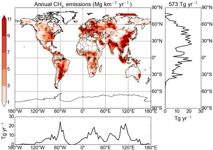
Distribution of methane emissions (Tg (CH4) per year) in the BASE experiment.

For the second integration, ΔCO, we increased the CO emissions globally by 50%, similar to one of the chemistry box model calculations in section 2, to a total of 1,660 Tg CO yr⁻¹. All other emissions were as in BASE.

For the third experiment, ΔEMS, we used a second methane emissions data set with a slightly greater total emissions and a slightly different spatial distribution. All other nonmethane emissions were kept as in BASE. We adopted the anthropogenic methane emissions from the Coupled Model Intercomparison Project Phase 5 (CMIP5) data set (Lamarque et al., 2010) and total 275 Tg CH₄ yr⁻¹. CMIP5 recommendations were also followed for the biomass burning emissions, which are seasonally varying and total 25 Tg CH₄ yr⁻¹ (van der Werf et al., 2017). Table 3 summarizes the breakdown of emissions by sector in BASE and ΔEMS.

As CMIP5 does not make recommendations for natural emissions, we chose to implement wetland emissions from a second source, in this case the ORCHIDEE data set described in Melton et al. (2013). This provides tropical wetland fluxes of 187 Tg (CH₄) yr⁻¹ and boreal wetland fluxes of 72 Tg (CH₄) yr⁻¹, giving a total of 259 Tg (CH₄) yr⁻¹, 28% of which come from the northern extratropics, in line with the upper end of data from the WETCHIMP Intercomparison (Melton et al., 2013). Emissions from methane hydrates and termites used data from Fung et al. (1991). Further details are given in Heimann (2017). The emissions total 585 Tg CH₄ yr⁻¹, with ~77% in the Northern Hemisphere, which compares favorably with the estimate from our simple “two‐box” model of total emissions at 585 Tg CH₄ yr⁻¹, with ~68% of emissions in the NH.

Figure 3 shows the difference in the methane emissions between ΔEMS and BASE. Anthropogenic emissions in ΔEMS are 15% lower than in BASE, while wetland emissions have increased by 36%, their strength nearly equalling the total strength of all anthropogenic emissions in ΔEMS. The distribution of emissions is also slightly different: Emissions are slightly stronger in the tropics and weaker in norther midlatitudes, compared to BASE. The development of the ΔEMS emissions data set is described in more detail in Heimann (2017), but serves as a second, plausible candidate emissions data set for study. We do not suggest that either emissions distribution is a priori better than the other.

Figure 3.

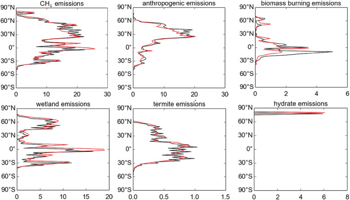
Latitudinal variation in annual methane emissions data sets used in these experiments, in Tg (CH4) per year. Black: BASE, red: ΔEMS.

3.2. Simulations of Methane Concentrations in Coupled Chemistry Experiments

Both methane flux emission data sets perform well in UM‐UKCA. Table 4 summarizes global mean quantities of interest in our three integrations. Figure 4 shows the latitudinal distribution of methane, CO and OH, compared to observations or other assessments where these are available. For CH₄ and CO we used NOAA surface measurements, averaged between January 2000 and December 2005 (Dlugokencky et al., 2019), and the model is sampled at the equivalent station position, while for OH we compared to a reference climatology (Spivakovsky et al., 2000) and to the ACCMIP multimodel mean as given in Naik et al. (2013).

Table 4.

Summary Table of the Results of Year 2000 Perturbed Emissions Experiments

	BASE	ΔCO	ΔEMS
Tropospheric CH4 emissions/Tg (CH4) per year	548	548	585
Tropospheric CO emissions/Tg (CO) per year	1,113	1,660	1,113
Whole atmospheric CH4 burden/Tg (CH4)	4,325	4,790	4,789
Tropospheric global mean CH4/ppb	1,590	1787	1760
N:S methane mixing ratio gradient/ppb	104 vs. 97 (obs)	105	103
Tropospheric OH/105 molecules cm−3	12.4	11.1	12.0
Tropospheric global mean CO/ppb	77 vs. 102 (obs)	107	81
N:S CO mixing ratio gradient/ppb	39 vs. 67 (obs)	59	38
OH + CH4 flux/Tg (CH4) yr−1	526	521	580
TauOH + CH4/years	8.2	9.2	8.6
Ozone burden/Tg	331	329	336
Feedback factor, f	1.55	Not done	Not done

Figure 4.

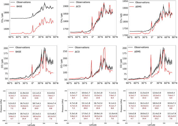
Outcome of the integrations: (left‐hand panels) BASE (methane emissions + CMIP5 anthropogenic CO, NOx, etc); (middle panels) ΔCO, as above but CO emissions increased by 50% with respect to CMIP5 estimates; (right‐hand panels) ΔEMS, CMIP5 methane emissions + anthropogenic CO, NOx. (top row) CH4 mixing ratio versus observations; (middle row) CO mixing ratio vs observations; (bottom row) OH distribution (/105 cm⁻³) versus literature estimates (top row: UKCA experiments, second row: ACCMIP multimodel mean, bottom row: Spivakovsky).

For the BASE experiment, an interhemispheric gradient in methane of 104 ppb is calculated, compared with the observed 97 ppb, but with a global mean methane mixing ratio of 1,590 ppb, which is low biased by 190 ppb (11%) compared to NOAA surface measurements of 1,780 ppb, and lower than the value of 1,840 ppbv returned from our analytical model. This suggests that either the tropospheric methane sink (mainly OH) is too strong in BASE or that the methane emissions are too low.

As we have discussed above, in a chemistry‐climate model such as UM‐UKCA, it is difficult to independently adjust species, such as OH, which are under the control of in situ secondary sources and sinks. By increasing CO, however, we increase the size of the global OH sink term which provides some control. Figure 4b shows the results of the integration ΔCO in which CO emissions were increased by 50%. There is now good agreement both in terms of modeled CH₄ and CO, with both species showing acceptable global means and latitudinal gradients. The strong feedback between CH₄, CO, and OH is illustrated in this run by the simultaneous increase in CO and CH₄ and a suppression of OH from 1.2 to 1.1 × 10⁶ cm⁻³.

The ΔCO results are consistent with a low‐bias in the primary emissions or in secondary CO production in BASE. The global increase in CO emissions, while leading to improved comparison with observations at most latitudes, reduces agreement between model CO and observation in the regions of highest emissions, such as northern midlatitudes (see Figure 4, middle panel), which might suggest that the low bias in BASE in other regions is due to missing CO production in the model, most likely from missing higher VOC sources, rather than an underrepresentation of primary emissions.

Figure 4 shows that using higher methane emissions, increased from 548 Tg in BASE to 585 Tg in ΔEMS, leads to improved agreement between modeled and measured methane, in terms of its global mean mixing ratio (modeled 1,760 ppb vs. observed 1,780 ppv) while maintaining a good N:S latitudinal gradient (103 ppb vs 97 ppb observed), and CO and OH levels similar to the BASE run. Peak CO mixing ratios are better represented in this experiment, in comparison with ΔCO, while global mean mixing ratio remains low biased. From Table 3 it may be inferred that the improved agreement for methane arises from a decrease in anthropogenic emissions, which is located primarily in NH midlatitudes, and an increase in biogenic sources, mainly in the tropics (Heimann, 2017). The N:S gradient is similar in all three integrations.

The three experiments demonstrate the challenge of developing and refining CH₄ emissions estimates in a global chemistry‐climate model incorporating the strong chemical feedbacks as outlined in section 2. The tight chemical coupling between CH₄, CO, and OH means that the global suppression of the OH radical by increased methane emissions feeds back further by decreasing the size of the methane sinks and so increases the CH₄ lifetime. These changes propagate throughout the chemical system via other coupled chemical pathways.

For these experiments involving year 2000 forcings, the feedback from a 6.7% increase in methane emission strength between the BASE and ΔEMS experiments leads to a 10.7% increase in methane burden and mean surface mixing ratio, giving a feedback factor of 1.55 (very similar to the result we obtained with our simple model in section 2). However, a global increase in CH₄ emissions, while expected to remove the low bias in global mean mixing ratio found in the BASE experiment, would also modify the N:S gradient, as the sink for methane in NH midlatitudes is less strong than in the tropics, where the OH is larger. Comparing BASE to ΔEMS we find that an emission set involving stronger tropical sources gives the best agreement in terms of mean surface mixing ratio and the N:S gradient. Our results show that these two quantities provide suitable criteria for assessment and optimization of emissions with respect to observations. However, the system is underconstrained, and so we cannot say that these results show the ΔEMS emissions data set to be the only suitable candidate. Indeed, the BASE emissions data set would also be acceptable, provided a set of stronger CO emissions were used alongside (i.e., from ΔCO). Our goal here is not to establish which of these two sets is more correct, but to highlight that these emissions indicate a consistency within the model framework, making them suitable for further study in our CCM, UM‐UKCA. In the following section we compare the model using the three emission scenarios with results derived under the conditions of a fixed lower boundary mixing ratio.

3.3. Implications of the CH₄‐CO‐OH System on Tropospheric Composition

In this section we compare our UM‐UKCA results from the ΔEMS integration with those from Banerjee et al. (2016). That study used a latitude‐invariant methane mixing ratio based lower‐boundary condition, appropriate to the year 2000, and emissions for other species as in ΔEMS. As such, the essential difference between the runs lies in the methane lower boundary condition.

The impact of the different boundary conditions is shown in Figure 5 which shows the zonally averaged methane distribution difference between ΔEMS and LBC, with methane in the ΔEMS experiment as contour lines, and the percentage difference with respect to LBC as filled contours, that is, as ΔEMS − LBC. The higher methane emissions in the NH in ΔEMS with respect to those implied by the latitude‐invariant LBC lead to the largest methane enhancements near the surface, but an increase with respect to LBC is observed throughout the NH troposphere. Conversely, there are lower amounts of methane in ΔEMS in the SH, as emissions in ΔEMS are lower there than the effective emissions in LBC. The largest changes are observed at high latitudes in the NH, where there are significant local sources, but the impact is observed at the 1–2% level throughout the NH troposphere. It would appear that the opposite impact is observed in the stratosphere, where methane levels are higher in the ΔEMS integration (see also Winterstein et al., 2019, who find a similar result).

Figure 5.

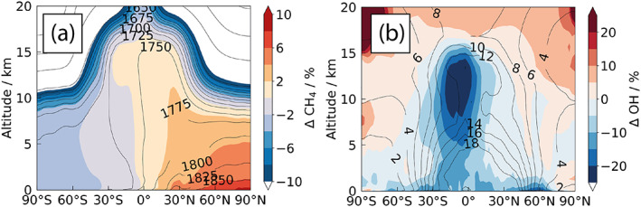
(a) Impact of methane boundary condition treatment on annual average zonal mean methane mixing ratios, shown as ΔEMS − LBC. (b) Impact of methane boundary condition treatment on OH. Contour lines show (a) methane mixing ratio (ppb) and (b) [OH] (10⁵ cm⁻³) in ΔEMS, with differences, as ΔEMS − LBC, as filled regions.

Figure 5b shows that the impact of the different boundary conditions on OH is small but also complex. In the free troposphere, CH₄ acts as a sink for OH leading to lower levels of OH. The greatest impact of the higher methane mixing ratios is seen in the tropical upper troposphere, with the largest changes in OH seen south of the equator near the tropical tropopause, where the increase in the OH sink is strongest.

The impact on tropospheric ozone of the differences in the methane boundary conditions is minor. Throughout the tropical troposphere O₃ changes are of the order of 1 ppb, which is around 2 – 3% and similar to the variation observed between integrations here. Global tropospheric ozone increases from 329 Tg in LBC to 336 Tg in ΔEMS, a similar 2% increase, presumably due to higher levels of methane in the upper tropical troposphere, which result in higher levels of methane‐derived peroxy radicals in the region where ozone production by lightning NOx is dominant.

The effect on the methane lifetime of the different treatments of the methane lower boundary conditions, including changes in emissions, is summarized in Figure 6. For comparison purposes, data from the ACCMIP experiments are shown (Naik et al., 2013). The figure shows that only a few of the ACCMIP models lie within the bounds of observational constraints of global mean OH and methane lifetime, with the majority having higher OH and hence shorter methane lifetime. UM‐UKCA results also lie outside the observational constraints but close to the range provided by ACCMIP (Voulgarakis et al., 2013). The strong feedbacks between CH₄ and OH ensure that the higher CH₄ emissions in ΔEMS lead to lower global mean OH and hence longer CH₄ lifetime. Given the good agreement between modeled and measured surface methane, the figure supports the possibility that OH sinks in the free troposphere are underrepresented in the current generation of chemistry‐climate models, which would lead to these models having higher OH and lower methane lifetime. Our experiments with increased CO sources would support this, and suggest that an improved treatment of CO production from shorter‐lived VOC is crucial to improving model bias in OH and methane lifetime.

Figure 6.

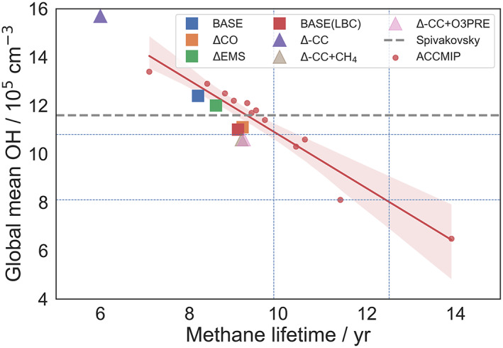
Variation in methane lifetime across experiments. Dashed vertical and horizontal lines reflect the observationally determined constraints on the methane lifetime. The red solid line shows a linear regression to the ACCMIP data, with shading indicating 95% confidence limits.

4. Chemistry‐Climate Interactions in the CH₄‐CO‐OH System

The previous section has highlighted the importance of feedbacks in the CH₄‐CO‐OH system. Model‐based approaches to balancing the contemporary methane budget must recognize the interdependence of emissions and the chemical feedbacks. When we consider the future, emissions of methane and CO later this century are very uncertain and changes in temperature, humidity, ozone precursors, and the stratospheric ozone column will all have a role to play in driving changes in methane concentrations. In this section, we describe a second set of CCM experiments, designed to illustrate the coupling of these different changes on methane.

We focus specifically on a set of simulations using the CMIP5 anthropogenic emissions data set for the year 2100. We use this as a basis for a study of the role of chemistry‐climate interactions involving methane, focusing on the RCP8.5 scenario. We use an atmosphere‐only configuration of UM‐UKCA, employing methane emissions but otherwise similar to that described in Banerjee et al. (2016). The model is forced by sea ice and SST fields derived from separate coupled atmosphere‐ocean integrations using HadGEM3 and concentrations of ozone depleting substances (ODS) and greenhouse gas (GHG) concentrations (CO₂, methane [in the radiation scheme, see next] nitrous oxide, chlorofluorocarbons, and hydroclorofluorocarbons) representative of year 2100 under the RCP8.5 scenario. Under these conditions, interactively simulated lightning NOx emissions increase from 7 (year 2000) to 11 Tg(N) yr⁻¹.

For these experiments, ozone was passed interactively between the chemistry and radiation schemes. However, the methane mixing ratio used in the radiation scheme was imposed following RCP8.5 at its 2100 mixing ratio and differs from the methane calculated using the coupled chemistry scheme and emissions, as discussed next. In this way, the physical climate factors controlling the OH oxidant field (with the exception of ozone) are kept constant between integrations. This is similar to the procedure followed by Banerjee et al. (2016).

In RCP8.5, there are large changes to physical climate (as a result of the large GHG forcing) and significant changes to both ozone precursors and to methane emissions. For example, NOx and CO emissions decrease significantly, while there are large increases in anthropogenic methane emissions from the energy, agriculture, and landfill sectors, and small decreases in biomass burning emissions. Following the RCP protocol, only anthropogenic methane emission increases are included, with the distribution and strength for the natural components (wetlands, termites, and hydrates) assumed to be identical to the present day. Table 5 lists the emissions used in these experiments. NOx and CO emissions decrease significantly compared with Year 2000, modifying both ozone and OH. Acetone, isoprene, and methanol emissions increase slightly, while those of other (less abundant) hydrocarbons decrease.

Table 5.

RCP8.5 Emissions Fluxes Used in the One‐at‐a‐Time Year 2100 Time‐Slice Integrations

Species	Emissions	Strength
CH4	1,170	Tg CH4 yr−1
CO	734	Tg CO yr−1
HCHO	5	Tg HCHO yr−1
C2H6	17	Tg C2H6 yr−1
C3H8	8	Tg C3H8 yr−1
Me2CO	49	Tg Me2CO yr−1
CH3CHO	6	Tg CH3CHO yr−1
Isoprene	580	Tg C yr−1
MeOH	129	Tg C yr−1

Note. See text for details of the changes in each experiment.

We performed one‐at‐a‐time future perturbations in order to attribute responses to changes in emissions or other forcings, outlined in Table 6. In each experiment, one forcing was increased in line with the RCP8.5 pathway. The first, ΔCC, examined the impact of physical climate change on atmospheric composition, by including only the effect of changes under RCP8.5 to the climate forcers, with all emissions affecting chemical composition (methane, ozone precursors, etc.) held at year 2000 values. The second experiment, Δ(CC + CH₄), again uses the 2100 GHG mixing ratios to force the climate state but now with increased anthropogenic methane emissions driving changes in atmospheric composition via the coupled CH₄‐CO‐OH system. For the third experiment, we again used the RCP8.5 climate scenario, as well as changes to both ozone precursor and anthropogenic methane emissions. This third experiment results in an integration comparable to the ACCMIP RCP8.5 time slice performed by a variety of chemistry‐climate models.

Table 6.

Summary of the Year 2100 Perturbed Emissions Experiments

Experiment	Climate forcers	Anthropogenic CH4 emissions	Biogenic CH4 emissions	O3 Preemissions
ΔCC	2100	2000	2000	2000
Δ (CC + CH4)	2100	2100	2000	2000
Δ(CC + EMS)	2100	2100	2000	2100 (RCP8.5)

While RCP8.5 is clearly not the only possible scenario of interest, it is a useful test case for understanding the relative importance of the factors controlling future methane levels and the study of feedbacks between emissions and composition changes. In addition to following a well‐defined pathway, our aim for these integrations is to allow the study of changes to both physical climate and chemical emissions on methane, OH and ozone, and to begin to attribute their impact on other components of the chemistry‐climate system.

Table 7 and Figures 7, 8, 9 present results. We plot zonal means of species over the last 10 years of a time slice integration for conditions corresponding to year 2100 in the different RCP8.5 pathways.

Table 7.

Summary of the Results of Year 2100 Perturbed Emissions Experiments

	ΔCC	Δ(CC + CH4)	Δ(CC + EMS)
Tropospheric CH4 emissions/Tg (CH4) yr−1	585	1,170	1,170
Tropospheric CO emissions/Tg (CO) yr−1	1,113	1,113	734
Anthropogenic NOx emissions/Tg N yr−1	44	44	30
Whole Atmospheric CH4 burden/Tg (CH4)	3,421	10,336	10,260
Tropospheric global mean CH4/ppb	1,275	3,828	3,746
Tropospheric OH/105 molecules cm−3	15.7	10.5	10.6
OH + CH4 flux/Tg (CH4) yr−1	568	1,120	1,121
Tau(OH + CH4) /years	6.0	9.2	9.2
Tropospheric O3 burden/Tg	350	443	427
Feedback factor, f	1.62	1.44	1.43

Figure 7.

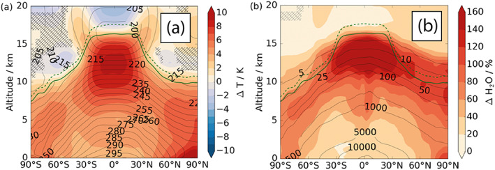
Changes to zonal mean temperature and water vapor concentration in RCP8.5 2100 shown as ΔCC‐ΔEMS. Contour lines show (a) temperature (K) and (b) H₂O (ppb) in ΔEMS, with differences, as ΔCC‐ΔEMS as filled regions.

Figure 8.

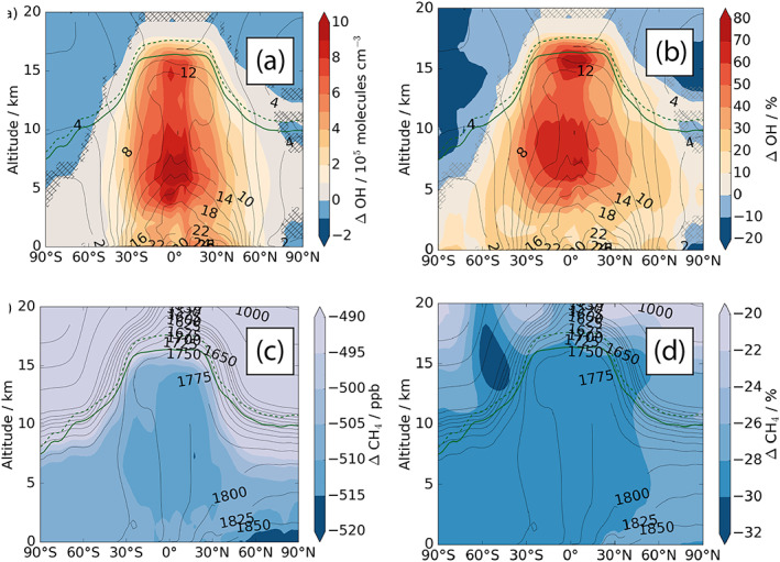
(upper panel) Absolute (a, 10⁵ molecules cm⁻³) and relative (b, %) changes in annual mean zonally averaged OH (ΔCC with respect to year 2000). The contour lines show the absolute OH concentrations for year 2000 (10⁵ molecules cm⁻³). (lower panel) Absolute (c, ppb) and relative (d, %) changes in annual mean zonally averaged methane (ΔCC − ΔEMS). The contour lines in (b) show the absolute methane mixing ratios for ΔEMS (ppb). Hatched areas are not significant at the 95th level according to the Student's t test. The tropopause for the ΔEMS (ΔCC) experiment is depicted in all figures as the solid (dashed) dark green line.

Figure 9.

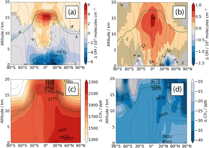
(upper panel) Changes in annual mean zonally averaged OH concentrations (10⁵ molecules cm⁻³). (a) Δ(CC + CH4) − ΔEMS; the contour lines show the absolute OH concentrations for ΔEMS (10⁵ molecules cm⁻³); (b) Δ(CC + EMS) − Δ(CC + CH4). On the left, the contour lines show the absolute OH concentrations for year 2000 (10⁵ cm⁻³), on the right, the contour lines show the absolute OH concentrations for Δ(CC + CH4). (lower row, c) Changes in annual mean zonally averaged methane mixing ratio. Δ(CC + CH4) − ΔEMS; (d) Δ(CC + EMS) − Δ(CC + CH4); On the left, the contour lines show the absolute CH4 mixing ratios for year 2000 (ppb), on the right, the contour lines show the absolute CH4 mixing ratios for Δ(CC + CH4).

Climate change results in a warmer atmosphere capable of sustaining greater concentrations of water vapor, which, together with higher lightning NOx emissions, leads to an increase in OH production rates throughout the troposphere. In ΔCC, the troposphere warms with increases in surface temperature of between 2 and 10 K (Figure 7a), with corresponding increases in water vapor concentration throughout the troposphere (Figure 7b).

Given that the emissions of the OH sink species, CH₄ and CO, are unchanged, the changes in water vapor and temperature result in an increase in global mean OH from 10.5 × 10⁵ molecules cm⁻³ to 15.7 × 10⁵ molecules cm⁻³. Figures 8a and 8b show that this increase is largest in the tropics, where humidity increases are largest, and in the free troposphere where the ozone precursor of OH responds sensitively to increases in LNOx.

Figures 8c and 8d show the corresponding change in methane mixing ratios. Under these conditions, the total atmospheric methane burden decreases to 3,421 Tg (CH₄) which is 1,368 Tg (CH₄) (29%) smaller than the year 2000 ΔEMS burden. Despite the burden reduction, the absolute flux through the reaction between methane and OH in ΔCC remains as high as in Base (568 Tg (CH₄) yr⁻¹ and 560 Tg (CH₄) yr⁻¹, respectively), consistent with the system being in steady state. The burden reduction, combined with the high flux of methane loss with tropospheric OH, leads to a reduction of the methane lifetime to 6.2 years, 2.5 years (30%) shorter than the ΔEMS lifetime. The reduced lifetime is the result both of increased OH and an increased rate of the OH + CH₄ reaction at higher temperatures.

Next, Figure 9 shows the results from the Δ(CC + CH₄) and Δ(CC + EMS) experiments. Tropospheric OH concentrations in both runs are reduced by around 50% compared to ΔCC, and are less than in ΔEMS, indicating that the decrease in OH caused by the emission changes outweighs the increase in OH caused by changes to the physical climate. Compared to ΔCC, there is a dipole pattern to the change in OH. There is an increase in OH in the region of enhanced LNOx emissions, while near the surface, where emissions of the CH₄ sink species are higher, a reduction in OH is seen (more pronounced in Δ(CC + EMS)). The large increase in OH throughout the upper troposphere seen in ΔCC is suppressed in the lower and mid troposphere but, especially in Δ (CC + CH4), is not completely offset in the tropical tropopause layer region.

The increased methane emissions, which significantly reduce OH (Figure 9a) and decrease the tropospheric oxidative capacity, lead to an increase in methane levels, as seen in Figure 9c. The doubling of methane emissions in the RCP8.5 scenario increases the atmospheric methane burden to 10,336 Tg (CH₄) in the Δ (CC + CH4) experiment. This is 5,547 Tg (CH₄) (116%) larger than in the year 2000 ΔEMS integrations and 6,915 Tg (CH₄) (202%) larger than in ΔCC. Figure 9c shows that the largest increases in methane in the Δ(CC + CH₄), and Δ(CC + EMS) experiments are found in the lowermost troposphere between the equator and 60°N, coincident with the largest methane emission increases in this region.

Figure 10 summarizes the effect of these experiments on ozone. Changes to the physical climate and ozone precursors yield changes to the tropospheric ozone burden of opposite sign, and (coincidentally) of nearly equal size. The role of anthropogenic methane emissions is clearly seen—the approximate doubling of methane emissions moving from ΔCC to Δ(CC + EMS) from 585 to 1,170 Tg leads to an increase in ozone burden of around 25% from 350 to 427 Tg.

Figure 10.

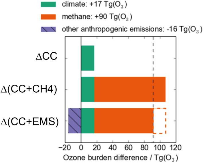
Changes to tropospheric ozone burden in the RCP8.5 experiments.

The methane lifetime derived with respect to tropospheric OH loss increases from 6.0 years in ΔCC to 9.2 years for the Δ(CC + CH₄) and Δ(CC + EMS) experiments. The Δ(CC + EMS) lifetime lies at the lower end of the ACCMIP multimodel lifetime estimate for the year 2100 (10.5 ± 1.6 years; Voulgarakis et al., 2013). Figure 11 compares the all‐forcing RCP8.5 experiment, Δ(CC + EMS), for year 2100, with some of the recent ACCMIP experiments. There is good agreement with the mean of the ACCMIP experiments that predominantly used an LBC methane condition, but the profile of CH₄ is slightly different, particularly in the upper troposphere, where the emissions‐based scheme produced the largest changes in OH and where the sensitivity of radiative forcing will be largest.

Figure 11.

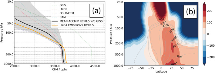
(a) Methane profile in RCP8.5 experiments. (b) Differences with respect to the ACCMIP multimodel mean CH4 in ppb. Contours show the ACCMIP multimodel mean, filled contours show the difference as Δ(CC + EMS)‐ACCMIP.

Taken together, these integrations allow us to attribute the effect of the various changes contained within our RCP8.5 scenarios. First, the ΔCC experiment shows that the changes to the physical climate produced by the large increases in radiative forcing lead to large increases in temperature and humidity, as expected. These serve to increase OH levels and suppress methane. Second, the Δ(CC + CH₄) experiment shows that the projected increases in methane emissions in this pathway lead to lower OH and increased methane lifetime. Finally, in the Δ(CC + EMS) integration, which is equivalent to the ACCMIP RCP8.5 experiments (Lamarque et al., 2013), the change in ozone precursors, CO and NOx, have little effect on either OH or ozone (with, e.g., the effect of the decrease in CO emissions being compensated by increased oxidation of CH₄) and the overall changes in RCP8.5 are driven mostly by the large increase in methane. Table 7 shows that compared to year 2000, and incorporating all changes, there is an approximate doubling of methane burden by 2100 in RCP8.5 scenario and an approximate 100 Tg increase in ozone, with little overall change in OH levels.

As Figures 8 and 9 show, the response of atmospheric composition to changes in methane emissions is quite heterogeneous and is driven in different locations by different controlling factors. The effect of climate forcing is important; in all experiments, there is an increase in OH in the upper troposphere, driven by local humidity changes and increased ozone production from lightning NOx, but at the surface the sign of the change in OH depends sensitively on the strength of methane emissions. In ΔCC, there is an increase in OH at the surface driven by increased humidity, while in Δ(CC + CH₄) and Δ(CC + EMS), the surface OH has decreased significantly as the result of larger OH sinks provided by the increased methane levels. The magnitude of the change in methane mixing ratio also varies strongly across the troposphere in different experiments. In Δ(CC + CH4), the largest methane increases are seen in the Northern Hemisphere high latitudes, where annually‐averaged oxidation is less efficient due to seasonal variation in OH, with particularly low OH in winter, and the lower temperatures in these regions, compared to lower latitudes, suppresses the rate of chemical oxidation.

It is clear from the above that there are significant regional variations in the response of composition to the various emission changes in RCP8.5. The strength of the methane emission feedback on concentration is therefore not expected to be constant throughout the atmosphere. To explore this we performed separate 3‐D experiments for each scenario following a 5% increase in methane emissions so as to derive feedback factors, which are reported in Table 7. These are calculated from the transient behavior of the global methane burden as the model spins up toward a new steady state, as in Holmes (2018). There is small but significant variation between the various experiments. In ΔEMS, the feedback factor is 1.55, which in ΔCC increases to 1.62, but decreases in the Δ(CC + CH₄) and Δ(CC + EMS) experiments to 1.43 and 1.44, respectively. The differences in the global‐mean feedback are difficult to attribute unambiguously, given the strong spatial variation in the response of methane mixing ratio to (spatially varying) changes in methane emissions.

The changes to methane burden and the feedback factors in these experiments can be compared with results from the box model, which we introduced in section 2. To guide understanding we performed a second set of box model integrations using scenarios based on the RCP8.5 experiments described above, the results of which are shown in Figure 12.

Figure 12.

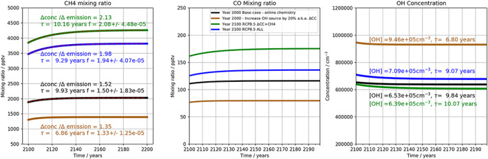
Box model studies of interactions between (left) CH4, (middle) CO, and (right) OH. Brown/black lines: Scenarios 1 and 4 are plotted from Figure 2. Green line: Scenario 5: Increased OH source and CH4 emissions increased to 1,170 Tg. Blue line: Scenario 6 based on RCP8.5.

Figure 12 shows the results from the base box model run (black lines) and Scenario 4 (brown lines) from Table 1 as comparisons for understanding the new box model simulations. Scenario 4, with a 30% increase in [OH], now approximates our ΔCC experiment in which OH sources are increased following an increase in humidity. The green line in Figure 12 shows Scenario 5, used to represent Δ (CC + CH₄), in which both the OH source is increased by 25%, as in the proxy for ΔCC, and the methane emissions are increased by a factor of 2, including the increase in anthropogenic emissions to 1,170 Tg. The blue line in Figure 12 shows Scenario 6, in which methane emissions are increased as in Scenario 5, but CO emissions are decreased to 783 Tg and the OH source remains at 25% above the year 2000 base scenario. This aims to replicate our Δ(CC + EMS) RCP8.5 integrations using UM‐UKCA.

In Scenarios 4–6, final methane mixing ratios of 1,390, 4,260, and 3,820 ppb are calculated, reflecting the variation in CH₄ seen across the ΔCC, Δ(CC + CH4), and Δ(CC + EMS) experiments using UM‐UKCA, where global mean mixing ratios of 1,275, 3,828, and 3,746 ppb, respectively, were found. In the box model, the changes in feedback factor between the different scenarios are larger than in UM‐UKCA, being 1.33, 2.13, and 1.98 across Scenarios 4–6, behavior which follows the combined response to the variation in OH sources and sinks between the experiments. In Scenario 4, the increased OH source term effectively suppresses the response to increases in CH₄ emissions, leading to a smaller change in methane mixing ratio for a given change in methane emissions (5% in these integrations) and a lower feedback factor. In Scenario 5, the increase in CH₄ emissions, despite the larger OH source term, strongly suppresses OH, giving a decrease of nearly 50%, and ensures that a 5% emissions change leads to a significantly higher relative increase in methane mixing ratios. In Scenario 6, the decrease in CO emissions leads to enhanced OH and a less strong methane feedback factor of 1.98. The agreement between box and 3‐D model, particularly in Scenario 6, is encouraging and supports the analysis above in terms of the importance of OH sources and sinks in controlling methane concentration. In fact, similar box model experiments with a lower OH source (taken from the base box model case) were not able to produce such good agreement, indicating the importance of the simultaneous increases in OH source and decrease in CO emissions. The variation in feedback factor between experiments is much stronger than calculated in the 3‐D model, where additional transport, temperature, and climate effects partially mitigate the effect of emissions changes and where spatial variations also play an important role. Clearly, the feedbacks in the 3‐D model are also more buffered than in the box model, and the variation is less strong across experiments. Similar behavior was observed by Holmes (2018), who found only a small variation across a range of emissions scenarios in 3‐D model experiments.

In summary, the CO‐OH‐CH₄ system response is strongly coupled and responds sensitively and nonlinearly to future changes in OH sources and sinks as well as CO and CH₄ emissions. Understanding the strength of these couplings is important for our understanding of methane concentrations and their radiative effects in future climate.

5. Summary and Conclusions

The tight coupling and feedbacks in the CH₄‐CO‐OH system have been investigated using a hierarchy of models. We have assessed the impact of changes in emissions of carbon monoxide and methane and of the background climate state using box models and the UKCA chemistry‐climate model. We find that significant challenges arise in trying to disentangle the drivers of change in the system.

Tropospheric abundances of methane and CO mixing ratios and tropospheric [OH] were investigated in a series of experiments, aimed at simulating the year 2000, using different methane and CO emissions. A tropospheric mean methane mixing ratio of 1,590 ppb is found in our BASE year 2000 simulation, which includes emissions from a variety of published sources. This underestimates observations by about 190 ppb, although the observed hemispheric difference in methane is modeled well. Two other calculations produce much improved tropospheric means, within 1% of that observed, while maintaining an excellent hemispheric difference. In the first experiment, ΔCO, global CO emissions were increased uniformly by 50%, with all other emissions unchanged. The second experiment, ΔEMS, increased the methane emissions by 8% relative to BASE, with a small shift in emissions from northern midlatitudes to the tropics. Thus, using two very different emission data sets resulted in equally good agreement with methane and CO observations, highlighting the issue of equifinality in the CH₄‐CO‐OH system, and the need for consideration of constraints beyond methane for accurately quantifying the emissions of methane in the atmosphere.

Further simulations with the UKCA model assessed the role of future changes in CO₂, methane, CO, and NOx in forcing the future methane abundance. Simulations with the chemical box model provide confidence in our attribution of changes in methane driven by the different forcing agents. Future methane levels will depend not only on the trajectory of these individual species but also on the strength of the feedbacks between them. Climate change will increase tropospheric [OH] and, on its own, would decrease the methane abundance. In contrast, increases in emissions of methane or CO (which will decrease [OH]) will tend to increase methane. These future changes are very uncertain and we cannot be confident even in the sign of the future methane change. Under the RCP8.5 scenario, explored here, we find a net increase in methane in the future. However, other scenarios would likely produce very different results. We conclude, also, that the magnitudes of the feedbacks in the CH₄‐CO‐OH system are state dependent.

Including feedbacks represents an improvement over those previous studies that have used fixed oxidant concentrations. Furthermore, our framework with an emissions‐driven lower boundary condition (as opposed to a fixed surface concentration) allows the coupling of more processes, enabling a larger number of independent constraints. We can have low confidence in projections of possible methane future change, which use fixed oxidants or a fixed methane concentration at the lower boundary and so omit important feedback processes. Lower boundary conditions for methane constructed from emission projections without full consideration of the state dependence and feedbacks in the CH₄‐CO‐OH system will be problematic.

Although we have included important feedbacks in our modeling study, we recognize that not all possible feedback processes have been considered. For example, using process‐based methane emissions, interactively driven by, for example, a land surface model and changing climate (e.g., Gedney et al., 2004) should represent an improvement in projecting the methane burden. However, interactive biospheric methane emissions would add a further degree of freedom bringing additional complexity to projections of future methane. Similarly, simulations of the CH₄‐CO‐OH system which include the use of ¹³CH₄ and CH₃D (Warwick et al) should provide an additional, important constraint.

The combination of emissions uncertainty and process‐(feedback) uncertainty undermines our confidence in predicting how methane will evolve in the future, which is a key input to efforts to develop pathways to the climate commitments for a zero carbon society. While much insight can be gained from our complementary approach of simple and more complex models further work is clearly required to reduce uncertainty.

Heimann, I. , Griffiths, P. T. , Warwick, N. J. , Abraham, N. L. , Archibald, A. T. , & Pyle, J. A. (2020). Methane emissions in a chemistry‐climate model: Feedbacks and climate response. Journal of Advances in Modeling Earth Systems, 12, e2019MS002019 10.1029/2019MS002019

Data Availability Statement

Data are archived to the UK Centre for Environmental Data Analysis and are freely available (Heimann et al., 2020).

References

- Archibald, A. T. , O'Connor, F. M. , Abraham, N. L. , Archer‐Nicholls, S. , Chipperfield, M. P. , Dalvi, M. , Folberth, G. A. , Dennison, F. , Dhomse, S. S. , Griffiths, P. T. , Hardacre, C. , Hewitt, A. J. , Hill, R. S. , Johnson, C. E. , Keeble, J. , Köhler, M. O. , Morgenstern, O. , Mulcahy, J. P. , Ordóñez, C. , Pope, R. J. , Rumbold, S. T. , Russo, M. R. , Savage, N. H. , Sellar, A. , Stringer, M. , Turnock, S. T. , Wild, O. , & Zeng, G. (2020). Description and evaluation of the UKCA stratosphere–troposphere chemistry scheme (StratTrop vn 1.0) implemented in UKESM1. Geoscientific Model Development, 13(3), 1223–1266. 10.5194/gmd-13-1223-2020 [DOI] [Google Scholar]
- Banerjee, A. , Maycock, A. C. , Archibald, A. T. , Abraham, N. L. , Telford, P. , Braesicke, P. , & Pyle, J. A. (2016). Drivers of changes in stratospheric and tropospheric ozone between year 2000 and 2100. Atmospheric Chemistry and Physics, 16(5), 2727–2746. 10.5194/acp-16-2727-2016 [DOI] [Google Scholar]
- Bellouin, N. , Rae, J. , Jones, A. , Johnson, C. , Haywood, J. , & Boucher, O. (2011). Aerosol forcing in the Climate Model Intercomparison Project (CMIP5) simulations by HadGEM2‐ES and the role of ammonium nitrate. Journal of Geophysical Research, 116, D20206 10.1029/2011JD016074 [DOI] [Google Scholar]
- Dlugokencky, E. J. , Mund, J. W. , Crotwell, M. J. , & Thoning, K. W. (2019). Atmospheric methane dry air mole fractions from the NOAA ESRL carbon cycle cooperative global air sampling network , 1983–2018. Version: 2019‐07. Retrieved from 10.15138/VNCZ-M766 [DOI]
- Fuglestvedt, J. (1999). Climatic forcing of nitrogen oxides through changes in tropospheric ozone and methane; global 3D model studies. Atmospheric Environment, 33(6), 961–977. 10.1016/S1352-2310(98)00217-9 [DOI] [Google Scholar]
- Fung, I. , John, J. , Lerner, J. , Matthews, E. , Prather, M. , Steele, L. P. , & Fraser, P. J. (1991). Three‐dimensional model synthesis of the global methane cycle. Journal of Geophysical Research, 96(D7), 13,033–13,065. 10.1029/91JD01247 [DOI] [Google Scholar]
- Gaubert, B. , Worden, H. M. , Arellano, A. F. J. , Emmons, L. K. , Tilmes, S. , Barré, J. , Martinez Alonso, S. , Vitt, F. , Anderson, J. L. , Alkemade, F. , Houweling, S. , & Edwards, D. P. (2017). Chemical feedback from decreasing carbon monoxide emissions. Geophysical Research Letters, 44, 9985–9995. 10.1002/2017GL074987 [DOI] [Google Scholar]
- Gedney, N. , Cox, P. M. , & Huntingford, C. (2004). Climate feedback from wetland methane emissions. Geophysical Research Letters, 31, L20503 10.1029/2004GL020919 [DOI] [Google Scholar]
- Griffin, R. J. , Chen, J. , Carmody, K. , Vutukuru, S. , & Dabdub, D. (2007). Contribution of gas phase oxidation of volatile organic compounds to atmospheric carbon monoxide levels in two areas of the United States. Journal of Geophysical Research, 112, D10S17 10.1029/2006JD007602 [DOI] [Google Scholar]
- Gurney, K. R. , Chen, Y.‐H. , Maki, T. , Kawa, S. R. , Andrews, A. , & Zhu, Z. (2005). Sensitivity of atmospheric CO2 inversions to seasonal and interannual variations in fossil fuel emissions. Journal of Geophysical Research, 110, D10308 10.1029/2004JD005373 [DOI] [Google Scholar]
- Heimann, I. (2017). A global study of tropospheric methane chemistry and emissions. Cambridge: Cambridge University; 10.17863/CAM.56036 [DOI] [Google Scholar]
- Heimann, I. , Griffiths, P. , Archibald, A. , Warwick, N. , Pyle, J. , & Abraham, L. (2020). Methane emissions in a chemistry‐climate model: Feedbacks and climate response. 10.5285/33A2A4B2C2224C5C9A1D17ACA747FA19 [DOI] [PMC free article] [PubMed]
- Hewitt, H. T. , Copsey, D. , Culverwell, I. D. , Harris, C. M. , Hill, R. S. R. , Keen, A. B. , McLaren, A. J. , & Hunke, E. C. (2011). Design and implementation of the infrastructure of HadGEM3: The next‐generation met Office climate modelling system. Geoscientific Model Development, 4(2), 223–253. 10.5194/gmd-4-223-2011 [DOI] [Google Scholar]
- Holmes, C. D. (2018). Methane feedback on atmospheric chemistry: Methods, models, and mechanisms. Journal of Advances in Modeling Earth Systems, 10, 1087–1099. 10.1002/2017MS001196 [DOI] [Google Scholar]
- Hossaini, R. , Chipperfield, M. P. , Saiz‐Lopez, A. , Fernandez, R. , Monks, S. , Feng, W. , Brauer, P. , & von Glasow, R. (2016). A global model of tropospheric chlorine chemistry: Organic versus inorganic sources and impact on methane oxidation: Model of tropospheric cl chemistry. Journal of Geophysical Research: Atmospheres, 121, 14,271–14,297. 10.1002/2016JD025756 [DOI] [Google Scholar]
- IPCC (2013). Climate change 2013: The physical science basis. contribution of working group i to the fifth assessment report of the Intergovernmental Panel on Climate Change. Cambridge, United Kingdom and New York, NY, USA: Cambridge University Press; 10.1017/CBO9781107415324 [DOI] [Google Scholar]
- Janssens‐Maenhout, G. , Crippa, M. , Guizzardi, D. , Muntean, M. , Schaaf, E. , Dentener, F. , Bergamaschi, P. , Pagliari, V. , Olivier, J. G. J. , Peters, J. A. H. W. , van Aardenne, J. A. , Monni, S. , Doering, U. , Petrescu, A. M. R. , Solazzo, E. , & Oreggioni, G. D. (2019). EDGAR v4.3.2 global Atlas of the three major greenhouse gas emissions for the period 1970–2012. Earth System Science Data, 11(3), 959–1002. 10.5194/essd-11-959-2019 [DOI] [Google Scholar]
- Kirschke, S. , Bousquet, P. , Ciais, P. , Saunois, M. , Canadell, J. G. , Dlugokencky, E. J. , Bergamaschi, P. , Bergmann, D. , Blake, D. R. , Bruhwiler, L. , Cameron‐Smith, P. , Castaldi, S. , Chevallier, F. , Feng, L. , Fraser, A. , Heimann, M. , Hodson, E. L. , Houweling, S. , Josse, B. , Fraser, P. J. , Krummel, P. B. , Lamarque, J. F. , Langenfelds, R. L. , le Quéré, C. , Naik, V. , O'Doherty, S. , Palmer, P. I. , Pison, I. , Plummer, D. , Poulter, B. , Prinn, R. G. , Rigby, M. , Ringeval, B. , Santini, M. , Schmidt, M. , Shindell, D. T. , Simpson, I. J. , Spahni, R. , Steele, L. P. , Strode, S. A. , Sudo, K. , Szopa, S. , van der Werf, G. R. , Voulgarakis, A. , van Weele, M. , Weiss, R. F. , Williams, J. E. , & Zeng, G. (2013). Three decades of global methane sources and sinks. Nature Geoscience, 6(10), 813–823. 10.1038/ngeo1955 [DOI] [Google Scholar]
- Lamarque, J.‐F. , Bond, T. C. , Eyring, V. , Granier, C. , Heil, A. , Klimont, Z. , Lee, D. , Liousse, C. , Mieville, A. , Owen, B. , Schultz, M. G. , Shindell, D. , Smith, S. J. , Stehfest, E. , van Aardenne, J. , Cooper, O. R. , Kainuma, M. , Mahowald, N. , McConnell, J. R. , Naik, V. , Riahi, K. , & van Vuuren, D. P. (2010). Historical (1850–2000) gridded anthropogenic and biomass burning emissions of reactive gases and aerosols: Methodology and application. Atmospheric Chemistry and Physics, 10(15), 7017–7039. 10.5194/acp-10-7017-2010 [DOI] [Google Scholar]
- Lamarque, J.‐F. , Shindell, D. T. , Josse, B. , Young, P. J. , Cionni, I. , Eyring, V. , Bergmann, D. , Cameron‐Smith, P. , Collins, W. J. , Doherty, R. , Dalsoren, S. , Faluvegi, G. , Folberth, G. , Ghan, S. J. , Horowitz, L. W. , Lee, Y. H. , MacKenzie, I. A. , Nagashima, T. , Naik, V. , Plummer, D. , Righi, M. , Rumbold, S. T. , Schulz, M. , Skeie, R. B. , Stevenson, D. S. , Strode, S. , Sudo, K. , Szopa, S. , Voulgarakis, A. , Zeng, G. (2020). The atmospheric chemistry and climate model intercomparison project (ACCMIP): overview and description of models, simulations and climate diagnostics. Geoscientific Model Development, 6, 179–206. 10.5194/gmd-6-179-2013 [DOI] [Google Scholar]
- Loulergue, L. , Schilt, A. , Spahni, R. , Masson‐Delmotte, V. , Blunier, T. , Lemieux, B. , Barnola, J. M. , Raynaud, D. , Stocker, T. F. , & Chappellaz, J. (2008). Orbital and millennial‐scale features of atmospheric CH4 over the past 800,000 years. Nature, 453(7193), 383–386. 10.1038/nature06950 [DOI] [PubMed] [Google Scholar]
- Melton, J. R. , Wania, R. , Hodson, E. L. , Poulter, B. , Ringeval, B. , Spahni, R. , Bohn, T. , Avis, C. A. , Beerling, D. J. , Chen, G. , Eliseev, A. V. , Denisov, S. N. , Hopcroft, P. O. , Lettenmaier, D. P. , Riley, W. J. , Singarayer, J. S. , Subin, Z. M. , Tian, H. , Zürcher, S. , Brovkin, V. , van Bodegom, P. M. , Kleinen, T. , Yu, Z. C. , & Kaplan, J. O. (2013). Present state of global wetland extent and wetland methane modelling: Conclusions from a model inter‐comparison project (WETCHIMP). Biogeosciences, 10(2), 753–788. 10.5194/bg-10-753-2013 [DOI] [Google Scholar]
- Naik, V. , Voulgarakis, A. , Fiore, A. M. , Horowitz, L. W. , Lamarque, J.‐F. , Lin, M. , Prather, M. J. , Young, P. J. , Bergmann, D. , Cameron‐Smith, P. J. , Cionni, I. , Collins, W. J. , Dalsøren, S. B. , Doherty, R. , Eyring, V. , Faluvegi, G. , Folberth, G. A. , Josse, B. , Lee, Y. H. , MacKenzie, I. A. , Nagashima, T. , van Noije, T. P. C. , Plummer, D. A. , Righi, M. , Rumbold, S. T. , Skeie, R. , Shindell, D. T. , Stevenson, D. S. , Strode, S. , Sudo, K. , Szopa, S. , & Zeng, G. (2013). Preindustrial to present‐day changes in tropospheric hydroxyl radical and methane lifetime from the Atmospheric Chemistry and Climate Model Intercomparison Project (ACCMIP). Atmospheric Chemistry and Physics, 13(10), 5277–5298. 10.5194/acp-13-5277-2013 [DOI] [Google Scholar]
- O'Connor, F. M. , Johnson, C. E. , Morgenstern, O. , Abraham, N. L. , Braesicke, P. , Dalvi, M. , Folberth, G. A. , Sanderson, M. G. , Telford, P. J. , Voulgarakis, A. , Young, P. J. , Zeng, G. , Collins, W. J. , & Pyle, J. A. (2014). Evaluation of the new UKCA climate‐composition model – Part 2: The troposphere. Geoscientific Model Development, 7(1), 41–91. 10.5194/gmd-7-41-2014 [DOI] [Google Scholar]
- Patra, P. K. , Houweling, S. , Krol, M. , Bousquet, P. , Belikov, D. , Bergmann, D. , Bian, H. , Cameron‐Smith, P. , Chipperfield, M. P. , Corbin, K. , Fortems‐Cheiney, A. , Fraser, A. , Gloor, E. , Hess, P. , Ito, A. , Kawa, S. R. , Law, R. M. , Loh, Z. , Maksyutov, S. , Meng, L. , Palmer, P. I. , Prinn, R. G. , Rigby, M. , Saito, R. , & Wilson, C. (2011). TransCom model simulations of CH4 and related species: Linking transport, surface flux and chemical loss with CH4 variability in the troposphere and lower stratosphere. Atmospheric Chemistry and Physics, 11(24), 12,813–12,837. 10.5194/acp-11-12813-2011 [DOI] [Google Scholar]
- Patra, P. K. , Krol, M. C. , Montzka, S. A. , Arnold, T. , Atlas, E. L. , Lintner, B. R. , Stephens, B. B. , Xiang, B. , Elkins, J. W. , Fraser, P. J. , Ghosh, A. , Hintsa, E. J. , Hurst, D. F. , Ishijima, K. , Krummel, P. B. , Miller, B. R. , Miyazaki, K. , Moore, F. L. , Mühle, J. , O'Doherty, S. , Prinn, R. G. , Steele, L. P. , Takigawa, M. , Wang, H. J. , Weiss, R. F. , Wofsy, S. C. , & Young, D. (2014). Observational evidence for interhemispheric hydroxyl‐radical parity. Nature, 513(7517), 219–223. 10.1038/nature13721 [DOI] [PubMed] [Google Scholar]
- Prather, M. J. (1994). Lifetimes and Eigenstates in Atmospheric Chemistry. 10.1029/94GL00840 [DOI]
- Prather, M. J. (1996). Time scales in atmospheric chemistry: Theory, GWPs for CH4 and CO, and runaway growth. Geophysical Research Letters, 23(19), 2597–2600. 10.1029/96GL02371 [DOI] [Google Scholar]
- Prather, M. J. , Holmes, C. D. , & Hsu, J. (2012). Reactive greenhouse gas scenarios: Systematic exploration of uncertainties and the role of atmospheric chemistry. Geophysical Research Letters, 39, L09803 10.1029/2012GL051440 [DOI] [Google Scholar]
- Prinn, R. G. , Huang, J. , Weiss, R. F. , Cunnold, D. M. , Fraser, P. J. , Simmonds, P. G. , McCulloch, A. , Harth, C. , Reimann, S. , Salameh, P. , O'Doherty, S. , Wang, R. H. J. , Porter, L. W. , Miller, B. R. , & Krummel, P. B. (2005). Evidence for variability of atmospheric hydroxyl radicals over the past quarter century. Geophysical Research Letters, 32, L07809 10.1029/2004GL022228 [DOI] [Google Scholar]
- Quiquet, A. , Archibald, A. T. , Friend, A. D. , Chappellaz, J. , Levine, J. G. , Stone, E. J. , Telford, P. J. , & Pyle, J. A. (2015). The relative importance of methane sources and sinks over the last interglacial period and into the last glaciation. Quaternary Science Reviews, 112, 1–16. 10.1016/j.quascirev.2015.01.004 [DOI] [Google Scholar]
- Spivakovsky, C. M. , Logan, J. A. , Montzka, S. A. , Balkanski, Y. J. , Foreman‐Fowler, M. , Jones, D. B. A. , Horowitz, L. W. , Fusco, A. C. , Brenninkmeijer, C. A. M. , Prather, M. J. , Wofsy, S. C. , & McElroy, M. B. (2000). Three‐dimensional climatological distribution of tropospheric OH: Update and evaluation. Journal of Geophysical Research, 105(D7), 8931–8980. 10.1029/1999JD901006 [DOI] [Google Scholar]
- Telford, P. J. , Abraham, N. L. , Archibald, A. T. , Braesicke, P. , Dalvi, M. , Morgenstern, O. , O'Connor, F. M. , Richards, N. A. D. , & Pyle, J. A. (2013). Implementation of the fast‐JX photolysis scheme (v6.4) into the UKCA component of the MetUM chemistry‐climate model (v7.3). Geoscientific Model Development, 6(1), 161–177. 10.5194/gmd-6-161-2013 [DOI] [Google Scholar]
- van der Werf, G. R. , Randerson, J. T. , Giglio, L. , van Leeuwen, T. T. , Chen, Y. , Rogers, B. M. , Mu, M. , van Marle, M. J. E. , Morton, D. C. , Collatz, G. J. , Yokelson, R. J. , & Kasibhatla, P. S. (2017). Global fire emissions estimates during 1997–2016. Earth System Science Data, 9(2), 697–720. 10.5194/essd-9-697-2017 [DOI] [Google Scholar]
- Voulgarakis, A. , Naik, V. , Lamarque, J.‐F. , Shindell, D. T. , Young, P. J. , Prather, M. J. , Wild, O. , Field, R. D. , Bergmann, D. , Cameron‐Smith, P. , Cionni, I. , Collins, W. J. , Dalsøren, S. B. , Doherty, R. M. , Eyring, V. , Faluvegi, G. , Folberth, G. A. , Horowitz, L. W. , Josse, B. , MacKenzie, I. A. , Nagashima, T. , Plummer, D. A. , Righi, M. , Rumbold, S. T. , Stevenson, D. S. , Strode, S. A. , Sudo, K. , Szopa, S. , & Zeng, G. (2013). Analysis of present day and future OH and methane lifetime in the ACCMIP simulations. Atmospheric Chemistry and Physics, 13(5), 2563–2587. 10.5194/acp-13-2563-2013 [DOI] [Google Scholar]
- Winterstein, F. , Tanalski, F. , Jöckel, P. , Dameris, M. , & Ponater, M. (2019). Implication of strongly increased atmospheric methane concentrations for chemistry‐climate connections. Atmospheric Chemistry and Physics, 19, 7151–7163. 10.5194/acp-19-7151-2019 [DOI] [Google Scholar]
Associated Data
This section collects any data citations, data availability statements, or supplementary materials included in this article.