Mathematical modelling and optimal cost-effective control of COVID-19 transmission dynamics

Abstract

The novel coronavirus disease (COVID-19) caused by a new strain of severe acute respiratory syndrome coronavirus 2 (SARS-CoV-2) remains the current global health challenge. In this paper, an epidemic model based on system of ordinary differential equations is formulated by taking into account the transmission routes from symptomatic, asymptomatic and hospitalized individuals. The model is fitted to the corresponding cumulative number of hospitalized individuals (active cases) reported by the Nigeria Centre for Disease Control (NCDC), and parameterized using the least squares method. The basic reproduction number which measures the potential spread of COVID-19 in the population is computed using the next generation operator method. Further, Lyapunov function is constructed to investigate the stability of the model around a disease-free equilibrium point. It is shown that the model has a globally asymptotically stable disease-free equilibrium if the basic reproduction number of the novel coronavirus transmission is less than one. Sensitivities of the model to changes in parameters are explored, and safe regions at certain threshold values of the parameters are derived. It is revealed further that the basic reproduction number can be brought to a value less than one in Nigeria, if the current effective transmission rate of the disease can be reduced by 50%. Otherwise, the number of active cases may get up to 2.5% of the total estimated population. In addition, two time-dependent control variables, namely preventive and management measures, are considered to mitigate the damaging effects of the disease using Pontryagin’s maximum principle. The most cost-effective control measure is determined through cost-effectiveness analysis. Numerical simulations of the overall system are implemented in ${\text{MatLab}}^{\circledR }$ for demonstration of the theoretical results.

Introduction

It is no longer news that the current global threat to human existence is the novel coronavirus disease (COVID-19), which is caused by a new strain of severe acute respiratory syndrome coronavirus 2 (SARS-CoV-2). The disease was first reported to the World Health Organization (WHO) in late December, 2019 in Wuhan, Hubei Province, China [1, 2]. COVID-19 has been declared as a pandemic (global epidemic) affecting over 200 countries and territories around the world. The disease is responsible for the current global socioeconomic disruptions affecting lives and livelihoods. As of July 15, 2020, there were 13,690,115 confirmed cases of COVID-19, including 5,071,482 active cases and 587,235 deaths worldwide [3].

Dry cough, fever and fatigue (tiredness) are the most common symptoms of the novel coronavirus disease. However, other symptoms include shivering (chills), pains, sore throat, difficulty in breathing, headache, skin rashes, runny nose, taste loss, diarrhea and fingers or toes dislocation [2, 4]. COVID-19 primarily spreads when an infected person expels respiratory droplets via coughing or sneezing. Some reports have shown that infected person with no symptoms can also transmit the virus [5–7]. There is no specific cure yet for COVID-19 due to its novelty. However, efforts are in place to develop vaccines and antivirals to cure the disease. Existing management of cases is targeted at relieving symptoms of the disease while the immune system of infected person fights the virus. It should be mentioned that older people and persons with underlying health conditions such as lung disease, asthma, cancer, diabetes, liver disease and other immunocompromised conditions are at higher risk of having complications from COVID-19 [4]. The novel coronavirus disease can be prevented by adhering to measures, including regular hand washing or use of alcohol-based sanitizer, maintaining social distancing, avoiding crowded places, use of face masks, and use of hand gloves with personal protective clothing by healthcare workers while giving care to COVID-19 patients [2, 4].

On the 27th of February 2020, one person with immediate travel history was diagnosed of COVID-19 in Lagos State. This marked the first confirmed case of the novel coronavirus to be reported in Nigeria [8]. As of July 15, 2020, the cumulative number of confirmed cases has risen to 34,259 as reported by the Nigeria Centre for Disease Control (NCDC). Of the confirmed cases, 13,999 individuals have recovered while 760 deaths were recorded, bringing the total number of currently infected cases being managed at isolation centres or health facilities (active cases) to 19,500. It is important to note that all 36 states including the Federal Capital Territory of the country have reported cases of COVID-19, with Kogi and Cross River States having the least, 5 confirmed cases each, and Lagos State recording the highest number with 12,941 confirmed cases as at July 15, 2020 [8].

Mathematical modelling continues to play significant role in demystifying complex systems whose behaviors or properties can be observed. Most recently, a number of models fitted to real data of COVID-19 transmission have been developed to identify factors driving the disease at different population levels [9–18]. For examples, in [9], the authors analyzed COVID-19 spread dynamics with environmental influence using the reported cases in Ghana. Chen et al. [10] developed a Reservior-People transmission network model to assess the transmissibility of SARS-CoV-2 by estimating the number of secondary infections that result from introducing a single infected reservoir or person into an otherwise susceptible population. A mathematical model for assessing the impacts of non-pharmaceutical interventions on the transmission dynamics of the novel coronavirus pandemic in Nigeria was presented in [11] by using the available cumulative COVID-19 mortality data. Jia et al. [12] presented a dynamical model of COVID-19 by taking into account the impact of policy intervention and meteorological factors based on officially published data from China. Authors in [13] proposed a conceptual mathematical framework to explore the role of government and individual behavioral reaction on the outbreak of COVID-19 using South Africa reported cases. In addition, Nabi [14] proposed and calibrated a deterministic compartmental model for describing the transmission dynamics of the novel coronavirus disease based on the publicly available epidemiological data for Brazil, Russia, India and Bangladesh. Ullah and Khan [17] formulated a mathematical model for COVID-19 with non-pharmaceutical interventions by considering real infected cases of Pakistan to estimate parameters, and also analyzed the corresponding optimal control model using optimal control theory. In another development, Srivastav et al. [16] applied optimal control theory to analyze a mathematical model for COVID-19 model using real data from Italy and Spain.

This study is motivated by the ongoing community spread of the novel coronavirus disease in the most populous African nation – Nigeria with a view to flattening the infection curve. To achieve this aim, a new nonlinear deterministic epidemic model for COVID-19 incorporating transmission routes from three infectious classes, including symptomatic infectious humans, asymptomatic infectious humans and hospitalized individuals, is parameterized and analyzed based on the cumulative number of reported active cases. The behavior of the model over a long period of time is qualitatively and quantitatively investigated. Sensitivities to changes in the parameters of the model with respect to the epidemiological threshold are evaluated to provide insights into formulation of policies required to curb the spread of the disease. Moreover, optimal control theory is applied to the epidemiology of COVID-19 transmission in order to assess the optimal levels of time-dependent prevention and management measures that will significantly minimize the number of infectious humans in the population. The cost-effective intervention strategy capable of flattening the virus infection curve over a definite time horizon is suggested.

Model formulation

In this section, an epidemic model which focuses only on the dynamics of COVID-19 outbreak in the absence of demographic effects (natural births and deaths) is considered (see, e.g. [19, 20]). Thus, the host population is stratified into seven mutually exclusive epidemiological classes: susceptible class S(t) (those who are prone to contract COVID-19 infection), exposed class E(t) (those who have been infected, but are not infectious), symptomatic infectious class I(t) (those who exhibit COVID-19 symptoms and are capable of spreading the disease), asymptomatic infectious class A(t) (those who are not symptomatic, but are infectious), hospitalized class H(t) (infectious individuals who are admitted to healthcare facility due to virus infection (active cases)), recovery class R(t) (those who have been recovered from the disease), and death class D(t) (those who have died as a result of COVID-19 infection).

It is pertinent to mention that over 800 healthcare workers have tested positive for COVID-19 in Nigeria due to inadequate protective equipment [21]. This necessitates the transmission route from hospitalized class as appeared in [20]. It is also important to state that the remains of persons (i.e., symptomatic infectious and hospitalized individuals) suspected or confirmed to have died due to COVID-19 are carefully handled in accordance with the recommended standard procedure [8]. Further, incidence of death due to the presence of the virus in asymptomatic individuals is unknown, thus the disease-induced death rate for asymptomatic class is neglected. Figure 1 shows a flowchart depicting the transmission dynamics of COVID-19 in the total host population size N, which is given by $N=S(t)+E(t)+I(t)+A(t)+H(t)+R(t)+D(t)$. Consequently, the following system of nonlinear differential equations is obtained.

$$\begin{array}{cc}\hfill {\displaystyle \frac{\mathit{dS}}{\mathit{dt}}}=& -{\displaystyle \frac{\beta S(I+{\epsilon }_{1}A+{\epsilon }_{2}H)}{N-D}}\hfill \\ \hfill {\displaystyle \frac{\mathit{dE}}{\mathit{dt}}}=& {\displaystyle \frac{\beta S(I+{\epsilon }_{1}A+{\epsilon }_{2}H)}{N-D}}-\alpha E\hfill \\ \hfill {\displaystyle \frac{\mathit{dI}}{\mathit{dt}}}=& l_1\alpha E-(h_1+r_1+{\delta }_1)I\hfill \\ \hfill {\displaystyle \frac{\mathit{dA}}{\mathit{dt}}}=& (1-l_1)\alpha E-(h_2+r_2)A\hfill \\ \hfill {\displaystyle \frac{\mathit{dH}}{\mathit{dt}}}=& h_{1}I+h_{2}A-(\gamma +{\delta }_2)H\hfill \\ \hfill {\displaystyle \frac{\mathit{dR}}{\mathit{dt}}}=& r_{1}I+r_{2}A+\gamma H\hfill \\ \hfill {\displaystyle \frac{\mathit{dD}}{\mathit{dt}}}=& {\delta }_{1}I+{\delta }_{2}H.\hfill \end{array}$$ 1

Table 1 provides the detailed descriptions of the parameters of the COVID-19 model (1).

Fig. 1.

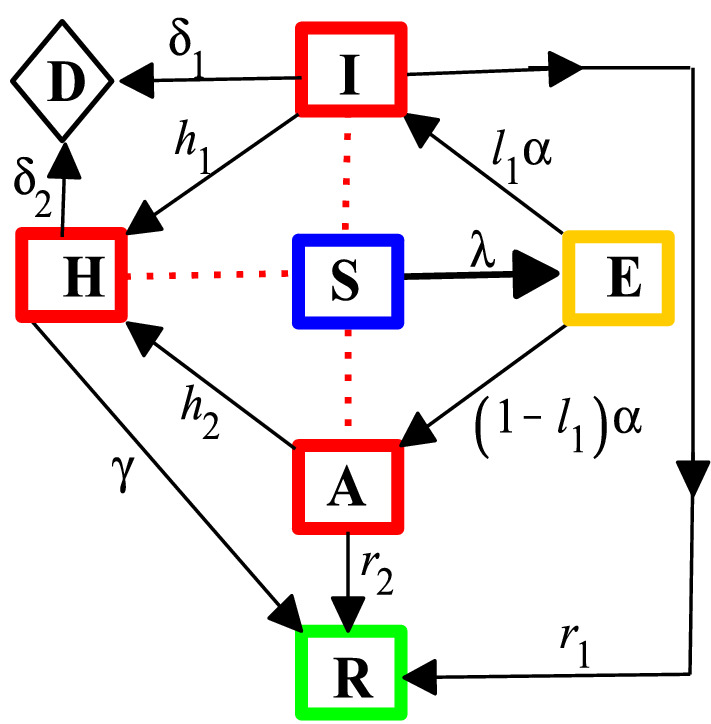
A flowchart of COVID-19 model with $\lambda =\beta S(I+{\epsilon }_{1}A+{\epsilon }_{2}H)/N-D$

Table 1.

The parameters of the COVID-19 model (1)

Parameter	Description
$\beta$	Effective transmission coefficient
${\epsilon }_1$	Modification parameter for a reduced transmission from asymptomatic humans
${\epsilon }_2$	Modification parameter for a more reduced transmission from hospitalized class
$\alpha$	Rate of disease progression from exposed class
$l_1$	Proportion of exposed with symptoms after the incubation period
$1-l_1$	Proportion of exposed without symptoms after the incubation period
$h_1$	Hospitalization rate for symptomatic class
$h_2$	Hospitalization rate for asymptomatic class after confirmation
$r_1$	Recovery rate for symptomatic class
$r_2$	Recovery rate for asymptomatic class
$\gamma$	Recovery rate for hospitalized class
${\delta }_1$	Disease-induced mortality rate for symptomatic class
${\delta }_2$	Disease-induced mortality rate for hospitalized class

Theoretical analysis of the model

It should be mentioned that the parameters of the formulated model (1) are non-negative since the model describes disease outbreak in human population. Therefore, it is suffices to state that solutions of the model (1) are non-negative.

Basic reproduction number

The potential spread of disease outbreak in a population can be determined by finding an epidemiological threshold known as the basic reproduction number. In the context of the novel coronavirus, the basic reproduction number, denoted by ${\mathfrak{R}}_0$, can be defined as the average number of secondary cases produced by one COVID-19 infected person during the course of infectiousness in a wholly susceptible population. To obtain ${\mathfrak{R}}_0$ for the COVID-19 model (1), the next generation operator technique is employed following the notations in [22]. Matrices F and V evaluated at the disease-free equilibrium (N, 0, 0, 0, 0, 0, 0) are given, respectively, by

$$\begin{array}{c}\hfill F=\left(\begin{array}{cccc}0& \beta & \beta {\epsilon }_1& \beta {\epsilon }_2\\ 0& 0& 0& 0\\ 0& 0& 0& 0\\ 0& 0& 0& 0\end{array}\right)\end{array}$$

and

$$\begin{array}{c}\hfill V=\left(\begin{array}{cccc}\alpha & 0& 0& 0\\ -l_1\alpha & h_1+r_1+{\delta }_1& 0& 0\\ -(1-l_1)\alpha & 0& h_2+r_2& 0\\ 0& -h_1& -h_2& \gamma +{\delta }_2\end{array}\right).\end{array}$$

The spectral radius of $F{V}^{-1}$, given by ${\mathfrak{R}}_0=\rho (F{V}^{-1})$, is obtained as

$$\begin{array}{c}\hfill {\mathfrak{R}}_0=\frac{\beta l_1}{k_1}+\frac{\beta {\epsilon }_1(1-l_1)}{k_2}+\frac{\beta {\epsilon }_2(l_1{h}_1{k}_2+(1-l_1)h_2{k}_1)}{k_1{k}_2{k}_3},\end{array}$$ 2

where, $k_1=h_1+r_1+{\delta }_1$, $k_2=h_2+r_2$ and $k_3=\gamma +{\delta }_2$.

Thus, the following local stability result is claimed in the sense of [22].

Theorem 1

The disease-free equilibrium (DFE) of the COVID-19 model (1) is locally asymptotically stable if the basic reproduction number, ${\mathfrak{R}}_0<1$, and unstable if ${\mathfrak{R}}_0>1$.

The implication of Theorem 1 from epidemiological viewpoint is that a small number of infected individuals present in a population will not cause an outbreak as long as ${\mathfrak{R}}_0<1$. It must be emphasized that this result depends on the initial sizes of infected individuals in the population. Hence, to rule out this dependency, a global stability result becomes necessary.

Global asymptotic stability of DFE

The global asymptotic stability of the COVID-19 free equilibrium, given by (N, 0, 0, 0, 0, 0, 0), is explored as follows.

Theorem 2

The disease-free equilibrium (DFE) of the COVID-19 model (1) is globally asymptotically stable if ${\mathfrak{R}}_0\le 1$.

Proof

The following continuously differentiable and positive definite linear Lyapunov function is carefully constructed for the COVID-19 model (1) (see, e.g., [23, 24]).

$$\begin{array}{c}\hfill \mathfrak{F}=f_{1}E+f_{2}I+f_{3}A+f_{4}H,\end{array}$$ 3

where, $f_1=[l_1{k}_2{k}_3+{\epsilon }_1(1-l_1)k_1{k}_3+{\epsilon }_2(l_1{h}_1{k}_2+(1-l_1)h_2{k}_1)]/k_1{k}_2{k}_3$, $f_2=[k_3+{\epsilon }_2{h}_1]/k_1{k}_3$, $f_3=[{\epsilon }_1{k}_3+{\epsilon }_2{h}_2]/k_2{k}_3$ and $f_4={\epsilon }_2/k_3$.

The time derivative of (3) along the solution path of the COVID-19 model (1) is given by

$$\begin{array}{cc}\hfill \dot{\mathfrak{F}}=& f_1\dot{E}+f_2\dot{I}+f_3\dot{A}+f_4\dot{H},\hfill \\ \hfill =& f_1\left(\frac{\beta S(I+{\epsilon }_{1}A+{\epsilon }_{2}H)}{N-D},-,\alpha ,E\right)+f_2(l_1\alpha E-k_{1}I)+f_3((1-l_1)\alpha E-k_{2}A)\hfill \\ \hfill & +f_4(h_{1}I+h_{2}A-k_{3}H),\hfill \\ \hfill =& f_1\left(\frac{\beta S(I+{\epsilon }_{1}A+{\epsilon }_{2}H)}{N-D}\right)-I-{\epsilon }_{1}A-{\epsilon }_{2}H,\hfill \\ \hfill \le & f_1\beta (I+{\epsilon }_{1}A+{\epsilon }_{2}H)-(I+{\epsilon }_{1}A+{\epsilon }_{2}H);(\text{since}S\le N-D),\hfill \\ \hfill =& (I+{\epsilon }_{1}A+{\epsilon }_{2}H)(f_1\beta -1),\hfill \\ \hfill =& (I+{\epsilon }_{1}A+{\epsilon }_{2}H)\left(\frac{\beta l_1}{k_1},+,\frac{\beta {\epsilon }_1(1-l_1)}{k_2},+,\frac{\beta {\epsilon }_2(l_1{h}_1{k}_2+(1-l_1)h_2{k}_1)}{k_1{k}_2{k}_3},-,1\right),\hfill \\ \hfill =& (I+{\epsilon }_{1}A+{\epsilon }_{2}H)({\mathfrak{R}}_0-1).\hfill \end{array}$$ 4

It follows that $\dot{\mathfrak{F}}\le 0$ if ${\mathfrak{R}}_0<1$ with equality, $\dot{\mathfrak{F}}=0$, if and only if $E=0$, $I=0$, $A=0$ and $H=0$. Therefore, it can be concluded from the LaSalle’s Invariance Principle [25] that the DFE is globally asymptotically stable whenever ${\mathfrak{R}}_0\le 1$. $\square$

The implication of Theorem 2 from the epidemiological viewpoint is that COVID-19 can be effectively controlled in the population if ${\mathfrak{R}}_0<1$ regardless of the initial sizes of the infected individuals. This theoretical result will be graphically illustrated later.

Parameter estimation and model fitting

This section is devoted to the estimation of parameters of the COVID-19 model (1) based on the reported data of cases in Nigeria [8]. In particular, the formulated model is parameterized to assess the burden of COVID-19 in terms of the number of individuals currently infected (active cases) in Nigeria. In this study, the values for parameters such as effective transmission coefficient ($\beta$), modification parameter (${\epsilon }_2$), and hospitalization rates ($h_1$ and $h_2$) are estimated, while the values of other parameters are chosen from the well-established literature as appeared in Table 2. The estimation of parameters is carried out using the least squares method implemented in Excel Solver [26] with a view to minimizing summation of squared errors given by $\sum {(Y(t,p)-X_{\mathit{real}})}^2$ subject to the COVID-19 model (1), where $X_{\mathit{real}}$ is the real reported data, and Y(t, p) represents the solution of the model corresponding to the number of active cases over time t with the set of estimated parameters, denoted by p.

Table 2.

Values of parameters and initial conditions

Parameter	Range	Value	Source
$\beta$	0–1	0.38974	Fitted
${\epsilon }_1$		0.5 ${\text{day}}^{-1}$	[10]
${\epsilon }_2$	0–1	0.24278	Fitted
$\alpha$		$\frac{1}{5.2}{\text{day}}^{-1}$	[29]
$l_1$	0–1	0.5	[10]
$h_1$	0.2–0.5	0.33604 ${\text{day}}^{-1}$	Fitted
$h_2$	0.1–0.25	0.19466 ${\text{day}}^{-1}$	Fitted
$r_1=r_2$	0.0333–0.3333	$\frac{1}{7}{\text{day}}^{-1}$	[11, 30]
$\gamma$	0.0333–0.3333	$\frac{1}{15}{\text{day}}^{-1}$	[10, 15]
${\delta }_1={\delta }_2$	0.001–0.1	0.015 ${\text{day}}^{-1}$	[16, 31]

Moreover, initial conditions for the exposed humans, symptomatic and asymptomatic infectious individuals are estimated to account for the possibility that the actual number of cases is most likely much higher than reported in Nigeria as in other parts of the world, due to limited testing and the possible presence of COVID-19 infected individuals with no symptoms [27]. In order to accommodate the foregoing possibility, the estimations of parameters and initial conditions for the model fitting are allowed to commence from March 10, 2020, exactly a day after the second COVID-19 confirmed case was reported by NCDC [8], so that $H(0)=2$. Keeping in mind that the total population of Nigeria is estimated at $N=200$ million people [28], and that no report of recovery and deaths due to the disease was made as at March 10, 2020 (i.e., $R(0)=D(0)=0$), then it is easy to determine the initial susceptible population as $S(0)=N-(E(0)+A(0)+I(0)+H(0)+R(0)+D(0))$.

The model is fitted to the real data along with the following initial conditions: $E(0)=880$, $A(0)=330$, $I(0)=190$, so that $S(0)=199,998,600$. The model fitting with reported active cases is depicted in Fig. 2. Consequently, the value of the basic reproduction number using the parameter values in Table 2 is ${\mathfrak{R}}_0=1.412$, which still exceeds the novel coronavirus pandemic threshold of one.

Fig. 2.

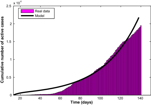
Fitting of the COVID-19 model (1) with the available cumulative number of active cases from March 10 to July 15, 2020

Sensitivity of the model to parameters

It is important to explore how sensitive the COVID-19 model (1) is to changes in each of its parameters in order to suggest intervention strategies that will help in bringing down the infection trajectory. In other words, carrying out sensitivity analysis will help in providing insights into what should be done or avoided to prevent the outbreak of the novel coronavirus [32]. Thus, as defined in [33], a relative change in the basic reproduction number, ${\mathfrak{R}}_0$, when each parameter changes is measured using the following

$$\begin{array}{c}\hfill {\mathrm{{\rm Y}}}_p^{{\mathfrak{R}}_0}=\frac{\partial {\mathfrak{R}}_0}{\partial p}\times \frac{p}{{\mathfrak{R}}_0},\end{array}$$

where, ${\mathrm{{\rm Y}}}_p^{{\mathfrak{R}}_0}$ is the sensitivity index of a differentiable ${\mathfrak{R}}_0$ with respect to any parameter, p. Consequently, the sensitivity indexes for the model (1) are graphically shown in Fig. 3. It can be observed that of all the positive indices, the effective transmission coefficient, $\beta$, is the highest, and therefore the most sensitive parameter. This means that an increase (or a decrease) of the value of $\beta$ will increase (or decrease) ${\mathfrak{R}}_0$ by 100%. However, of all the negative indices shown in Fig. 3, the recovery rate for the hospitalized class (active cases), denoted by $\gamma$, is the most sensitive parameter. This means that an increase (or a decrease) of the value of $\gamma$ will decrease (or increase) ${\mathfrak{R}}_0$ by 42.1%.

Fig. 3.

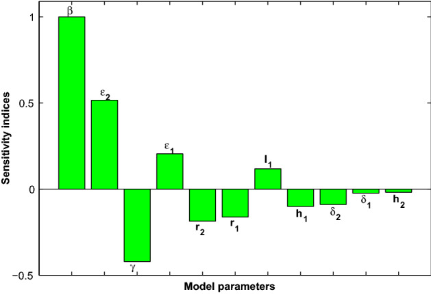
COVID-19 model sensitivities to its associated parameters

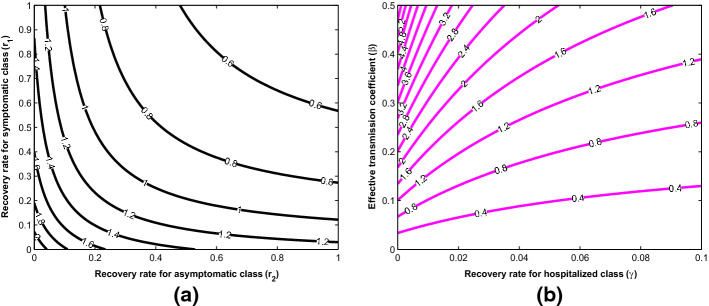
In addition, contour plots of ${\mathfrak{R}}_0$ as a function of other parameters are shown in Fig. 4 to demonstrate how changes in these parameters affect the basic reproduction number, ${\mathfrak{R}}_0$. Figure 4a shows a decrease in ${\mathfrak{R}}_0$ with increasing recovery rates for both symptomatic and asymptomatic individuals. This spontaneous recovery from infection is due to the body’s innate immune response which is capable of inhibiting virus replication, promoting virus clearance, and triggering a prolonged adaptive immune response against reinfection [34]. Moreover, it can be confirmed, as shown in Fig. 4b, that the basic reproduction number can be brought lower than the threshold of one if efforts are geared towards lowering the transmission rate while simultaneously improving on the management of active cases.

Fig. 4.

2-D contour plots of the basic reproduction number ${\mathfrak{R}}_0$

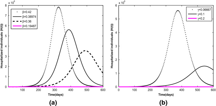
In Fig. 5a, the effects of effective transmission coefficient at different values are illustrated. It is projected that the cumulative number of active cases in Nigeria, given the current infection trajectory with $\beta =0.38974$, may get up to $5\times {10}^6$ (equivalently, 2.5% of the total estimated population) unless drastic measures are taken to bring the basic reproduction number below one. As shown in Fig. 5b, the cumulative number of active cases reduces with increasing value of recovery rate for hospitalized individuals from $\gamma =1/15{\text{day}}^{-1}$ to $1/5{\text{day}}^{-1}$. In particular, if it takes 5 days or less to effectively manage infected individuals, the risk of infection transmission from the hospitalized class will reduce significantly. This indicates that the longer it takes to effectively manage COVID-19 patient, the heavier the burden of the disease on the healthcare facility and the population at large.

Fig. 5.

Projections with varying effects of parameters: a Effective transmission coefficient at values of $\beta =[0.42({\mathfrak{R}}_0=1.521>1),0.38974({\mathfrak{R}}_0=1.412>1),0.36({\mathfrak{R}}_0=1.304>1)\text{and}0.19487({\mathfrak{R}}_0=0.706<1)]$. b Recovery rate for hospitalized individuals at values of $\gamma =[0.06667({\mathfrak{R}}_0=1.412>1),0.1({\mathfrak{R}}_0=1.2>1),\text{and}0.2({\mathfrak{R}}_0=0.959<1)]$

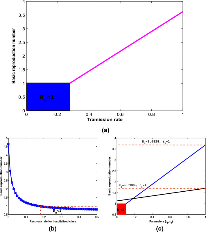
More explicitly, Fig. 6 reveals how the potential spread of the novel coronavirus in the population is affected by the model parameters in order to influence effective policies that can guide against the burden of the disease transmission. The blue rectangular box in Fig. 6a indicates a safe region where the effective transmission coefficient, $\beta$, is below a value of 0.27613, so that the key epidemiological threshold, ${\mathfrak{R}}_0$, is less than one. Above this region, the basic reproduction number which determines the spread potential of the disease increases as the rate of transmission increases through effective contact between susceptible and infectious individuals in the population. Hence, to stay in the safe region, measures such as strict social distancing and maintenance of good personal hygiene are strongly advised. This result is consistent with previous findings in the literature [9, 11, 13, 15, 17]. Furthermore, the potential spread of the diseases decreases with increase in the recovery rate as shown in Fig. 6b. The safe region of ${\mathfrak{R}}_0<1$ in this case is attained at recovery rate above the value of 0.1727. Hence, given the high infectiousness of the novel coronavirus disease, treatment regime which ensures recovery within a short period of 5 days is strongly advised. In Fig. 6c, the effects of the modification parameters, ${\epsilon }_1$ and ${\epsilon }_2$, respectively for virus transmission from asymptomatic (black solid line) and hospitalized (blue solid line) individuals on the basic reproduction number are shown. The red rectangular box is the safe region where ${\epsilon }_2$ is below a value of 0.1. Above this value, ${\mathfrak{R}}_0$ will increase up to 3.6828 which may lead to a more serious pandemic situation. Hence, strict usage of personal protective equipment when attending to the hospitalized COVID-19 individuals is strongly advised to avoid further spread of the disease.

Fig. 6.

Relationship between COVID-19 epidemiological threshold and parameters

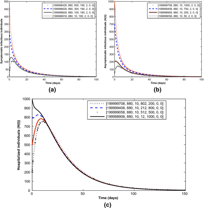
To validate the global stability result (Theorem 2), Fig. 7 illustrates the convergence to the COVID-19-free equilibrium irrespective of the initial sizes of the infectious individuals in the population.

Fig. 7.

Convergence of solution trajectories for a symptomatic humans, b asymptomatic humans and c hospitalized humans at different initial sizes in line with Theorem 2. Parameter values used are as given in Table 2 except for $\beta =0.19487$ and $\epsilon =0.12$, so that ${\mathfrak{R}}_0=0.522<1$

Optimal control model and analysis

In the light of the sensitivity analysis result, optimal control theory is applied to the COVID-19 model (1), as applied to other infectious diseases models (e.g., [33, 35–39]) in order to mitigate the spread of COVID-19 in the population optimally. This is done by introducing two time-dependent control variables $u_1(t)$ and $u_2(t)$, which are described in details as follows.

• (i)$u_1(t)$ denotes the preventive strategy targeted at inhibiting the virus transmission from symptomatic, asymptomatic and hospitalized humans. This can be achieved through public heath advocacy for social distancing, good personal hygiene, wearing face masks in public places, and provision of protective gear for healthcare workers. Noting that $u_1(t)=1$ implies the strategy is effective for protection against infection, while $u_1(t)=0$ implies strategy failure.
• (ii)$u_2(t)$ represents control variable to step up the management of hospitalized individuals with a view to ensuring prompt recovery and preventing deaths due to complications. This can be achieved through prompt provision of supplemental oxygen or mechanical ventilation for hospitalized individuals with severe COVID-19. If $u_2(t)=1$, then the control is effective in managing the disease, while $u_2(t)=0$ means the absence of control.

Consequently, the optimal control model with the two aforementioned time-dependent variables is given by the following differential equations

$$\begin{array}{c}\hfill \begin{array}{cc}\hfill {\displaystyle \frac{\mathit{dS}}{\mathit{dt}}}& =-(1-u_1(t)){\displaystyle \frac{\beta S(I+{\epsilon }_{1}A+{\epsilon }_{2}H)}{N-D}}\hfill \\ \hfill {\displaystyle \frac{\mathit{dE}}{\mathit{dt}}}& =(1-u_1(t)){\displaystyle \frac{\beta S(I+{\epsilon }_{1}A+{\epsilon }_{2}H)}{N-D}}-\alpha E\hfill \\ \hfill {\displaystyle \frac{\mathit{dI}}{\mathit{dt}}}& =l_1\alpha E-(h_1+r_1+{\delta }_1)I\hfill \\ \hfill {\displaystyle \frac{\mathit{dA}}{\mathit{dt}}}& =(1-l_1)\alpha E-(h_2+r_2)A\hfill \\ \hfill {\displaystyle \frac{\mathit{dH}}{\mathit{dt}}}& =h_{1}I+h_{2}A-(\gamma +u_2(t)+{\delta }_2)H\hfill \\ \hfill {\displaystyle \frac{\mathit{dR}}{\mathit{dt}}}& =r_{1}I+r_{2}A+(\gamma +u_2(t))H\hfill \\ \hfill {\displaystyle \frac{\mathit{dD}}{\mathit{dt}}}& ={\delta }_{1}I+{\delta }_{2}H.\hfill \end{array}\end{array}$$ 5

The aim of introducing the two control variables is to seek the optimal solution required to minimize the numbers of symptomatic, asymptomatic and hospitalized individuals responsible for spreading the novel coronavirus in the population at minimum cost. Hence, the objective functional for this control problem is given by

$$\begin{array}{c}\hfill \begin{array}{c}{\displaystyle \mathfrak{J}(u_1,u_2)={min}_{0\le u_1,u_2\le 1}{\int }_0^{T_f}\left(w_1,I,+,w_2,A,+,w_3,H,+,\frac{1}{2},[w_4{u}_1^2(t)+w_5{u}_2^2(t)]\right)dt,}\hfill \end{array}\end{array}$$ 6

where, constants $w_i,i=1,2,...,5$ are positive weights required to balance the corresponding terms in the objective functional. Following other literature on COVID-19 control problems [9, 16, 17, 40, 41], quadratic costs on the controls are chosen, where $1/2w_4{u}_1^2(t)$ is the total cost of implementing the preventive measure, and $1/2w_5{u}_2^2(t)$ is the total cost of managing active cases over the time interval $[0,T_f]$.

Precisely, the optimal control double $u^{\ast }=(u_1^{\ast },u_2^{\ast })$ is sought such that

$$\begin{array}{c}\hfill \mathfrak{J}(u_1^{\ast },u_2^{\ast })=min\left\{\mathfrak{J},(u_1,u_2),:,u_1,,,u_2,\in ,\mathcal{U}\right\},\end{array}$$ 7

where, $\mathcal{U}$ is the non-empty control set defined by

$\mathcal{U}=\left\{(u_1,u_2),:,(u_1(t),u_2(t)),,\text{are measurable with},,0,\le ,u_1,,,u_2,\le ,1,,\text{for},,t,\in ,[0,T_f]\right\}$. Thus, to determine the necessary conditions that the optimal control double ($u_1^{\ast },u_2^{\ast }$) must satisfy, Pontryagin’s maximum principle [42], which transforms the control problem (7) subject to the model (5) into a problem of minimizing pointwise a Hamiltonian $\mathcal{H}$, is used. This Hamiltonian is given by

$$\begin{array}{cc}\hfill \mathcal{H}=& w_{1}I+w_{2}A+w_{3}H+\frac{1}{2}[w_4{u}_1^2(t)+w_5{u}_2^2(t)]\hfill \\ \hfill & +{\lambda }_1\left[-,(1-u_1(t)),{\displaystyle \frac{\beta S(I+{\epsilon }_{1}A+{\epsilon }_{2}H)}{N-D}}\right]\hfill \\ \hfill & +{\lambda }_2\left[(1-u_1(t)),{\displaystyle \frac{\beta S(I+{\epsilon }_{1}A+{\epsilon }_{2}H)}{N-D}},-,\alpha ,E\right]\hfill \\ \hfill & +{\lambda }_3[l_1\alpha E-(h_1+r_1+{\delta }_1)I]+{\lambda }_4[(1-l_1)\alpha E-(h_2+r_2)A]\hfill \\ \hfill & +{\lambda }_5[h_{1}I+h_{2}A-(\gamma +u_2(t)+{\delta }_2)H]\hfill \\ \hfill & +{\lambda }_6[r_{1}I+r_{2}A+(\gamma +u_2(t))H]+{\lambda }_7[{\delta }_{1}I+{\delta }_{2}H],\hfill \end{array}$$ 8

where, ${\lambda }_i$, $i=1,2,3,...,7$, represent the adjoint variables associated with the state variables of the model (5). The standard existence result for minimizing control problem as appeared in [43, 44] is adapted as follows.

Theorem 3

Given that $(u_1^{\ast },u_2^{\ast })$ minimizes the objective functional (6) subject to the corresponding state system (5), then the adjoint variables ${\lambda }_i$, $i=1,2,3,...,7$, satisfy the following system

$$\begin{array}{c}\hfill \begin{array}{cc}\hfill \frac{d{\lambda }_1}{\mathit{dt}}& ={\displaystyle \frac{\beta (1-u_1(t))(I+{\epsilon }_{1}A+{\epsilon }_{2}H)[{\lambda }_2-{\lambda }_1]}{N-D}}\hfill \\ \hfill \frac{d{\lambda }_2}{\mathit{dt}}& =\alpha ({\lambda }_2-l_1{\lambda }_3-(1-l_1){\lambda }_4)\hfill \\ \hfill \frac{d{\lambda }_3}{\mathit{dt}}& ={\displaystyle \frac{\beta S(1-u_1(t))[{\lambda }_2-{\lambda }_1]}{N-D}}+{\delta }_1({\lambda }_3-{\lambda }_7)+h_1({\lambda }_3-{\lambda }_5)+r_1({\lambda }_3-{\lambda }_6)-w_1\hfill \\ \hfill \frac{d{\lambda }_4}{\mathit{dt}}& ={\displaystyle \frac{{\epsilon }_1\beta S(1-u_1(t))[{\lambda }_2-{\lambda }_1]}{N-D}}+h_2({\lambda }_4-{\lambda }_5)+r_2({\lambda }_4-{\lambda }_6)-w_2\hfill \\ \hfill \frac{d{\lambda }_5}{\mathit{dt}}& ={\displaystyle \frac{{\epsilon }_2\beta S(1-u_1(t))[{\lambda }_2-{\lambda }_1]}{N-D}}+{\delta }_2({\lambda }_5-{\lambda }_7)+(\gamma +u_2(t))({\lambda }_5-{\lambda }_6)-w_3\hfill \\ \hfill \frac{d{\lambda }_6}{\mathit{dt}}& =0\hfill \\ \hfill \frac{d{\lambda }_7}{\mathit{dt}}& ={\displaystyle \frac{\beta (1-u_1(t))S(I+{\epsilon }_{1}A+{\epsilon }_{2}H)[{\lambda }_1-{\lambda }_2]}{{(N-D)}^2}}\hfill \end{array}\end{array}$$ 9

with the terminal (transversality) conditions

$$\begin{array}{c}\hfill \begin{array}{c}{\lambda }_i(T_f)=0,i=1,2,3,...,7.\hfill \end{array}\end{array}$$ 10

Further, the optimal control double $(u_1^{\ast },u_2^{\ast })$ is given as follows

$$\begin{array}{cc}\hfill u_1^{\ast }=& max\left\{0,,,min,\left\{1,,,{\displaystyle \frac{\beta S(I+{\epsilon }_{1}A+{\epsilon }_{2}H)[{\lambda }_2-{\lambda }_1]}{w_4(N-D)}}\right\}\right\},\hfill \\ \hfill u_2^{\ast }=& max\left\{0,,,min,\left\{1,,,{\displaystyle \frac{H[{\lambda }_5-{\lambda }_6]}{w_5}}\right\}\right\}.\hfill \end{array}$$ 11

Proof

The existence of the optimal control double ($u_1,u_2$) is based on the a priori boundedness of the state variables of model (5), convexity and boundedness of the Langragian of the control problem. The system of ordinary differential equations (9) governing the adjoint variables is derived by differentiating the Hamiltonian $\mathcal{H}$. Further, the control characterizations in (11) are derived by solving, on the interior of the control set $\mathcal{U}$, the partial differentials of the Hamiltonian $\mathcal{H}$ with respect to each of the controls $u_1$ and $u_2$. Hence, by standard arguments involving control bounds, it follows that

$$\begin{array}{c}\hfill u_1^{\ast }=\left\{\begin{array}{cc}0\hfill & \text{if}{\tau }_1^{\ast }\le 0,\hfill \\ {\tau }_1^{\ast }\hfill & \text{if}0<{\tau }_1^{\ast }<1,\hfill \\ 1\hfill & \text{if}{\tau }_1^{\ast }\ge 1,\hfill \end{array}\right)\end{array}$$

and

$$\begin{array}{c}\hfill u_2^{\ast }=\left\{\begin{array}{cc}0\hfill & \text{if}{\tau }_2^{\ast }\le 0,\hfill \\ {\tau }_2^{\ast }\hfill & \text{if}0<{\tau }_2^{\ast }<1,\hfill \\ 1\hfill & \text{if}{\tau }_2^{\ast }\ge 1,\hfill \end{array}\right)\end{array}$$

where,

$$\begin{array}{c}\hfill {\tau }_1^{\ast }={\displaystyle \frac{\beta S(I+{\epsilon }_{1}A+{\epsilon }_{2}H)[{\lambda }_2-{\lambda }_1]}{w_4(N-D)}}\end{array}$$

and

$$\begin{array}{c}\hfill {\tau }_2^{\ast }={\displaystyle \frac{H[{\lambda }_5-{\lambda }_6]}{w_5}}.\end{array}$$

This ends the proof. $\square$

Simulations of the control probem

Forward and backward Runge-Kutta method of order four implemented in MATLAB is used to solve the resulting optimality system which consists of systems (5) and (9) with the characterizations (11) within the time interval of [0, 100] days. The weight constants used for balancing the terms in the objective functional (6) are chosen to ensure that no term dominates the other. Thus, equal weight constant for minimizing the infectious classes is chosen, so that $w_1=w_2=w_3=1$. On the other hand, the weight constants for measuring efforts or costs required to implement the controls are comparatively different. This results in values for $w_4=50$ and $w_5=100$. Details of the numerical procedure for simulating the obtained optimality system are contained in [45].

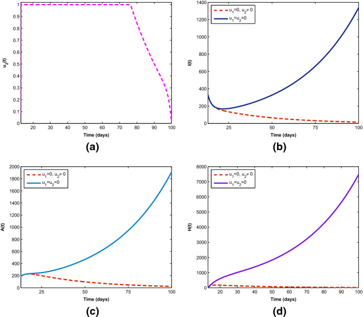
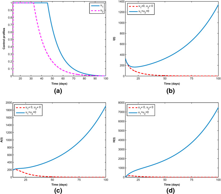
Figure 8 demonstrates how single preventive measure, $u_1(t)$, affects the spread of the novel coronavirus in the population. As shown in Fig. 8a, to minimize the objective functional (6), the optimal control $u_1(t)$ is maintained at maximum level of 100% for about 93 days before relaxing to the minimum in final time. As expected, the sizes of COVID-19 infectious individuals are reduced when control is in place. Further, in Fig. 9a, b, the effects of single management control, $u_2(t)$, are shown in minimizing the number of virus infection in the population, but not as much as when only preventive strategy is applied. More importantly, Fig. 10 shows the significance of combining the two optimal controls in bringing down the total number of infectious humans to zero. It is observed that optimal solution is attained when preventive measure is strictly adhered to at maximum level of 100% for 45 days, while the management control of the hospitalized individuals is at maximum level of 100% for 32 days. It can be seen that combination of the two controls is significantly more effective in curbing the spread of the virus than when each control is singly applied.

Fig. 8.

Control profile ($u_1(t)$) and its effects on the COVID-19 dynamics

Fig. 9.

Control profile ($u_2(t)$) and its effects on the COVID-19 dynamics

Fig. 10.

Combined effects of optimal controls $u_1(t)$, $u_2(t)$ on the COVID-19 dynamics

Cost-effectiveness analysis

It is important to determine the most cost-effective optimal control measure among the single and combined implementation of the two given control measures in order to optimally mitigate the spread of COVID-19 at the lowest cost possible. Hence, cost-effectiveness analysis is explored using the incremental cost effectiveness ratio (ICER) [9, 24, 46–48]. To avoid dissipation of available limited resources, ICER is used to compare any two competing measures for controlling the spread of disease or related problems. The ICER formula is given by

$$\begin{array}{c}\hfill \text{ICER}=\frac{\text{Change in total costs between control measures}}{\text{Change in total number of infection averted by control measures}}.\end{array}$$ 12

The total cost for each of the single implementation and combined effort of the control measures is derivable from the objective functional 6, while the infection averted is obtained by calculating the difference between infectious individuals without and with control measures. Let $C_1$, $C_2$ and $C_{12}$ represent single implementation of the preventive measure $u_1(t)$, single implementation of the management control $u_2(t)$ and combined effort of the two measures, respectively. In what follows, Table 3 summarizes the ICER for each and combination of the control variables $u_1(t)$ and $u_2(t)$ in an increasing order of the total infection averted.

Table 3.

ICER in the order of COVID-19 cases averted by control measures

Control measures	Total infection averted	Total costs	ICER
$C_1$	$3.5062\times {10}^6$	$4.7351\times {10}^4$	0.0135
$C_2$	$3.7311\times {10}^6$	$8.2886\times {10}^4$	0.1580
$C_{12}$	$3.8848\times {10}^6$	$5.0064\times {10}^4$	$-0.2136$

Using (12), the ICER for $C_1$, $C_2$ and $C_{12}$ shown in Table 3 are calculated, respectively, as follows.

$$\begin{array}{cc}\hfill \text{ICER}(C_1)=& \frac{4.7351\times {10}^4}{3.5062\times {10}^6}=0.0135,\hfill \\ \hfill \text{ICER}(C_2)=& \frac{(8.2886-4.7351)\times {10}^4}{(3.7311-3.5062)\times {10}^6}=0.1580,\hfill \\ \hfill \text{ICER}(C_{12})=& \frac{(5.0064-8.2886)\times {10}^4}{(3.8848-3.7311)\times {10}^6}=-0.2136.\hfill \end{array}$$

Comparing $C_1$ and $C_2$, it is seen that ICER($C_1$) is less than ICER($C_2$). This means that $C_2$ is more costly and less effective than $C_1$. In other words, $C_1$ dominates $C_2$. Thus, single implementation of management control is removed from the list. As a consequence, $C_1$ and $C_{12}$ are assessed in Table 4 using similar procedure.

Table 4.

Comparison between $C_1$ and $C_{12}$

Control measures	Total infection averted	Total costs	ICER
$C_1$	$3.5062\times {10}^6$	$4.7351\times {10}^4$	0.0135
$C_{12}$	$3.8848\times {10}^6$	$5.0064\times {10}^4$	0.0072

It is revealed in Table 4 that $C_1$ is dominated by $C_{12}$ since ICER($C_1$) is greater than ICER($C_{12}$). This implies that $C_{12}$ is less costly and more effective than $C_1$. Hence, single implementation of preventive measure is excluded from the list. This shows that combined effort of the two control measures is the most cost-effective intervention capable of diminishing the burden of the novel coronavirus optimally in the host population.

Conclusion

This study presented a mathematical analysis of transmission dynamics of the novel coronavirus (COVID-19) pandemic with a view to providing further insights into the disease transmission, and to explore possible prevention and control measures capable of curbing the rising tide of the disease spread in the population. A deterministic mathematical model was formulated by subdividing the host population into susceptible, exposed, symptomatic infectious, asymptomatic infectious, hospitalized, recovered and dead classes. The nonlinear model has been developed by considering transmission routes from symptomatic infectious humans, asymptomatic infectious humans and hospitalized individuals. The theoretical analysis carried out, based on Lyapunov stability, showed that the model has a globally asymptotically stable disease-free equilibrium if the basic reproduction number of the novel coronavirus transmission is less than one. This is an indication that COVID-19 outbreak can be effectively controlled in the population irrespective of the number of the infectious individuals initially introduced into the completely susceptible population.

In particular, the formulated model was fitted to the reported data of cumulative number of hospitalized individuals (active cases) due to COVID-19 in Nigeria, and estimates for parameters such as, effective transmission coefficients ($\beta$), modification parameter for the transmission of virus infection from active cases (${\epsilon }_2$), hospitalization rates for both symptomatic and asymptomatic individuals ($h_1$ and $h_2$) were determined using the least squares method. Sensitivity analysis of the fitted model was performed to find the parameters that drive the spread of the virus infection mostly in the population. It was revealed that $\beta$ is the most sensitive parameter, followed by ${\epsilon }_2$ and the recovery rate for active cases denoted by $\gamma$. In addition, given the high infectiousness of the novel coronavirus disease, safe regions where virus infection dies out at certain threshold values of the model parameters were derived in order to facilitate and strengthen formulation of effective policies that can help to avoid a more serious pandemic situation. Further insights into the projection of the disease transmission indicated that the cumulative number of active cases in Nigeria, given the current infection trajectory, may get up to 2.5% of the total estimated population of 200 million, unless drastic measures are taken to bring the basic reproduction number below one. It was shown by simulations that the basic reproduction number can be brought to a value less than one in Nigeria, if the current effective transmission rate of the disease can be reduced by 50%.

Moreover, the model was extended to include time-dependent optimal control variables (preventive and management measures) to examine their impacts in minimizing the burden of COVID-19 in the population using Pontryagin’s maximum principle. The optimal preventive measure was shown to be better than management control in reducing the burden of the disease, but the combined effort of the two controls has significant effect in reducing the number of infectious individuals in the population. This result was further supported by carrying out the cost-effectiveness analysis, and it was therefore established that the combined implementation of the two control measures is the most cost-effective when compared with the single implementation of each control measure.

In view of the above, it can be concluded that flattening of the novel coronavirus infection curve largely depends on two key parameters, namely effective transmission coefficient and recovery rate. Efforts geared toward lowering the transmission rate and improving on the treatment regime for quick recovery of cases are required to ensure virus-free region and effectively overcome the spread of the novel coronavirus in the host population. To achieve this optimally, it is recommended that adherence to the combination of preventive and management control measures should be strict. These measures include continued public advocacy for social distancing, good personal hygiene, wearing face masks in public places, provision of protective gear for healthcare workers caring for people with COVID-19 infection. If strict adherence is practiced, transmission routes from symptomatic, asymptomatic and hospitalized individuals will be effectively hindered, and availability of supplemental oxygen or mechanical ventilation for hospitalized individuals with severe COVID-19. In addition, given the ongoing community spread of the virus in Nigeria and almost all the countries of world, the need to scale up the testing capacity for detection and prompt treatment of asymptomatic individuals cannot be overemphasized in order to nip the transmission of the novel coronavirus in the bud. It is also pertinent to advise that healthcare facilities should not only be increased, but well equipped to accommodate the increasing spate of cases and effectively manage patients who may develop complications due the novel coronavirus infection.

Data Availability Statement

This manuscript has associated data in a data repository. [Authors’ comment: Available at Nigeria Centre for Disease Control (NCDC). https://covid19.ncdc.gov.ng/report/.]

Compliance with ethical standards

Conflict of interest

The authors declare no conflict of interest.

References

- 1.Chakraborty I, Maity P. Sci. Total Environ. 2020;728:138882. doi: 10.1016/j.scitotenv.2020.138882. [DOI] [PMC free article] [PubMed] [Google Scholar]
- 2.World Health Organization (WHO) Q&A on coronaviruses (COVID-19). https://www.who.int/emergencies/diseases/novel-coronavirus-2019/question-and-answers-hub/q-a-detail/q-a-coronaviruses (Accessed July 16 2020)
- 3.Worldometer Coronavirus worldwide graphs (2020) https://www.worldometers.info/coronavirus/worldwide-graphs/ (Accessed July 16 2020)
- 4.Nigeria Centre for Disease Control (NCDC), FAQs. https://covid19.ncdc.gov.ng/faq/ (Accessed July 12 2020)
- 5.Bai Y, Yao L, Wei T, Tian F, Jin DY, Chen L, Wang M. JAMA. 2020;323:1406. doi: 10.1001/jama.2020.2565. [DOI] [PMC free article] [PubMed] [Google Scholar]
- 6.Rothe C, Schunk M, Sothmann P, et al. New Engl. J. Med. 2020 doi: 10.1056/NEJMc2001468. [DOI] [PMC free article] [PubMed] [Google Scholar]
- 7.Zou L, Ruan F, Huang M, et al. New Engl. J. Med. 2020;382:1177. doi: 10.1056/NEJMc2001737. [DOI] [PMC free article] [PubMed] [Google Scholar]
- 8.Nigeria Centre for Disease Control (NCDC), COVID-19 Nigeria. https://covid19.ncdc.gov.ng/report/. (Accessed July 16 2020)
- 9.Asamoah JKK, Owusu MA, Jin Z, Oduro FT, Abidemi A, Gyasi EO. Chaos. Solitons. Fractals. 2020;140:110103. doi: 10.1016/j.chaos.2020.110103. [DOI] [PMC free article] [PubMed] [Google Scholar]
- 10.Chen T-M, Rui J, Wang Q-P, Zhao Z-Y, Cui J-A, Yin J. Infect. Dis. Poverty. 2020 doi: 10.1186/s40249-020-00640-3. [DOI] [PMC free article] [PubMed] [Google Scholar]
- 11.Iboi EA, Sharomi OO, Ngonghala CN, Gumel AB. Math. Biosci. Eng. 2020;17:6. doi: 10.3934/mbe.2020369. [DOI] [PubMed] [Google Scholar]
- 12.Jia J, Ding J, Liu S, et al. Electron. J. Differ. Equ. 2020;2020:23. doi: 10.1186/s13662-019-2480-y. [DOI] [Google Scholar]
- 13.Mushayabasa S, Ngarakana-Gwasira ET, Mushanyu J. Inform. Med. Unlocked. 2020;20:100387. doi: 10.1016/j.imu.2020.100387. [DOI] [PMC free article] [PubMed] [Google Scholar]
- 14.Nabi KN. Chaos. Solitons. Fractals. 2020;139:110046. doi: 10.1016/j.chaos.2020.110046. [DOI] [PMC free article] [PubMed] [Google Scholar]
- 15.Okuonghae D, Omame A. Chaos. Solitons. Fractals. 2020;139:110032. doi: 10.1016/j.chaos.2020.110032. [DOI] [PMC free article] [PubMed] [Google Scholar]
- 16.A. Srivastav, M. Ghosh, X. Li, L. Cai, Authorea. (2020). 10.22541/au.159317504.46174347
- 17.Ullah L, Khan MA. Chaos. Solitons. Fractals. 2020;139:110075. doi: 10.1016/j.chaos.2020.110075. [DOI] [PMC free article] [PubMed] [Google Scholar]
- 18.Xue L, Jing S, Miller JC, et al. Math. Biosci. 2020;326:108391. doi: 10.1016/j.mbs.2020.108391. [DOI] [PMC free article] [PubMed] [Google Scholar]
- 19.Kermack WO, McKendrick AG. Soc. Lond. Series A. 1927;115:700. [Google Scholar]
- 20.Ndairou F, Area I, Nieto JJ, Torres DFM. Chaos. Solitons. Fractals. 2020;135:109846. doi: 10.1016/j.chaos.2020.109846. [DOI] [PMC free article] [PubMed] [Google Scholar]
- 21.Punch Healthwise, https://healthwise.punchng.com/812-healthcare-workers-infected-with-covid-19-ncdc/ (Accessed July 7 2020)
- 22.van den Driessche P, Watmough J. Math. Biosci. 2002;180:29. doi: 10.1016/S0025-5564(02)00108-6. [DOI] [PubMed] [Google Scholar]
- 23.Akanni JO, Olaniyi S, Akinpelu FO. J. Appl. Math. Comput. 2020 doi: 10.1007/s12190-020-01423-7. [DOI] [Google Scholar]
- 24.Ghosh M, Olaniyi S, Obabiyi OS. Appl. Math. Comput. 2020;373:125044. doi: 10.1016/j.amc.2020.125044. [DOI] [Google Scholar]
- 25.J.P. LaSalle, The stability of dynamical systems. in Regional Conference Series in Applied Mathematics (SIAM, Philadelphia, 1976)
- 26.L. Chandrakantha, Using Excel Solver in Optimization Problems (Mathematics and Computer Science Department, New York, 2008)
- 27.Human Rights Watch, Nigeria: COVID-19 Cases on the Rise, https://www.hrw.org/news/2020/03/25/nigeria-covid-19-cases-rise# (Accessed 21 June 2020)
- 28.Trading Economics, Nigeria population, https://tradingeconomics.com/nigeria/population (Accessed July 18 2020)
- 29.Li Q, Guan X, Wu P, Wang X, Zhou L, Tong Y, et al. New Engl. J. Med. 2020 doi: 10.1056/NEJMoa2001316. [DOI] [Google Scholar]
- 30.Tang B, Wang Q, Li N, Bragazzi S, Tang Y, et al. J. Clin. Med. 2020;9:462. doi: 10.3390/jcm9020462. [DOI] [PMC free article] [PubMed] [Google Scholar]
- 31.N.M. Ferguson, D. Laydon, G. Nedjati-Gilani, N. Imai, K. Ainslie et al., Impact of non-pharmaceutical interventions (NPIs) to reduce COVID-19 mortality and healthcare demand. (Imperial College COVID-19 Response Team, London, 2020). 10.25561/77482
- 32.M.S. Islam, J.I. Ira, K.M. Kabir, M. Kamrujjaman, Preprint. (2020). 10.20944/preprints202004.0193.v2
- 33.Olaniyi S. Appl. Math. Inf. Sci. 2018;12:969. doi: 10.18576/amis/120510. [DOI] [Google Scholar]
- 34.Li G, Fan Y, Lai Y, Han T, Li Z, et al. J. Med. Virol. 2020 doi: 10.1002/jmv.25685. [DOI] [PMC free article] [PubMed] [Google Scholar]
- 35.Abidemi A, Aziz NAB. Comput. Methods Program Biomed. 2020;196:105585. doi: 10.1016/j.cmp.2020.105585. [DOI] [PubMed] [Google Scholar]
- 36.S.F. Abimbade, S. Olaniyi, O.A. Ajala, M.O. Ibrahim, Optim. Control. Appl. Meth. (2020). 10.1002/oca.2658
- 37.Okosun KO, Khan MA, Bonyah E, Ogunlade ST. Eur. Phys. J. Plus. 2017;132:363. doi: 10.1140/epjp/i2017-11625-3. [DOI] [Google Scholar]
- 38.Okosun KO. J. Biol. Syst. 2020 doi: 10.1142/S0218339020400082. [DOI] [Google Scholar]
- 39.Olaniyi S, Okosun KO, Adesanya SO, Areo EA. Open. Infect Dis. 2018;10:166. doi: 10.2174/1874279301810010166. [DOI] [Google Scholar]
- 40.Khajji B, Kada D, Balatif O, Rachik M. J. Appl. Math. Comput. 2020 doi: 10.1007/s12190-020-01354-3. [DOI] [PMC free article] [PubMed] [Google Scholar]
- 41.S.E. Moore, E. Okyere, arXiv preprint. (2020) arXiv:2004.00443v2 [q-bio.PE]
- 42.Pontryagin LS, Boltyanskii VG, Gamkrelidze RV, Mishchenko EF. The Mathematical Theory of Optimal Processes. New York: Wiley; 1962. [Google Scholar]
- 43.Fleming WH, Richel RW. Deterministic and Stochastic Optimal Control. New York: Springer; 1975. [Google Scholar]
- 44.Olaniyi S, Okosun KO, Adesanya SO, Lebelo RS. J. Biol. Dyn. 2020;14:90. doi: 10.1080/17513758.2020.1722265. [DOI] [PubMed] [Google Scholar]
- 45.Lenhart S, Workman JT. Optimal Control Applied to Biological Models. London: Chapman & Hall; 2007. [Google Scholar]
- 46.Okosun KO, Rachid O, Marcus N. BioSystems. 2013;111:83. doi: 10.1016/j.biosystems.2012.09.008. [DOI] [PubMed] [Google Scholar]
- 47.Akanni JO, Akinpelu FO, Olaniyi S, Oladipo AT, Ogunsola AW. Int. J. Dyn. Control. 2020;8:531. doi: 10.1007/s40435-019-00572-3. [DOI] [Google Scholar]
- 48.Lambura AG, Mwanga GG, Luboobi L, Kuznetsov D. Comput. Math. Meth. Med. 2020 doi: 10.1155/2020/6721919. [DOI] [PMC free article] [PubMed] [Google Scholar]
Associated Data
This section collects any data citations, data availability statements, or supplementary materials included in this article.