Evaluation of the effect of different policies in the containment of epidemic spreads for the COVID-19 case

Abstract

The paper presents a new mathematical model for the SARS-CoV-2 virus propagation, designed to include all the possible actions to prevent the spread and to help in the healing of infected people. After a discussion on the equilibrium and stability properties of the model, the effects of each different control actions on the evolution of the epidemic spread are analysed, through numerical evaluations for a more intuitive and immediate presentation, showing the consequences on the classes of the population.

Highlights

• •A new mathematical model for the spread of the SARS-CoV-2 is proposed and analysed.
• •Available control actions are considered including social and political decisions.
• •The effects on populations of containment policies and medical efforts are described.
• •The model can support choices for large scale strategies of diseases contrast.
• •Control actions can be defined according to economic, healthy and social issues.

1. Introduction

As for all dynamical systems, when dealing with epidemic spreads a mathematical model is the basis of realistic interpretation of the behaviours and of reliable forecast of the evolutions.

From the earliest contribution of [1], where the simplest and used SIR model (Susceptible, Infected and Recovered individuals) is introduced, several richer and more specific models have been proposed in last decades, developed for specific classes of infections, to better describe their propagation and to particularise the specific control actions against their spread.

One example in this context is the HIV/AIDS disease, for which no effective vaccine is known yet; the models have to classify the population into a higher number of classes and, due to the severity of the disease, the interventions must be reconsidered with respect to classical ones [2], [3], [4], [5], [6], [7].

Another important example is the measles disease [8], [9], [10], [11]; in this case the vaccination is available but the relatively high number of immuno-depressed individuals needs additional controls and then a more specific mathematical model to include them [12].

At present, the worldwide ongoing COVID-19 due to the SARS-CoV-2 virus spread [13], [14], [15], [16] presents the necessity to deal with ad hoc models able to describe the peculiar characteristics of the virus propagation as well as the specific possible intervention actions. The definition of a mathematical model to describe the phenomenon [14], to estimate its diffusivity [17], [18] and to give a realistic prediction to prepare the most suitable countermeasures [19] have represented the first contributions, but mainly referring or re-adapting known epidemic models.

Driven by specific characteristics of the COVID-19, evidenced day after day during the phenomenon analysis, ad-hoc models have been subsequently proposed. Among the long list, in [14] an earlier quite rich model is proposed, composed by 8 different classes and the model parameters are identified on the basis of the available data.

Same approach is found in [20], where the incubating, symptomatically and asymptomatically infectious compartments are considered to better describe the different phases of the infective evolution of the epidemic; similarly, in [21] the latency period is put in evidence and the analysis is performed fitting the Chinese data of the period from January 19 to March 18, 2020.

The pandemic characteristics of the disease motivate also analysis as in [16], where geographical movements are considered.

Regarding the support for predicting ability of a mathematical model, in [19] a short time forecast is provided, based on the uncertain data available and making reference to models developed for similar cases [22], [23], [24], [25].

Due to the unavailability of a vaccine, like for the AIDS, in the COVID-19 case a mathematical model to be used for control design [9], [26], [27], [28], [29], [29], [30], [31] must include all possible lines of interventions to better distribute the efforts and then, hopefully, increase the effects.

Analysis of the effects of individual isolation, like lockdown policies, as the possible control action, is performed in [32], where the idea that a qualitative analysis is more significant than a quantitative one and, consequently, all the numerical simulations are carried out on the basis of average values for the model parameters obtained by realistic assumptions.

In this paper, a mathematical model for SARS-CoV-2 diffusion, different from the ones previously presented, is introduced; differently from the other cited cases, all the known preventive and active actions that can be put in place are considered, at an organisational and decisional level as well as from a medical point of view, to contain the virus spread and its negative consequences.

This particular attention devoted to the control possibility brings, in this first analysis, to a characterisation of the effects of each control on the system behaviour, for each class considered, in view of the design of effective and sustainable controls.

The changes in the epidemic evolution are analysed through numerical evaluations for each action and for different control efforts. The actual effectiveness of each control, or any combination, is not faced here, being strongly dependent on the real or moral costs associated to the choices, as the recent policies adopted by the different Governments prove.

Despite the analysis is performed mainly from a qualitative point of view, all the numerical evaluations are made realistic since the model parameters are identified making use of the first official data available from Chinese Government for the Wuhan region. Clearly, different populations or geographical areas can be easily addressed once the specific data are used. This fact supports the generality of the model structure and the possibility to be used, adapting the numerical values, to any specific context without loss of validity of the qualitative results here shown.

In Section 2 the model is introduced and illustrated, with a particular attention to the choices for the numerical values of the parameters. In Section 3, a first validation of the model by considering real data of Wuhan is performed; this procedure is also used for tuning the model parameters assumed in the simulations. The Section keeps on with the illustration and the description, through numerical simulations performed on the basis of the proposed model, of the effects of each single different control actions. Section 4 is devoted to the validation of the proposed model making use of two different real cases of Countries which adopted different control approaches: Italy and United Kingdom. This analysis, which supports the reliability of the model, shows the actual correspondence of the epidemic behaviour to the changes in the control actions.

In Section 5 some conclusions are discussed.

2. The mathematical model

The mathematical model here adopted is an enrichment of a classical SEIR one, usually adopted to describe the dynamics of epidemic spreads in presence of a virus incubation phase (E) [33].

Making reference to the recent work [16] on the COVID-19, in this contribution two new classes are added and the possible ways of intervention are modelled in order to make available some numerical evaluations about the possible epidemic diffusion depending on the different strategies.

In Section 2.1 the model is described; the analysis of the equilibrium conditions and the stability properties are reported in Section 2.2, while the relationship between the basic reproduction number $R_0$, which defines the spread characteristics of the epidemic, and the model parameters is analytically defined and discussed in Section 2.3.

2.1. The mathematical model adopted

The mathematical model proposed is

$$\dot{S}\left(t\right)=B-\beta (1-u_2\left(t\right))S\left(t\right)I_C\left(t\right)+bnQ\left(t\right)+cn{u}_5\left(t\right)Q\left(t\right)-a{u}_1\left(t\right)S\left(t\right)-d_{S}S\left(t\right)$$ (1)

$$\dot{E}\left(t\right)=\beta (1-u_2\left(t\right))S\left(t\right)I_C\left(t\right)-a{u}_1\left(t\right)E\left(t\right)-kE\left(t\right)-d_{E}E\left(t\right)$$ (2)

$${\dot{I}}_C\left(t\right)=kE\left(t\right)-a{u}_1\left(t\right)I_C\left(t\right)-h_1{I}_C\left(t\right)-h_2{I}_C\left(t\right)-d_{I_C}{I}_C\left(t\right)$$ (3)

$${\dot{I}}_Q\left(t\right)=h_1{I}_C\left(t\right)+h_1(1-n)Q+c(1-n)u_5\left(t\right)Q\left(t\right)-\left(\gamma +\eta u_3\left(t\right)\right)I_Q\left(t\right)-d_{I_Q}(1-u_4\left(t\right))I_Q\left(t\right)$$ (4)

$$\dot{Q}\left(t\right)=a{u}_1\left(t\right)\left(S\left(t\right)+E\left(t\right)+I_C\left(t\right)\right)-bnQ\left(t\right)-h_1(1-n)Q-c{u}_5\left(t\right)Q\left(t\right)-d_{Q}Q\left(t\right)$$ (5)

$$\dot{R}\left(t\right)=h_2{I}_C\left(t\right)+\left(\gamma +\eta u_3\left(t\right)\right)I_Q\left(t\right)-d_{R}R\left(t\right)$$ (6)

where $S$ are the susceptible people, $E$ are the exposed individuals, infected but not infective, $I_C$ are the infected patients without symptoms, asymptomatic until the healing or until symptoms arise: they are infective and then responsible of the disease spread, $I_Q$ are the diagnosed infected patients, isolated and then not contagious: patients in this class are the ones that can receive medical treatment both for the infection and for secondary diseases or complications, $Q$ are the suspected infected individuals which are temporarily isolated and tested for positivity of the SARS-CoV-2, or simply quarantined for safeness reasons, $R$ are the recovered individuals, supposed to be no more infected and then not infective.

As far as the model parameters is concerned, their meaning is as follows. All the $d_{\ast }$ terms denote the death rates in each class. The term $B$ denotes the constant inflow rate of new individuals. Coefficient $\beta$ is the contact rate. Parameters $k$, $h_1$, $h_2$ and $\gamma$ denote the natural transition rates between classes: $k$ is referred to the evolution of the illness, defined according to the rate of symptoms outbreak; $h_1$ describes the fraction of $I_C$ that, after the symptoms, moves to the class of individuals $I_Q$, isolated or under therapies, while $h_2$ is the fraction of $I_C$ that, in absence of symptoms, or underestimating the gravity, continues to infect susceptible individuals; both $h_1$ and $h_2$ depend also on the time constant of the corresponding evolutions. $\gamma$ is the natural rate of recovery under medical control.

Parameters $b$ and $c$ are related to the results of the tests on the suspected cases $Q$, or to the time of permanence in quarantine; $b$ is the rate of return from the quarantine to the health susceptible people; $c$ denotes the rate of transition from $Q$ to the class corresponding to the results of the test, healthy with probability $n$ (negative response), or infected for the remaining $1-n$, defined according to the average time required for the tests. Since the tests policy can depend from medical or political or economical constraints, the control $u_5$ is present to allow the quantification of such an intervention. Actually, the control actions introduced try to include all possible intervention policies in presence of a virus spread for which no vaccine is available. In details, $u_1$, with an efficacy coefficient $a$, denotes the action devoted to stimulate, or force, a test campaign on the population with the aim of recognising infected individuals as early as possible to isolate them and, then, reduce the contagious. Control $u_2$ models the quarantine/isolation indications on health population to keep it far from the possible contagious occasions. It corresponds to a reduction of the contact occasions simply reducing the interaction with other people. It is bounded between zero and one, where $u_2=1$ corresponds to an ideal total individual isolation.

Controls $u_3$ and $u_4$ represent the therapy actions: the first one devoted directly to counteract the virus by means of antiviral drugs, and the second one to reduce the side-effects of the induced cardio-respiratory diseases, as well as of possible previous pathologies or different complications. For $u_3\left(t\right)$ a coefficient $\eta$ is introduced to denote the effectiveness of the therapy. As far as $u_4\left(t\right)$ is concerned, its effect is introduced as a direct contribution to reduce the mortality rate and it is bounded between zero (no therapy) and 1 (all individuals kept alive during the infection course).

2.2. Stability analysis

The equilibrium points are computed as the solutions of the system

$$B-\beta S^e{I}_C^e+bn{Q}^e-d_S{S}^e=0$$ (7)

$$\beta S^e{I}_C^e-k{E}^e-d_E{E}^e=0$$ (8)

$$k{E}^e-h_1{I}_C^e-h_2{I}_C^e-d_{I_C}{I}_C^e=0$$ (9)

$$h_1{I}_C^e+h_1(1-n)Q^e-\gamma I_Q^e-d_{I_Q}{I}_Q^e=0$$ (10)

$$-bn{Q}^e-h_1(1-n)Q^e-d_Q{Q}^e=0$$ (11)

$$h_2{I}_C^e+\gamma I_Q^e-d_R{R}^e=0$$ (12)

One feasible equilibrium point $P_1^e$ is always present for any value of the parameters and corresponds to the so called disease free condition. It is given by

$$P_1^e={\left(\begin{array}{cccccc}\hfill S_1^e\hfill & \hfill E_1^e\hfill & \hfill I_{C1}^e\hfill & \hfill I_{Q1}^e\hfill & \hfill Q_1^e\hfill & \hfill R_1^e\hfill \end{array}\right)}^T={\left(\begin{array}{cccccc}\hfill \frac{B}{d_S}\hfill & \hfill 0\hfill & \hfill 0\hfill & \hfill 0\hfill & \hfill 0\hfill & \hfill 0\hfill \end{array}\right)}^T$$ (13)

The system can have a second equilibrium point

$$P_2^e=\left(\begin{array}{c}\hfill S_2^e\hfill \\ \hfill E_2^e\hfill \\ \hfill I_{C2}^e\hfill \\ \hfill I_{Q2}^e\hfill \\ \hfill Q_2^e\hfill \\ \hfill R_2^e\hfill \end{array}\right)=\left(\begin{array}{c}\hfill \frac{(k+d_E)(h_1+h_2+d_{I_C})}{\beta k}\hfill \\ \hfill \frac{(h_1+h_2+d_{I_C})}{k}\left(\frac{kB}{(k+d_E)(h_1+h_2+d_{I_C})}-\frac{d_S}{\beta }\right)\hfill \\ \hfill \frac{kB}{(k+d_E)(h_1+h_2+d_{I_C})}-\frac{d_S}{\beta }\hfill \\ \hfill \frac{h_1}{(\gamma +d_{I_Q})}\left(\frac{kB}{(k+d_E)(h_1+h_2+d_{I_C})}-\frac{d_S}{\beta }\right)\hfill \\ \hfill 0\hfill \\ \hfill \left(\frac{h_2(\gamma +d_{I_Q})+\gamma h_1}{d_R(\gamma +d_{I_Q})}\right)\left(\frac{kB}{(k+d_E)(h_1+h_2+d_{I_C})}-\frac{d_S}{\beta }\right)\hfill \end{array}\right)$$ (14)

provided that condition

$$\frac{kB}{(k+d_E)(h_1+h_2+d_{I_C})}-\frac{d_S}{\beta }\ge 0$$ (15)

is verified, equivalent to the more compact form

$$B-d_S{S}_2^e\ge 0$$ (16)

The analysis of stability of the computed equilibrium points is an important step to understand the level of dangerousness of the illness.

The local stability characteristics of the equilibrium points can be defined studying the eigenvalues of the Jacobian matrix of the given dynamics evaluated in each of the equilibrium points.

For the dynamics (1)–(6), the expression obtained for the Jacobian, computed for the input equal to zero, is

$$J=\left(\begin{array}{cccccc}-\beta I_C-d_S& 0& -\beta S& 0& b& 0\\ \beta I_C& -(k+d_E)& \beta S& 0& 0& 0\\ 0& k& -(h_1+h_2+d_{I_C})& 0& 0& 0\\ 0& 0& h_1& -(\gamma +d_{I_Q})& h_1(1-n)& 0\\ 0& 0& 0& 0& -(bn+h_1(1-n)+d_Q)& 0\\ 0& 0& h_2& \gamma & 0& -d_R\end{array}\right)$$ (17)

Thanks to the matrix structure, it is possible to see that three eigenvalues, common for any equilibrium point being independent of the state value, are ${\lambda }_1=-d_R$, ${\lambda }_2=-(bn+h_1(1-n)+d_Q)$ and ${\lambda }_3=-(\gamma +d_{I_Q})$, all real negative for any parameters value. For the remaining three eigenvalues, the reduced matrix

$$\tilde{J}=\left(\begin{array}{ccc}\hfill -\beta I_C-d_S\hfill & \hfill 0\hfill & \hfill -\beta S\hfill \\ \hfill \beta I_C\hfill & \hfill -(k+d_E)\hfill & \hfill \beta S\hfill \\ \hfill 0\hfill & \hfill k\hfill & \hfill -(h_1+h_2+d_{I_C})\hfill \end{array}\right)$$ (18)

has to be studied. Evaluating (18) in the equilibrium point $P_1^e$ (13), it becomes

$$\tilde{J}\left(P_1^e\right)=\left(\begin{array}{ccc}\hfill -d_S\hfill & \hfill 0\hfill & \hfill -\frac{\beta B}{d_S}\hfill \\ \hfill 0\hfill & \hfill -(k+d_E)\hfill & \hfill \frac{\beta B}{d_S}\hfill \\ \hfill 0\hfill & \hfill k\hfill & \hfill -(h_1+h_2+d_{I_C})\hfill \end{array}\right)$$ (19)

for which ${\lambda }_4=-d_S$ is directly obtained, while for the last two eigenvalues the roots of the equation

$${\lambda }^2+(k+h_1+h_2+d_E+d_{I_C})\lambda +\left((k+d_E)(h_1+h_2+d_{I_C})-\frac{\beta kB}{d_S}\right)=0$$ (20)

must be computed. By Descartes’ rule of signs, the two solutions ${\lambda }_5$ and ${\lambda }_6$ of (20) have negative real part if and only if

$$(k+d_E)(h_1+h_2+d_{I_C})-\frac{\beta kB}{d_S}>0$$ (21)

Since, from (15), (16),

$$(k+d_E)(h_1+h_2+d_{I_C})-\frac{\beta kB}{d_S}=-\beta (B-d_S{S}_1^e)$$ (22)

it is possible to conclude that, in this case, $P_1^e$ is locally asymptotically stable and $P_2^e$ is not feasible: the system has only the epidemic free equilibrium point locally asymptotically stable.

If (21) is not satisfied, and then (15) is verified, the second equilibrium point $P_2^e$ as in (14) exists, while the equilibrium point $P_1^e$ becomes unstable. The stability of $P_2^e$ can be studied evaluating the reduced Jacobian matrix (18) in such a point. The result is

$$\tilde{J}\left(P_2^e\right)=\left(\begin{array}{ccc}\hfill -\beta I_{C2}^e-d_S\hfill & \hfill 0\hfill & \hfill -\beta S_2^e\hfill \\ \hfill \beta I_{C2}^e\hfill & \hfill -(k+d_E)\hfill & \hfill \beta S_2^e\hfill \\ \hfill 0\hfill & \hfill k\hfill & \hfill -(h_1+h_2+d_{I_C})\hfill \end{array}\right)$$ (23)

and its characteristic polynomial is

$${\lambda }^3+C_2{\lambda }^2+C_1\lambda +C_0$$ (24)

with

$$C_2=\frac{B}{S_2^e}+k+d_E+h_1+h_2+d_{I_C}$$ (25)

$$C_1=\frac{B}{S_2^e}(k+d_E+h_1+h_2+d_{I_C})$$ (26)

$$C_0=B\beta k-d_S(k+d_E)(h_1+h_2+d_{I_C})=\beta k\left(B-d_S{S}_2^e\right)$$ (27)

where

$$\beta I_{C2}^e+d_S=\frac{B}{S_2^e}$$ (28)

has been used.

Making use of the Routh–Hurwitz criterion, the roots of (24) have negative real part if and only if

$$C_2>0,C_1{C}_2-C_0>0,C_0>0$$ (29)

Condition $C_2>0$ always holds. Also the second one is verified for any choice of parameters values, since, after some computations, one has the expression

$$C_1{C}_2-C_0=\beta k\left(B+d_S{S}_2^e\right)+{\left(\frac{B}{S_2^e}\right)}^2(k+d_E+h_1+h_2+d_{I_C})+\frac{B}{S_2^e}\left({(k+d_E)}^2+{(h_1+h_2+d_{I_C})}^2\right)$$ (30)

always positive. As long as the third condition is concerned, one has

$$B-d_S{S}_2^e>0$$ (31)

This result shows that the local stability condition for the equilibrium point $P_2^e$ coincides with its existence one. Then, it is possible to summarise such results saying that if the values of the parameters do not satisfy condition (15), the system admits only one equilibrium point, $P_1^e$, locally asymptotically stable; on the other hand, under the fulfilment of (15), also a second feasible equilibrium point exists, $P_2^e$, locally asymptotically stable, while the first one, $P_1^e$, becomes unstable. In this case, the presence of a bifurcation characterises the stability of the system equilibria, as usually happens in epidemic spreads models [6].

2.3. The basic reproduction number

An important parameter that usually characterises an epidemic spread is the basic reproduction number $R_0$ [34]; it gives a numerical valuation of the infectivity of the virus: a value higher than 1 characterises expansive infections, while for a value smaller than 1, the spread autonomously decreases.

There are different approaches for the evaluation or the estimation of $R_0$ for an epidemic spread. Starting from the mathematical model of the epidemic spread, a relationship between $R_0$ and the model parameters can be obtained using the next generation matrix approach [34]. The computation starts from the consideration of the part of the dynamics (1)–(6) which describes the classes directly involved in the spread of the infection, in our case $E$ and $I_C$,

$$\dot{E}\left(t\right)=\beta S\left(t\right)I_C\left(t\right)-kE\left(t\right)-d_{E}E\left(t\right)$$ (32)

$${\dot{I}}_C\left(t\right)=kE\left(t\right)-h_1{I}_C\left(t\right)-h_2{I}_C\left(t\right)-d_{I_C}{I}_C\left(t\right)$$ (33)

and, after reordering the expressions separating the contagious terms from the transition as

$$\left(\begin{array}{c}\hfill \dot{E}\left(t\right)\hfill \\ \hfill {\dot{I}}_C\left(t\right)\hfill \end{array}\right)=\left(\begin{array}{c}\hfill \beta S\left(t\right)I_C\left(t\right)\hfill \\ \hfill 0\hfill \end{array}\right)-\left(\begin{array}{c}\hfill (k+d_E)E\left(t\right)\hfill \\ \hfill (h_1+h_2+d_{I_C})I_C\left(t\right)-kE\left(t\right)\hfill \end{array}\right)=\mathcal{F}-\mathcal{V}$$ (34)

the two matrices

$$F={\left(\frac{\partial \mathcal{F}}{\partial (E,I_C)}\right|}_{P_1^e}=\left(\begin{array}{cc}\hfill 0\hfill & \hfill \beta \frac{B}{d_S}\hfill \\ \hfill 0\hfill & \hfill 0\hfill \end{array}\right)$$ (35)

and

$$V={\left(\frac{\partial \mathcal{V}}{\partial (E,I_C)}\right|}_{P_1^e}=\left(\begin{array}{cc}\hfill k+d_E\hfill & \hfill 0\hfill \\ \hfill -k\hfill & \hfill h_1+h_2+d_{I_C}\hfill \end{array}\right)$$ (36)

are computed. Under these positions, $R_0$ is given by the dominant eigenvalue of the matrix $F{V}^{-1}$

$$F{V}^{-1}=\left(\begin{array}{cc}\hfill \beta \frac{B}{d_S}\frac{k}{(k+d_E)(h_1+h_2+d_{I_C})}\hfill & \hfill \beta \frac{B}{d_S}\frac{1}{h_1+h_2+d_{I_C}}\hfill \\ \hfill 0\hfill & \hfill 0\hfill \end{array}\right)$$ (37)

from which

$$R_0=\frac{\beta kB}{d_S(k+d_E)(h_1+h_2+d_{I_C})}$$ (38)

If (38) is rewritten as

$$R_0=\frac{B}{d_S{S}_2^e}=\frac{B-d_S{S}_2^e}{d_S{S}_2^e}+1$$ (39)

it is easy to observe that condition $R_0>1$ is equivalent to $B-d_S{S}_2^e>0$, (16). This confirms that when $R_0<1$ and the epidemic does not spread, the dynamics has only the epidemic free equilibrium condition, asymptotically stable. On the other hand, when $R_0>1$ and the epidemic spreads, the asymptotically stable equilibrium point is the endemic one, $P_2^e$, which is, in this case, admissible.

Such values are homogeneous with the equivalent ones present in literature [14], [15]. The correspondence supports the correctness of the present physically driven choice of the values.

In next Section 3 numerical evaluations of the effects of the different possible lines of intervention, represented by the four controls $u_i\left(t\right)$, $i=1,2,3,4,5$, are reported and discussed, after a validation study based on the Hubei region case.

3. Evaluation of the effectiveness of intervention actions

In this Section the effects on the epidemic evolution of the five different control actions are numerically illustrated and analysed.

For each control, a set of different values has been chosen and the consequent time histories of the state variables are reported and discussed.

The idea at the basis of this approach is to give a qualitative evaluation of the consequences of the possible policies, and of their different level of application, adopted for the reduction of epidemic diseases.

The necessity of a qualitative approach is motivated by the fact that in dynamics like this one there is a difference between the control designed and the actual value applied to the system, according to a general scheme like in Fig. 1, where high level definitions of the controls are provided, $u^d\left(t\right)$, and non modelled complex factors are involved in their translation to model input $u\left(t\right)$. This fact will be better evidenced in next Section, where long time real data from two Countries, Italy and United Kingdom, will be used.

Fig. 1.

The real input design.

Then, in cases like the present one, it is more interesting and fruitful to provide a qualitative behaviour of the system under different amplitude of the inputs and an evaluation of the variation of the effects with respect to variation of the controls; for this purpose, a graphical representation seems the most adequate. This approach can guide the choice of suitable strategies, with possible variation during the system evolution to improve or reduce the desired effects, once the costs and the benefits are defined and the consequences are evaluated.

3.1. Parameters for numerical evaluations

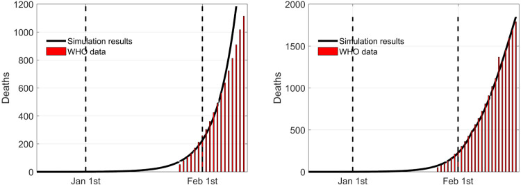
The values fixed for the parameters are in Table 1 having in mind the Hubei region case. Some of them have been defined on the basis of the information provided by the World Health Organization and from literature like [14], where numerical estimation were performed on the basis of the initial Chinese data. In addition, specific parameters identification has been performed to make the successive simulation results realistic and to put in evidence the advantages of the explicit and detailed introduction of the control actions. To this aim, a first estimation has been performed making use of data referred to the days before the first containment intervention, introduced on January 23, with invitation to limit the city circulation. The fitting of the numerical results for the uncontrolled dynamics is then expected to be acceptable until almost the end of January, being sure that after that date, a mismatch necessarily occurs due to the presence of the control action. In fact, a second time interval is considered, from the end of January on, assuming the action of the controls different from zero. In particular, a greater isolation of population and a more specific medication are considered, setting, from February 5, input $u_2$ equal to 0.8 (possibilities of contacts between individuals reduced to 20%), and $u_4$ equal to 0.4, (an improvement of 40% of the efficacy of the therapies for side effects). The effectiveness of the so obtained parameter values is evidenced by Fig. 2 where the number of death individuals are reported for the uncontrolled evolution of the disease (left) and the controlled one (right). Real data are represented by the vertical bars. The first figure show a good fitting for the first days until the control action is applied. The use of the modelled therapy control makes the correspondence between real and simulated data very good for the whole time interval considered. These considerations support the validation of the model to produce a very good fitting with the real case of the Hubei region in its first epidemic spread time.

Table 1.

Numerical values of the model parameters: comparative table for equivalent terms.

Parameter	B	$\beta$	k	$h_1$	$h_2$	$\gamma$
Value	1180	$2.5\cdot 10^{-8}$	1/7	$\varphi ∕3$	$(1-\varphi )∕15$	1/15
Parameter	$a$	$b$	$c$	$\eta$	n	$\varphi$
Value	$a$	$n∕15$	$1∕2$	$\eta$	0.95	0.9
Parameter	$d_S$	$d_E$	$d_{I_C}$	$d_{I_Q}$	$d_Q$	$d_R$
Value	$2\cdot 10^{-5}$	$2\cdot 10^{-5}$	$2\cdot 10^{-5}$	0.0057	$2\cdot 10^{-5}$	$2\cdot 10^{-5}$

Fig. 2.

Comparison between real data and model prevision without (left) and with (right) control actions for the number of deaths.

All the simulations have been performed starting from initial conditions $S\left(0\right)=59.17\cdot 10^6$, the population of the considered Wuhan region at the beginning of the epidemic, $E\left(0\right)=4$, $I_C\left(0\right)=2$, $I_Q\left(0\right)=1$, so that the results start with the discovery of the first positive patients, $Q\left(0\right)=0$ and $R\left(0\right)=0$.

3.2. Effects of preventive quarantine $u_1\left(t\right)$

The effects of the control action given by $u_1\left(t\right)$ is here presented and discussed.

This input corresponds to the choice of quarantining a fraction of the population because suspected to be infected or for a test campaign. Since the test campaign corresponds to the action modelled by the input $u_5\left(t\right)$, if only input $u_1\left(t\right)$ is active, only the isolation of suspected individuals is now considered. Such isolated individuals are kept in quarantine for a safe period (15 days), or until the symptoms appear.

In this short analysis, to better put in evidence if and when this action can be fruitful, two cases are considered: one in which the number of possible infected people among the quarantined is low, set equal to the 5% of them, and one on which the fraction of infected is higher, fixed to the 20%.

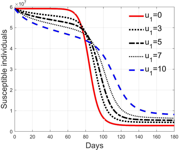
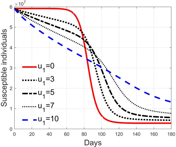
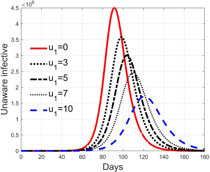
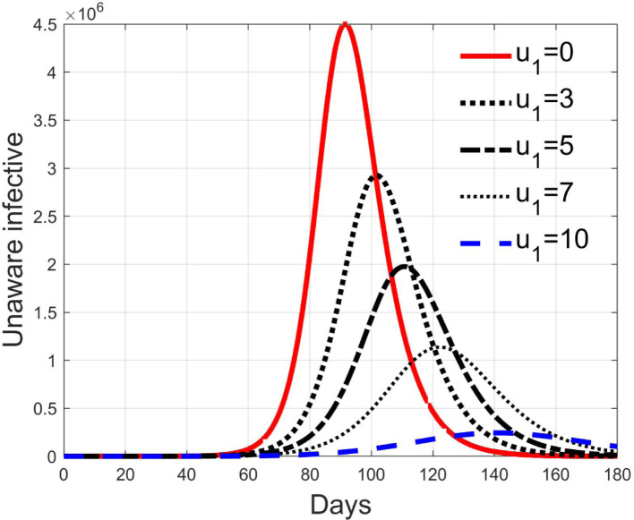
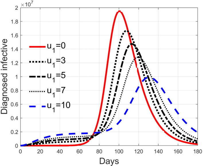
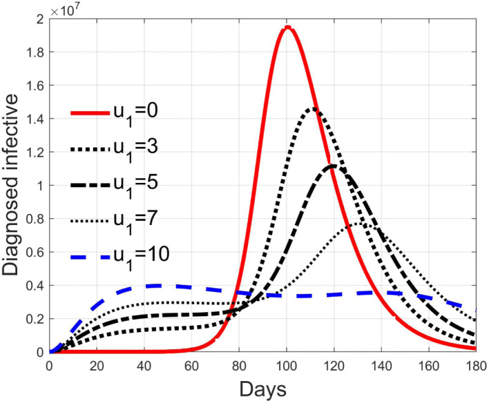
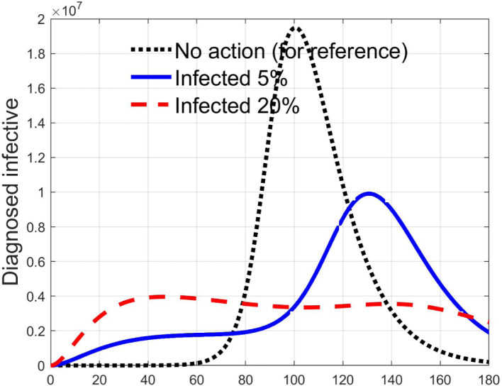
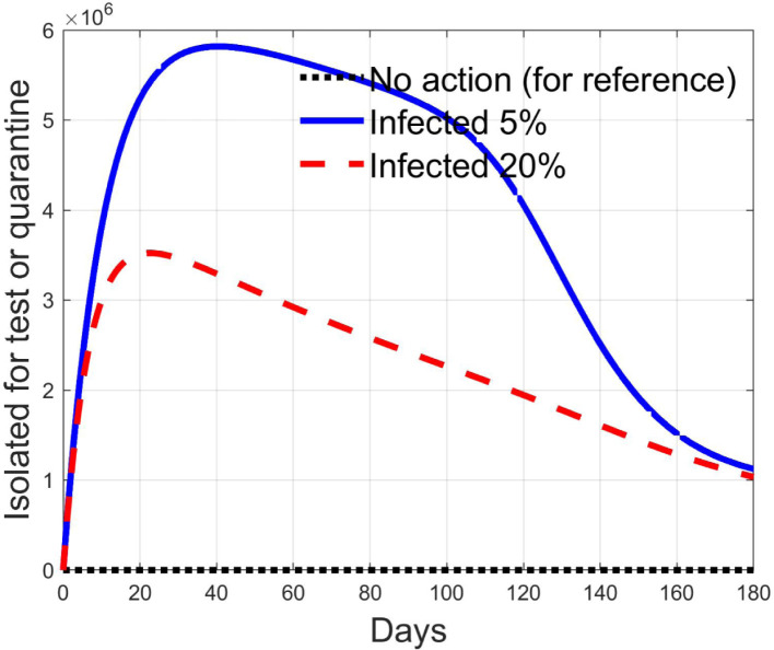
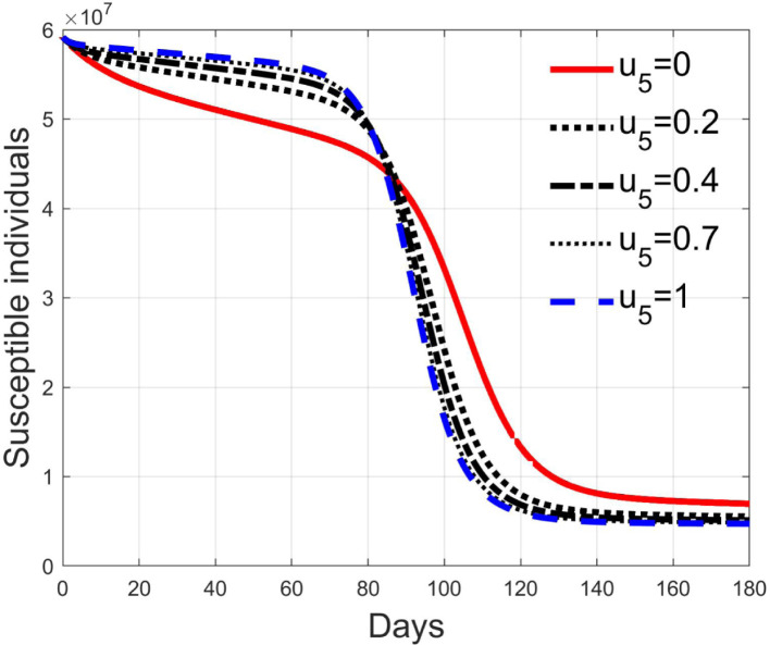
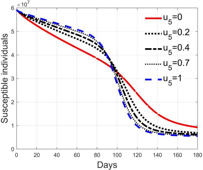
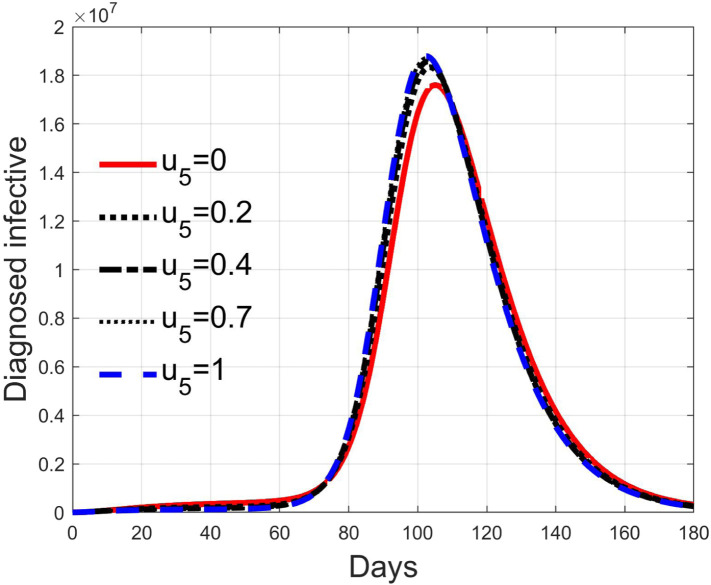
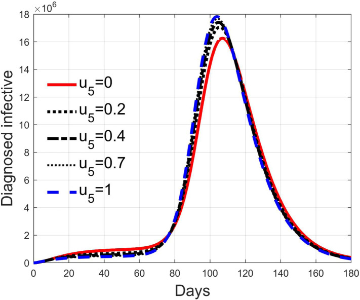
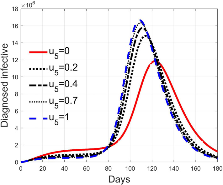
Simulations have been performed varying $u_1\left(t\right)$ between zero (no action) and 10; in Fig. 3, Fig. 4 the time history of the susceptible individuals is reported for the case of 5% and 20% of infected respectively. Clearly, the higher is the control amplitude, the higher is the initial decrement of the class due to the fact that a larger part is put in quarantine. However, this behaviour holds until the number of the infected individuals that can infect (i.e the ones before the symptoms or totally asymptomatic), increases, as can be observed from Fig. 5, Fig. 6. After the peak of infective persons, a higher control input produces a lower rate of decrement in the susceptible class. The important result arises from Fig. 7, Fig. 8 where the diagnosed infected individuals are reported for the two considered percentages. In fact, a delay of the peak as well as the reduction of its amplitude can be appreciated, more sensible for higher probability of infected individuals in the quarantined group, Fig. 8. This aspect is well evidenced in Fig. 9 where the case $u_1\left(t\right)=10$ is reported for the two cases of 5% and 20% of infected among the quarantined persons, along with the case of no action for reference purpose. It can be even observed a sort of flattening in the time evolution of the diagnosed infected patients exceptional for high rate of quarantine and high probability to have an infected individual in the quarantined group. With this action, the number of individuals put in quarantine, depicted in Fig. 10 for the same cases as in Fig. 9, presents a significant level, more acceptable when the infection probability is higher. In fact, for the two cases here addressed, when the percentage of infected patients is 5%, the value of more than the 8% of the initial population (about 5 millions) for more than 90 days is reached, while when 20% is considered, the maximum value assumed is 3.5 millions and decreases at a rate of more than 16600 a day.

Fig. 3.

Susceptible individuals for different amplitude of control $u_1\left(t\right)$ when 5% of quarantined is infected.

Fig. 4.

Susceptible individuals for different amplitude of control $u_1\left(t\right)$ when 20% of quarantined is infected.

Fig. 5.

Infected asymptomatic individuals for different amplitude of control $u_1\left(t\right)$ when 5% of quarantined is infected.

Fig. 6.

Infected asymptomatic individuals for different amplitude of control $u_1\left(t\right)$ when 20% of quarantined is infected.

Fig. 7.

Infected diagnosed individuals for different amplitude of control $u_1\left(t\right)$ when 5% of quarantined is infected.

Fig. 8.

Infected diagnosed individuals for different amplitude of control $u_1\left(t\right)$ when 20% of quarantined is infected.

Fig. 9.

Comparison between infected diagnosed individuals for the 5% and 20% cases of quarantined infected, when $u_1=10$.

Fig. 10.

Comparison between quarantined individuals for the 5% and 20% cases among them, when $u_1=10$.

3.3. Effects of isolation $u_2\left(t\right)$

Control $u_2\left(t\right)$ represents an action aiming at reducing the contact rate between susceptible and infected individuals. This can be obtained by means of a generalised quasi-isolation of the population, for example suggesting or imposing to people to stay at their own home as much time as possible, closing some activities like schools, offices, factories, shops and so on, so decreasing the possibilities of contacts.

Its effect reduces the nominal contact rate $\beta$. Thanks to the relationship between $\beta$ and $R_0$, it is possible to compute the minimum value for $u_2\left(t\right)$ to obtain a basic reproduction number smaller than 1 once the epidemic characteristic of the transmission, given by $\beta$, is fixed. In fact, it is possible to write

$${\tilde{R}}_0=\frac{\beta (1-u_2)kB}{d_S(k+d_E)(h_1+h_2+d_{I_C})}=R_0(1-u_2)$$ (40)

where $R_0$ is the initial reproduction number and ${\tilde{R}}_0<R_0$ is the one resulting under the action of the control. Then

$$u_2=1-\frac{{\tilde{R}}_0}{R_0}$$ (41)

and the lowest value $u_{2,min}$ to have ${\tilde{R}}_0\le 1$ is given by

$$u_{2,min}=1-\frac{1}{R_0}=0.6875$$ (42)

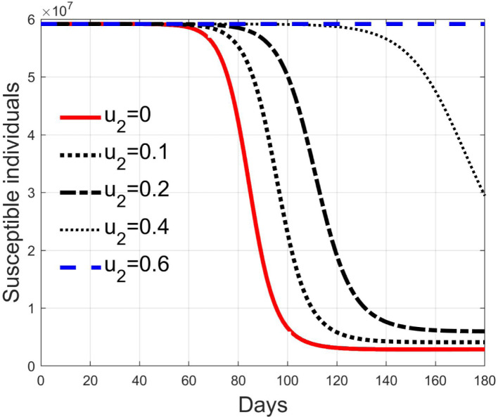
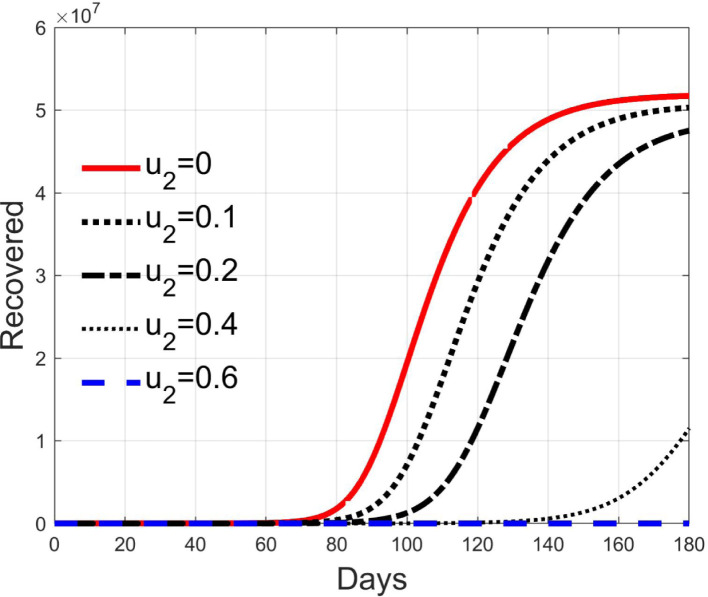
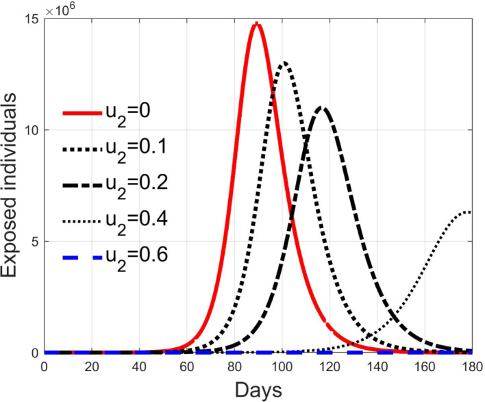
In Fig. 11, Fig. 12, Fig. 13, Fig. 14, Fig. 15 the results of simulation for different values of $u_2\left(t\right)\in [0,0.6]$ are reported. The five situations considered correspond to cases of epidemic with ${\tilde{R}}_0=R_0=3.2$ ($u_2=0$), ${\tilde{R}}_0=0.9R_0=2.88$ ($u_2=0.1$), ${\tilde{R}}_0=0.8R_0=2.56$ ($u_2=0.2$), ${\tilde{R}}_0=0.6R_0=1.92$ ($u_2=0.4$) and ${\tilde{R}}_0=0.4R_0=1.28$ ($u_2=0.6$). In fact, the curves in each figure have the same shape as epidemic spreads with different reproduction number. Then, it can be concluded that increasing $u_2\left(t\right)$, the spread is reduced and delayed in time, making the epidemic more controllable. For values sufficiently high, greater than $u_{2,min}$, the epidemic dynamics changes its characteristics and the disease free equilibrium becomes stable. It is interesting to note the correspondence of expression (42) with the condition for herd immunity.

Fig. 11.

Susceptible individuals for different values of $u_2\left(t\right)$.

Fig. 12.

Recovered individuals for different values of $u_2\left(t\right)$.

Fig. 13.

Exposed individuals for different values of $u_2\left(t\right)$.

Fig. 14.

Infected asymptomatic individuals for different values of $u_2\left(t\right)$.

Fig. 15.

Infected diagnosed individuals for different values of $u_2\left(t\right)$.

3.4. Effects of antiviral therapy $u_3\left(t\right)$

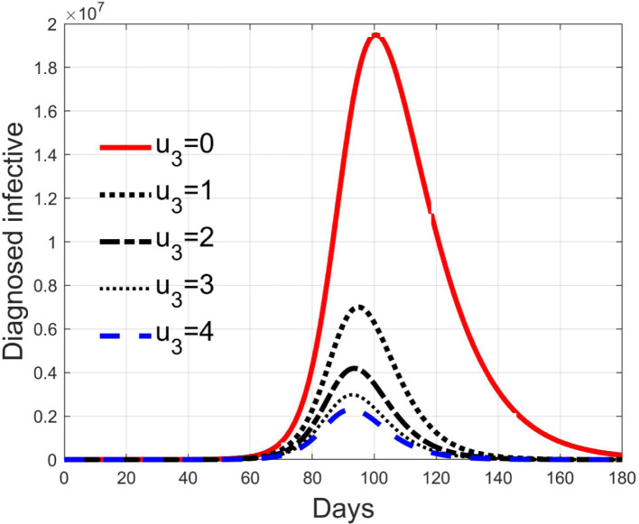
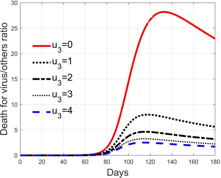
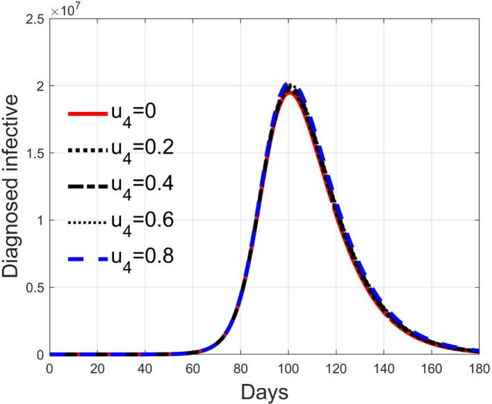
The control $u_3\left(t\right)$ acts on the diagnosed infected patients to reduce and contrast the virus effects so facilitating and reducing the time for healing. Fig. 16 depicts the time history of the number of such patients for the cases of $u_3\left(t\right)=0,1,2,3,4$. Thanks to the direct effect of such a control, the peak values are strongly reduced with consequences on the number of deaths, as can be noted in Fig. 17, where the ratio between the deaths of infected patients and the standard deaths is plotted. This result shows that, if available, an antiviral therapy produces highly positive effects for the infection contrast.

Fig. 16.

Infected diagnosed individuals for different values of control $u_3\left(t\right)$.

Fig. 17.

Ratio between deaths by virus and other deaths, for different values of control $u_3\left(t\right)$.

3.5. Effects of therapy against complications $u_4\left(t\right)$

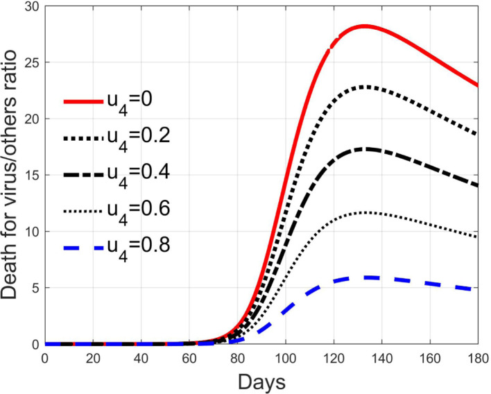
Like the previous one, the control $u_4\left(t\right)$ acts on the diagnosed infected patients but, differently from $u_3\left(t\right)$, it represents the efficacy of the therapy against the effects induced by the virus and for the possible complications. Its goal is to keep alive the patient during the natural development and evolutions of the individual anti-viruses, for example with intensive care and respiratory supports. The consequence is that it reduces the death rate, as depicted in Fig. 18, but it does not affect sensibly the number of isolated and treated individuals, as seen in Fig. 19 since, differently from the case of input $u_3\left(t\right)$, this action does not remove more quickly patients from the class but keeps them there for all the illness period. In Fig. 18 it is clear the reduction of the deaths, 28 times the normal quantities at the peak with $u_4\left(t\right)=0$, which becomes 6 times with $u_4\left(t\right)=0.8$, decreasing almost linearly.

Fig. 18.

Ratio between deaths by virus and other deaths, for different values of control $u_4\left(t\right)$.

Fig. 19.

Infected diagnosed individuals for different values of control $u_4\left(t\right)$.

3.6. Effects of amount of tests $u_5\left(t\right)$

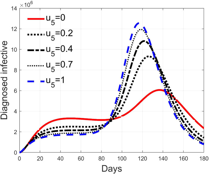
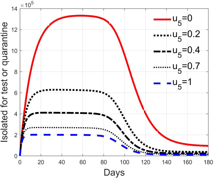
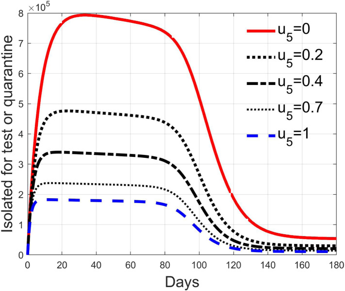
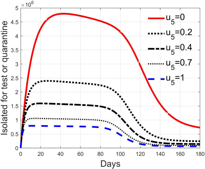
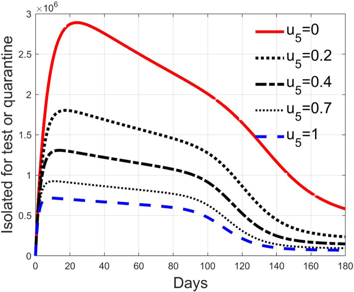
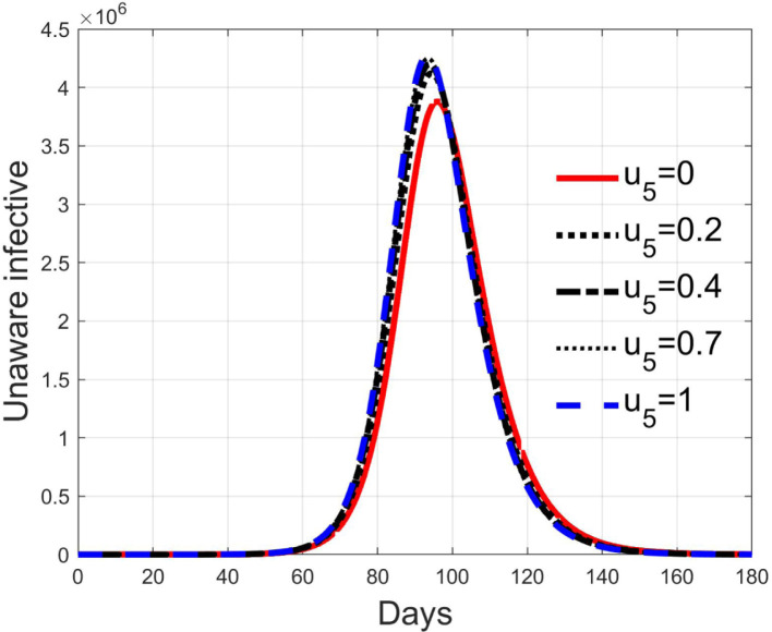
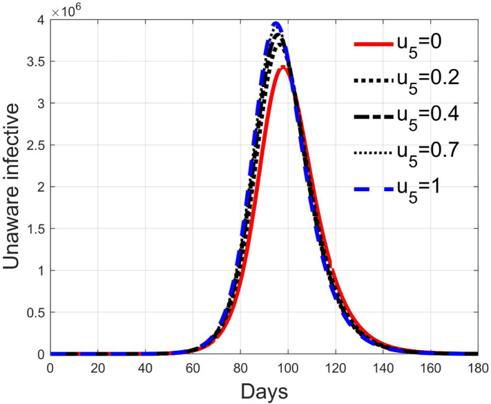
The control input $u_5\left(t\right)$ represents the amount of test performed on the population. In this model, the people to be tested are temporarily considered as quarantined. Moving people to quarantine status can be done by means of input $u_1$ only. Then, in order to analyse the effect of different levels of test rate, the input $u_1\left(t\right)$ must be set to a value different to zero. Moreover, as remarked in Section 3.2, the effect of putting persons in quarantine is dependent on the hypothesised number of positive results.

These considerations motivate the choice of four cases, obtained combining the cases of high and low value for $u_1\left(t\right)$, chosen equal to 2 and 8 respectively, with the cases of high and low percentage of expected positive tests, the two already considered values of 20% and 5%. For each of these four cases, the input $u_5\left(t\right)$ is varied in the interval $[0,1]$.

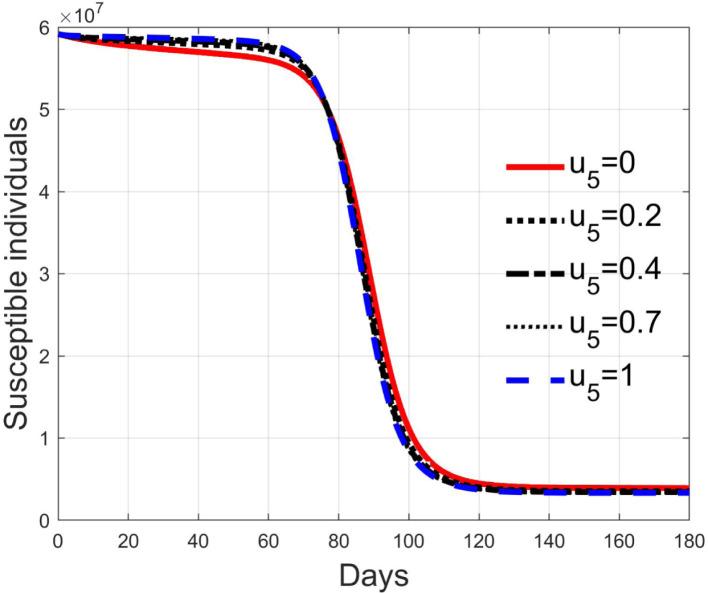
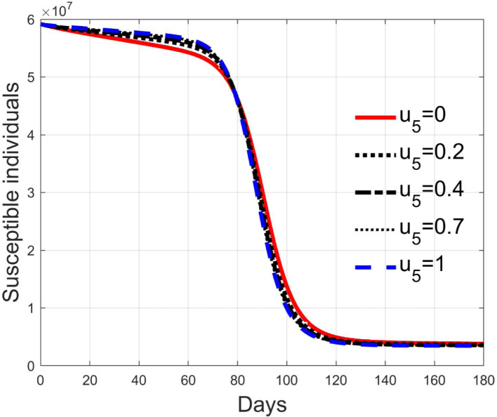
In Fig. 20, Fig. 21, Fig. 22, Fig. 23 the effects on the susceptible class are presented. Fig. 20, Fig. 21 both refer to the case of low rate of motion to the quarantine status ($u_1\left(t\right)=2$, 0.2% of susceptible people a day), the first one for a low fraction of infected (5%, $n=0.95$) and the second one for a high number (20%, $n=0.8$). Fig. 22, Fig. 23 have the same meaning but with a higher rate of transfer to quarantine for test ($u_1\left(t\right)=8$).

Fig. 20.

Susceptible individuals $S$ for low rate of quarantine transfer ($u_1\left(t\right)=2$) and low percentage of infected among them (5%).

Fig. 21.

Susceptible individuals $S$ for low rate of quarantine transfer ($u_1\left(t\right)=2$) and high percentage of infected among them (20%).

Fig. 22.

Susceptible individuals $S$ for high rate of quarantine transfer ($u_1\left(t\right)=8$) and low percentage of infected among them (5%).

Fig. 23.

Susceptible individuals $S$ for high rate of quarantine transfer ($u_1\left(t\right)=8$) and high percentage of infected among them (20%).

Fig. 28, Fig. 29, Fig. 30, Fig. 31 depict the diagnosed infected patients, while Fig. 32, Fig. 33, Fig. 34, Fig. 35 refer to the quarantined individuals, always with the same order for $u_1\left(t\right)$ and $n$ as for the susceptible individuals.

Fig. 28.

Infected diagnosed individuals $I_Q$ for low rate of quarantine transfer ($u_1\left(t\right)=2$) and low percentage of infected among them (5%).

Fig. 29.

Infected diagnosed individuals $I_Q$ for low rate of quarantine transfer ($u_1\left(t\right)=2$) and high percentage of infected among them (20%).

Fig. 30.

Infected diagnosed individuals $I_Q$ for high rate of quarantine transfer ($u_1\left(t\right)=8$) and low percentage of infected among them (5%).

Fig. 31.

Infected diagnosed individuals $I_Q$ for high rate of quarantine transfer ($u_1\left(t\right)=8$) and high percentage of infected among them (20%).

Fig. 32.

Quarantined individuals $Q$ for low rate of quarantine transfer ($u_1\left(t\right)=2$) and low percentage of infected among them (5%).

Fig. 33.

Quarantined individuals $Q$ for low rate of quarantine transfer ($u_1\left(t\right)=2$) and high percentage of infected among them (20%).

Fig. 34.

Quarantined individuals $Q$ for high rate of quarantine transfer ($u_1\left(t\right)=8$) and low percentage of infected among them (5%).

Fig. 35.

Quarantined individuals $Q$ for high rate of quarantine transfer ($u_1\left(t\right)=8$) and high percentage of infected among them (20%).

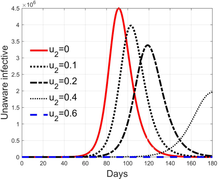
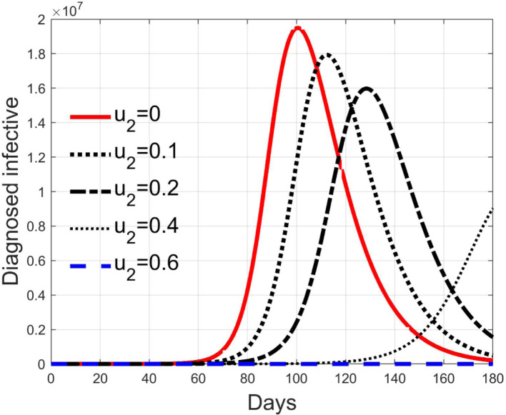
Recalling that the case of $u_5\left(t\right)=0$ refers to a pure quarantine policy, analysed in Section 3.2, the most evident result is that, testing the quarantined persons and letting the negative ones return to the susceptible class has the consequence to increase the epidemic spread from the outbreak of the virus until the peak of the infection, anticipated in time and increased in amplitude. In fact, in this time interval, the number of susceptible persons decreases slower as $u_5\left(t\right)$ increases, as observable in Fig. 20, Fig. 21, Fig. 22, Fig. 23, since a high number of tests let many negative individuals return in such a class instead of remaining in the quarantine one longer. Even if some exposed and asymptomatic subjects are found and isolated, the decrement of the infective individuals is compensated by the increment of the susceptible persons, in Fig. 24, Fig. 25, Fig. 26, Fig. 27, with the consequence of having more infected patients. During this time, the number of diagnosed individuals is lower, Fig. 28, Fig. 29, Fig. 30, Fig. 31, probably because the total time of transition from the susceptible to the diagnosed class for all the not tested individuals is longer than from quarantine to diagnosis class.

Fig. 24.

Infective individuals $I_C$ for low rate of quarantine transfer ($u_1\left(t\right)=2$) and low percentage of infected among them (5%).

Fig. 25.

Infective individuals $I_C$ for low rate of quarantine transfer ($u_1\left(t\right)=2$) and high percentage of infected among them (20%).

Fig. 26.

Infective individuals $I_C$ for high rate of quarantine transfer ($u_1\left(t\right)=8$) and low percentage of infected among them (5%).

Fig. 27.

Infective individuals $I_C$ for high rate of quarantine transfer ($u_1\left(t\right)=8$) and high percentage of infected among them (20%).

In correspondence of the peak of infected, the number of susceptible persons presents a fast decrement, as usual in epidemics spread, but in this case the velocity of the decrement is directly related to the number of tests. From the point of view of the diagnosed infective patients, after the initial period with a slow increment, the evolution follows the same behaviour as all the infected classes, with its peak and the subsequent decrement.

The quarantined class is highly affected by the different choices, as Fig. 32, Fig. 33, Fig. 34, Fig. 35 show. In fact, it can be appreciated how much the number of tests contributes to the class emptying.

This phenomenon is related to the initial behaviour of the diagnosed individuals discussed above: emptying the quarantine class corresponds to reduce the isolation and to have, along the illness course, the asymptomatic infective class more filled, with consequences on the velocity of the spread.

4. Two real cases

After having described the general behaviour of the system under possible values of the controls, the real cases of two European Countries is here faced. One is Italy, characterised by more than two months of hard lockdown, and the other is United Kingdom, with milder restrictions.

The aim of this analysis is twofold. The first goal is to further validate the model proposed over a long time evolution and under changes of the control over time. The second one is to show the capabilities of the mathematical model to capture and describe the actual effects of the policies adopted by each Country, performing such a validation for two dimensionally equivalent Countries with different epidemic containment choices of the Governments. This, conversely, corresponds to the ability of the model to describe in a very accurate and reliable way the effects of the control actions.

For both the studies, data have been collected from nationalorganisations (http://www.protezionecivile.gov.it/ for Italy, https://coronavirus.data.gov.uk/ for United Kingdom) and verified on the basis of the COVID-19 bulletins of the World Health Organization (https://www.who.int/).

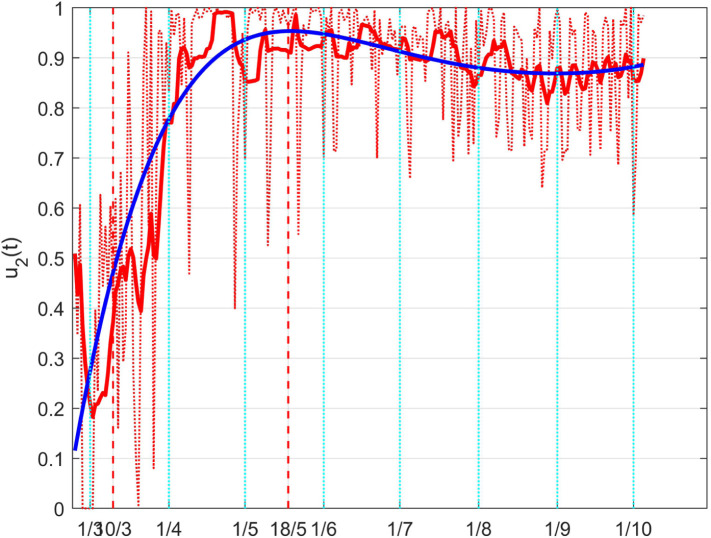
The identification process has been performed with a least square error approach on the number of infected and dead individuals, the most commonly available data. Consequently, the analysis has been focused on the control $u_2\left(t\right)$, the most directly involved with the virus spread and then the number of infected, and the control $u_4\left(t\right)$, related with the medical assistance of the symptomatic hospitalised people at risk of death.

4.1. The Italian case

Data available for Italy starts from February 24, so all the graphs start from that date.

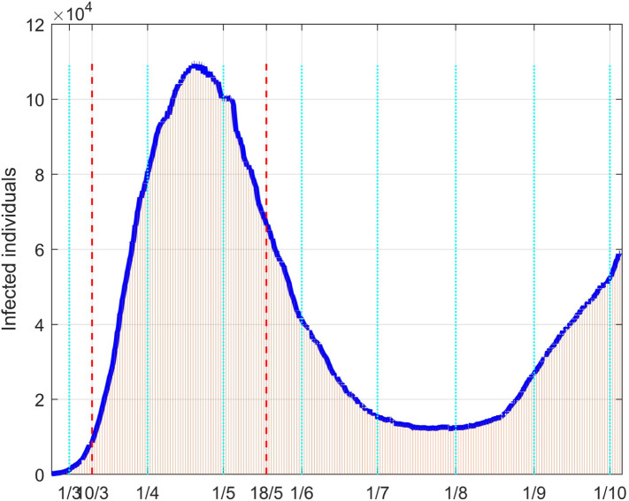
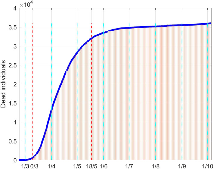
Fig. 36, Fig. 37 depict the results of the model fitting procedure. The correspondence of the simulated data with the real ones shows that the mathematical model is capable to describe the actual behaviour of the epidemic evolution once a time varying control action is properly considered in the model.

Fig. 36.

Infected people in Italy: real data (daily vertical red bars) and model fitting (solid blue line).

Fig. 37.

Dead people in Italy: real data (daily vertical red bars) and model fitting (solid blue line).

In fact, in Fig. 38 the time evolution of the control $u_2\left(t\right)$ is plotted. The initially estimated values are reported with the dotted red line. It is characterised by an expected flickering evolution; this is mainly due to the presence on the data of a large noise caused by how they are collected, for example on the basis of a daily variable number of tests, and for the presence of non smooth effects produced by the clusters-based diffusion of the virus. In fact, it is sufficient to consider average values, for example over ten days, to obtain a clearer evolution, as depicted with the red solid line.

Fig. 38.

The Italian case: time history of the control $u_2\left(t\right)$. Dotted red graph: noise affected estimation of the control; red solid line: ten days average filtering for noise reduction; blue solid line: interpolation with a polynomial of degree five.

A polynomial interpolation of the estimated samples for the daily values of the control $u_2\left(t\right)$ show a clear evolution of the actual control applied.

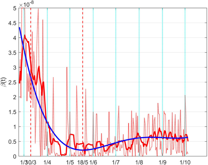
To confirm the correctness of the results, it can be noted that during the lockdown period, evidenced in all the Figures between the vertical dashed lines, the control quickly increases reaching its maximum, and then, after the relaxation of the constraints, it reduces.

A more immediate idea of such a result can be given depicting the so obtained full coefficient $\beta (1-u_2\left(t\right))$, which can be interpreted as a time varying coefficient $\beta \left(t\right)$. This is done in Fig. 39, where the meaning of the different lines is the same as in the previous Figure; its interpretation is more intuitive: the decrement, with the achievement of its minimum during the lockdown, and the subsequent rise.

Fig. 39.

The Italian case: time history of the controlled coefficient $\beta \left(t\right)$. Dotted red graph: noise affected estimation of the value; red solid line: ten days average filtering for noise reduction; blue solid line: interpolation with a polynomial of degree five.

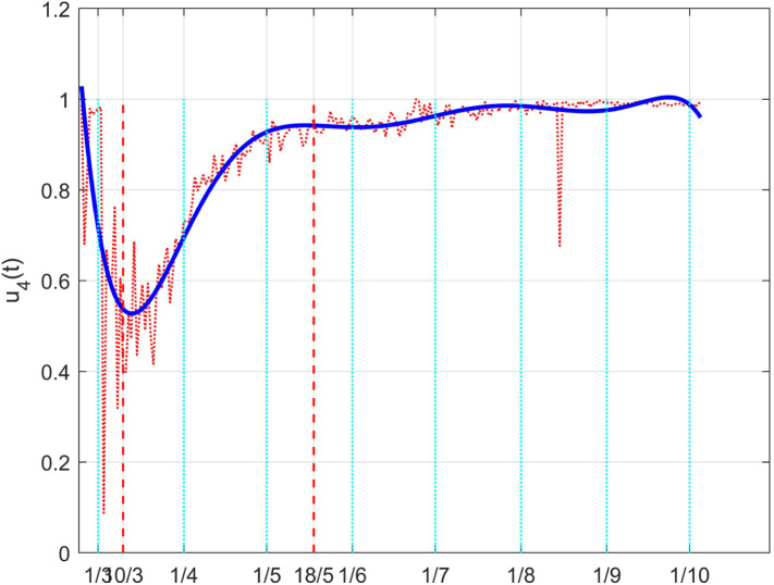
A similar approach can be adopted for the control $u_4\left(t\right)$. Fig. 40 depicts the raw estimated values for the therapy action and its approximation with a polynomial of degree five. Its physical correspondence with the actual behaviour is evidenced by the fact that it is characterised by a high value, which means a full effectiveness of the therapies, except in the initial period of the lockdown, where the high number and rate of hospitalisations reduced the capabilities of a fully effective action. The introduction of the lockdown had also the positive effect to increase the medical action, making it return to the normal high effect.

Fig. 40.

The Italian case: time history of the control $u_4\left(t\right)$. Dotted red graph: noise affected estimation of the control; blue solid line: interpolation with a polynomial of degree five.

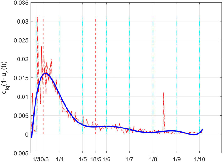
As for $u_2\left(t\right)$, the effect of the changes in $u_4\left(t\right)$ can be better evidenced from the time history of the full death coefficient $d_{Iq}(1-u_4\left(t\right))$ depicted in Fig. 41. The higher rate of death before the lockdown and the decrement during that containment period are well evident.

Fig. 41.

The Italian case: time history of the controlled coefficient $d_{Iq}\left(t\right)$. Dotted red graph: noise affected estimation of the value; blue solid line: interpolation with a polynomial of degree five.

4.2. The United Kingdom case

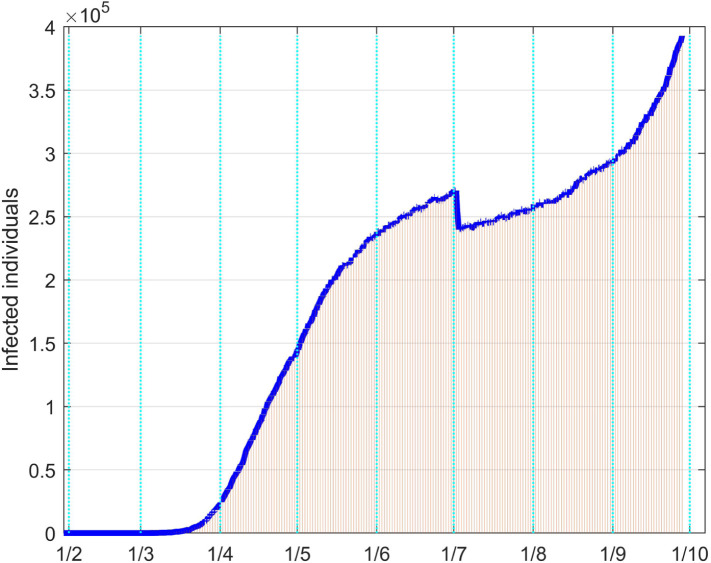
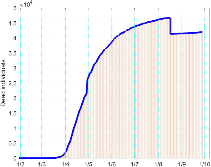
For the United Kingdom analysis, available data have been collected since February 1. The same identification approach as for the Italian case has been performed. The fitting results for the infective and the dead individuals are reported in Fig. 42, Fig. 43 respectively.

Fig. 42.

Infected people in UK: real data (daily vertical red bars) and model fitting (solid blue line).

Fig. 43.

Dead people in UK: real data (daily vertical red bars) and model fitting (solid blue line).

Since no strong limitations have been adopted by the Government, the number of infected people is monotonically increased, with different rates, as well as the one of the dead patients. The two discontinuities on the data sequences are motivated by changes in the data acquisition or evaluation. For example, the decrement of about five thousand units for the dead evaluations comes from the fact that from August 15 only the persons for which COVID-19 is the main death cause are counted, while before that day all the dead people positive to the virus were included.

As for the Italian case, the fitting is very satisfactory, since time varying controls are assumed.

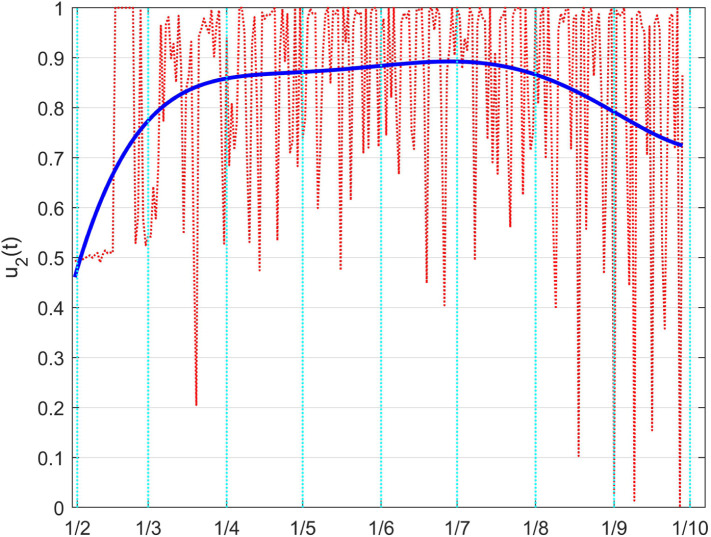
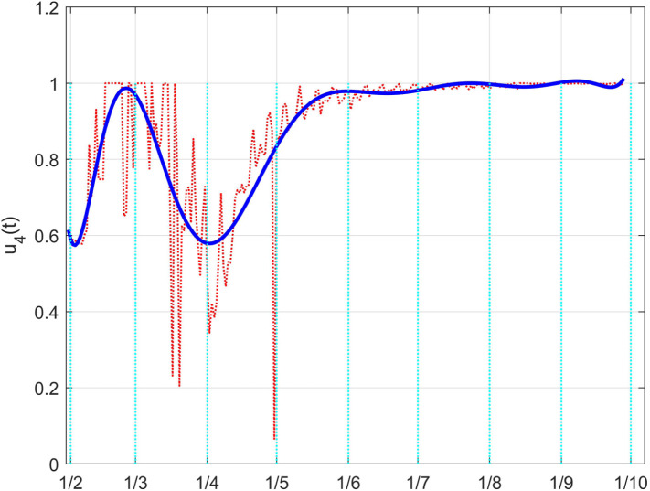
Time histories of such controls are reported in Fig. 44 for $u_2\left(t\right)$ and in Fig. 45 for $u_4\left(t\right)$.

Fig. 44.

The UK case: time history of the control $u_2\left(t\right)$. Dotted red graph: noise affected estimation of the control; blue solid line: interpolation with a polynomial of degree five.

Fig. 45.

The UK case: time history of the control $u_4\left(t\right)$. Dotted red graph: noise affected estimation of the control; blue solid line: interpolation with a polynomial of degree five.

From Fig. 44 it is evident a decrement of the contact reduction starting from last Summer (August 2020), which finds the physical confirmation in the strong increment of positive cases (Fig. 42); a second observation arises comparing Fig. 44 with the corresponding one, Fig. 38, in the Italian case; there is a generalised lower effort of this control action, almost constant over a long period, without peaks from high social restrictions, and a sensible constant reduction of amplitude in the last two months: this motivates the slope of the infected individuals count in Fig. 42 in the corresponding time interval.

Fig. 45 shows a situation for the control $u_4\left(t\right)$ very similar to the Italian case. A general high effectiveness of the therapies on hospitalised individuals with severe effects of the infections is evidenced, except for the interval March–April, during the initial fast spread of the virus and the pandemic declaration. According to the general illustrations in Sections 3.3, 3.5, the indirect effect of the Italian lockdown in the therapies effectiveness produced a shorter time interval of the lower effort (the pits in the graphs) than in UK: they both started in March but fully ended at the beginning of May for Italy, while it lasted until the second half of May for UK.

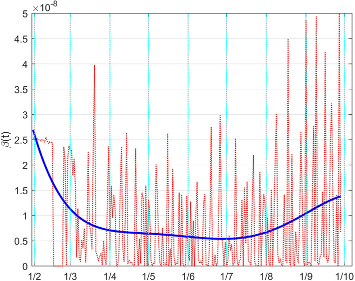
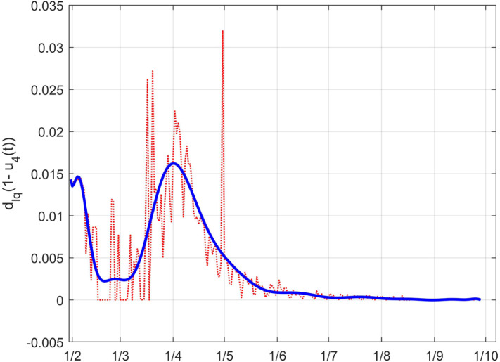
Reporting these results on the model coefficients, the time variation of the effective transmission rate, $\beta \left(t\right)=\beta (1-u_2\left(t\right))$ in Fig. 46, and the dead coefficient, $d_{Iq}(1-u_4\left(t\right))$ in Fig. 47, can give a more direct evaluation of the effects of the two controls. A reduction of the transmission rate characterises the time from March to July, while a continuous dangerous increment is evident from middle July on.

Fig. 46.

The UK case: time history of the controlled coefficient $\beta \left(t\right)$. Dotted red graph: noise affected estimation of the value; blue solid line: interpolation with a polynomial of degree five.

Fig. 47.

The UK case: time history of the controlled coefficient $d_{Iq}\left(t\right)$. Dotted red graph: noise affected estimation of the value; blue solid line: interpolation with a polynomial of degree five.

Luckily, this recent increment is not impacting, till now, on the medical capability of diseased individuals, as evidenced by the flatness in Fig. 47 from June on, with a very low dead coefficient.

5. Conclusions

In this paper, a new mathematical model for describing the spread of a virus, in absence of vaccination and a with significant presence of hidden infective individuals, is introduced for the analysis of the effects of possible control strategies.

The model is designed to include all the suitable active actions, both from the political point of view and the medical one, whose implementation can involve complex aspects of social behaviour and individual response.

The model proposed wants to be a reference for political and administrative heads to define control strategies, once the economical and social costs, associated to the inputs and their consequences, are chosen. Due to this high level decision dependence, a general analysis for the characterisation of the effects is here performed, showing their consequences on the different modelled classes of population.

In order to validate the model here presented, its adaptation to the behaviour of the COVID-19 in the Wuhan region at the beginning of the infection spread is presented. This procedure is applied for tuning the model parameters in the almost unique case of absence of control, and for showing the role of the inputs to describe the effects of the initial decisions of the Chinese Government.

The approach followed is based on the graphical comparison of numerical simulations obtained under different values of control efforts, in order to produce intuitive and easy to see results that could better take into account not modelled human behaviours.

This analysis can be a supporting tool to adopt possible choices having a clearer vision of the effects not only for the intuitive cases, as in Section 3.3, but, more important, for the not obvious behaviours, described in Section 3.6, coherent with the opinion of many experts which propose a massive test campaign for virus spread containment.

For example, it can be useful to state the maximum levels of available medical cares to define the isolation and the quarantine actions; moreover, it can support the evaluation of the economic effects produced by lockdown policies.

For the COVID-19, the validity of the model as well as its capability of describing the effects of the controls in real situations are supported by analysing the cases of two different Countries, Italy and United Kingdom, showing the correspondences between the model evolutions and the real epidemic behaviours. These two Countries, comparable for geographical, cultural and demographical aspects, are characterised by strongly different initial approaches for facing the pandemic: a national hard lockdown for Italy, with respect to an initial choice, for UK, to avoid restrictive containment measures, aiming at a heard immunity condition.

The interesting aspects of the results here presented, supported by the satisfactory fitting of the epidemic evolution in different environments, are twofold: starting from the actual situation, it is possible to establish a correspondence between changes in the containment measures and expected epidemic evolution; this allows to predict the consequences of different choices of action strategies (level of restrictions on people interaction, lockdown, tests, hospital facilities, …) and, conversely, to suggest and support the most suitable lines of intervention, once target conditions are provided.

Note that this model, designed and tuned for the ongoing COVID-19 emergency, for its structure can be adopted also for other epidemic diseases in which there is a significant presence of unaware infected individuals which increase the virus spread.

Declaration of Competing Interest

The authors declare that they have no known competing financial interests or personal relationships that could have appeared to influence the work reported in this paper.

References

- 1.Kermack W.O., McKendrick A.G. A contribution to the mathematical theory of epidemics. Proc. R. Soc. Lond. A. 1927;115(772):700–721. [Google Scholar]
- 2.Naresh R., Tripathi A., Sharma D. Modeling and analysis of the spread of AIDS epidemic with immigration of HIV infectives. Math. Comput. Modelling. 2009;49:880–892. [Google Scholar]
- 3.T. Vasanthi, V. Vijayalakshmi, Mathematical models for the study of HIV/AIDS epidemics, in: Proc. IEEE International Conference on advances in Engineering, Science and Management, 2012, pp. 108–112.
- 4.Basak U.S., Datta B.K., Ghose P.K. Mathematical analysis of an HIV/AIDS epidemic model. Amer. J. Math. Stat. 2015;5(5):253–258. [Google Scholar]
- 5.Di Giamberardino P., Iacoviello D. 22nd International Conference on System Theory, Control and Computing. 2018. Optimal control to reduce the HIV/AIDS spread; pp. 87–92. [Google Scholar]
- 6.Di Giamberardino P., Compagnucci L., De Giorgi C., Iacoviello D. Modeling the effects of prevention and early diagnosis on HIV/AIDS infection diffusion. IEEE Trans. Syst. Man Cybern.: Syst. 2019:2119–2130. [Google Scholar]
- 7.Di Giamberardino P., Iacoviello D. Epidemic modeling and control of HIV/AIDS dynamics in populations under external interactions: a worldwide challenge. Control Appl. Biomed. Eng. Syst. Elsevier. 2020 [Google Scholar]
- 8.Perry R.T., Halset N.A. The clinical significance of measles: a review. J. Infec. Dis. 2004;189(1):4–16. doi: 10.1086/377712. [DOI] [PubMed] [Google Scholar]
- 9.Onyejekwe O.O., Kebede E.Z. Epidemiological modeling of measles infection with optimal control of vaccination and supportive treatment. Appl. Comput. Math. 2015;4(4):264–274. [Google Scholar]
- 10.Adewale S.O., Olopade I.A., Ajao S.O., Adeniran G.A. Optimal control analysis of the dynamical spread of measles. Int. J. Res. 2016;4(5):169–188. [Google Scholar]
- 11.Di Giamberardino P., Iacoviello D. ICINCO 2019 - Proceedings of the 16th International Conference on Informatics in Control, Automation and Robotics, Vol. 1. 2019. Analysis, simulation and control of a new measles epidemic model; pp. 550–559. [Google Scholar]
- 12.P. Di Giamberardino, D. Iacoviello, Modeling and control of an epidemic disease under possible complication, in: Proceedings of the 22nd International Conference on System Theory, Control and Computing, 2018, pp. 67–72.
- 13.Lai C.-C., Shih T.-P., Ko W.-C., Tang H.-J., Hsueh P.-R. Severe acute respiratory syndrome coronavirus 2 (SARS-CoV-2) and coronavirus disease-2019 (COVID-19): The epidemic and the challenges. Int. J. Antimicrob. Ag. 2020;55(3):1–9. doi: 10.1016/j.ijantimicag.2020.105924. [DOI] [PMC free article] [PubMed] [Google Scholar]
- 14.Tang B., Wang X., Li Q., Bragazzi N.L., Tang S., Xiao Y., Wu J. Estimation of the transmission risk of the 2019-nCoV and its implication for public health interventions. J. Clin. Med. 2020;9(2) doi: 10.3390/jcm9020462. [DOI] [PMC free article] [PubMed] [Google Scholar]
- 15.Tang B., Bragazzi N.L., Li Q., Tang S., Xiao Y., Wu J. An updated estimation of the risk of transmission of the novel coronavirus (2019-ncov) Infec. Dis. Model. 2020;5:248–255. doi: 10.1016/j.idm.2020.02.001. [DOI] [PMC free article] [PubMed] [Google Scholar]
- 16.Wu J.T., Leung K., Leung G.M. Nowcasting and forecasting the potential domestic and international spread of the 2019-nCoV outbreak originating in Wuhan, China: a modelling study. Lancet. 2020 doi: 10.1016/S0140-6736(20)30260-9. [DOI] [PMC free article] [PubMed] [Google Scholar]
- 17.Zhao S., Lin Q., Musa J.R.S.S., Yang G., Wang W., Lou Y., Gao D., Yang L., He D., Wang M.H. Preliminary estimation of the basic reproduction number of novel coronavirus (2019-nCoV) in China, from 2019 to 2020: A data-driven analysis in the early phase of the outbreak. Int. J. Infec. Dis. 2020;92:214–217. doi: 10.1016/j.ijid.2020.01.050. [DOI] [PMC free article] [PubMed] [Google Scholar]
- 18.Zhanga S., Diaob M., Yuc W., Peic L., Lind Z., Chena D. Estimation of the reproductive number of Novel Coronavirus (COVID-19) and the probable outbreak size on the Diamond Princess cruise ship: A data-driven analysis. Int. J. Infec. Dis. 2020 doi: 10.1016/j.ijid.2020.02.033. [DOI] [PMC free article] [PubMed] [Google Scholar]
- 19.Roosa K., Lee Y., Luo R., Kirpich A., Rothenberg R., Hyman J., Yan P., Chowell G. Real-time forecasts of the COVID-19 epidemic in China from February 5th to February 24th, 2020. Infec. Dis. Model. 2020;5:256–263. doi: 10.1016/j.idm.2020.02.002. [DOI] [PMC free article] [PubMed] [Google Scholar]
- 20.Arino J., Portet S. A simple model for COVID-19. Infec. Dis. Model. 2020;5:309–315. doi: 10.1016/j.idm.2020.04.002. [DOI] [PMC free article] [PubMed] [Google Scholar]
- 21.Liu Z., Magal P., Seydi O., Webb G. A COVID-19 epidemic model with latency period. Infec. Dis. Model. 2020;5:323–337. doi: 10.1016/j.idm.2020.03.003. [DOI] [PMC free article] [PubMed] [Google Scholar]
- 22.Chowell G., Hincapie-Palacio D., Ospina J., Pell B., Tariq A., Dahal S., Moghadas S., Smirnova A., Simonsen L., Viboud C. Using Phenomenological Models to characterize Transmissibility and forecast Patterns and Final Burden of Zika Epidemics. PLoS Curr. 2016;8 doi: 10.1371/currents.outbreaks.f14b2217c902f453d9320a43a35b9583. [DOI] [PMC free article] [PubMed] [Google Scholar]
- 23.Pell B., Kuang Y., Viboud C., Chowell G. Using phenomenological models for forecasting the 2015 Ebola challenge. Epidemics. 2018;22:62–70. doi: 10.1016/j.epidem.2016.11.002. [DOI] [PubMed] [Google Scholar]
- 24.Bürger R., Chowell G., Lara-Díıaz L.Y. Comparative analysis of phenomenological growth models applied to epidemic outbreaks. Math. Biosci. Eng. 2019;16(mbe-16-05-212):4250–4273. doi: 10.3934/mbe.2019212. [DOI] [PubMed] [Google Scholar]
- 25.Chowell G., Tariq A., Hyman J. A novel sub-epidemic modeling framework for short-term forecasting epidemic waves. BMC Med. 2019;17 doi: 10.1186/s12916-019-1406-6. [DOI] [PMC free article] [PubMed] [Google Scholar]
- 26.Cowling B.J., Ho L.M., Leung G.M. Effectiveness of control measures during the SARS epidemic in Beijing: a comparison of the curve and the epidemic curve. Epidemiol. Infect. 2008;136:562–566. doi: 10.1017/S0950268807008722. [DOI] [PMC free article] [PubMed] [Google Scholar]
- 27.Bakare E., Nwagwo A., Danso-Addo E. Optimal control analyis of an SIR epidemic model with constant recruitment. Int. J. Appl. Math. Res. 2014;3:275–285. [Google Scholar]
- 28.Di Giamberardino P., Iacoviello D. Optimal control of SIR epidemic model with state dependent switching cost index. Biomed. Signal Process. Control. 2017;31:377–380. [Google Scholar]
- 29.Di Giamberardino P., Iacoviello D., Papa F., Sinisgalli C. Dynamical evolution of COVID-19 in Italy with an evaluation of the size of the asymptomatic infective population. IEEE J. Biomed. Health Inform. (Early Access) 2020 doi: 10.1109/JBHI.2020.3009038. [DOI] [PMC free article] [PubMed] [Google Scholar]
- 30.Di Giamberardino P., Iacoviello D. 26th Mediterranean Conference on Control and Automation, MED 2018. 2018. An output feedback control with state estimation for the containment of the HIV/AIDS diffusion; pp. 192–197. [Google Scholar]
- 31.Di Giamberardino P., Iacoviello D. 22nd International Conference on System Theory, Control and Computing (ICSTCC) 2018. Optimal control to reduce the HIV/AIDS spread; pp. 87–92. [Google Scholar]
- 32.Mandal M., Jana S., Nandi S.K., Khatua A., Adak S., Kar T. A model based study on the dynamics of COVID-19: Prediction and control. Chaos Solitons Fractals. 2020;136 doi: 10.1016/j.chaos.2020.109889. [DOI] [PMC free article] [PubMed] [Google Scholar]
- 33.Daley D.J., Gani J. Epidemic Modelling: An Introduction. Cambridge University Press; 1999. (Cambridge Studies in Mathematical Biology). [Google Scholar]
- 34.Martcheva M. vol. 61. Springer; 2015. An introduction to mathematical epidemiology. (Text in Applied Mathematics). [Google Scholar]