Semantic Segmentation of Smartphone Wound Images: Comparative Analysis of AHRF and CNN-Based Approaches

Abstract

Smartphone wound image analysis has recently emerged as a viable way to assess healing progress and provide actionable feedback to patients and caregivers between hospital appointments. Segmentation is a key image analysis step, after which attributes of the wound segment (e.g. wound area and tissue composition) can be analyzed. The Associated Hierarchical Random Field (AHRF) formulates the image segmentation problem as a graph optimization problem. Handcrafted features are extracted, which are then classified using machine learning classifiers. More recently deep learning approaches have emerged and demonstrated superior performance for a wide range of image analysis tasks. FCN, U-Net and DeepLabV3 are Convolutional Neural Networks used for semantic segmentation. While in separate experiments each of these methods have shown promising results, no prior work has comprehensively and systematically compared the approaches on the same large wound image dataset, or more generally compared deep learning vs non-deep learning wound image segmentation approaches. In this paper, we compare the segmentation performance of AHRF and CNN approaches (FCN, U-Net, DeepLabV3) using various metrics including segmentation accuracy (dice score), inference time, amount of training data required and performance on diverse wound sizes and tissue types. Improvements possible using various image pre- and post-processing techniques are also explored. As access to adequate medical images/data is a common constraint, we explore the sensitivity of the approaches to the size of the wound dataset. We found that for small datasets (< 300 images), AHRF is more accurate than U-Net but not as accurate as FCN and DeepLabV3. AHRF is also over 1000x slower. For larger datasets (> 300 images), AHRF saturates quickly, and all CNN approaches (FCN, U-Net and DeepLabV3) are significantly more accurate than AHRF.

I. Introduction

DIABETES Mellitus is a serious medical condition that affected 30.3 million people in 2017 [1]. About 15% of diabetes patients have chronic wounds in the US, which has a treatment cost of about $25 billion annually [2]. The majority of diabetic wounds are located in the lower extremities, may take years to heal, can re-occur and can adversely affect the physical and mental health of the patient if not treated by experts regularly.

Chronic wound care requires regular checkups by wound nurses who debride the wound, inspect its healing progress and recommend visits to wound experts when necessary. Accurate and timely care decisions are crucial for proper wound healing and delays in visiting a wound specialist could result in limb amputation. To reduce delays in care decisions, wound nurses often send remote wound images to experts for decisions on the best treatment options. Since 2011, our group has been researching and developing the Smartphone Wound Analysis and Decision-Support (SmartWAnDS) system, which can intelligently recommend wound care decisions by analyzing images of a patient’s wound and information in their Electronic Health Records (EHR), providing a second opinion for nurses working in remote locations. We envision that SmartWAnDS will standardize the quality of wound care even when the care is provided by nurses without wound expertise and reduce the workload of wound experts. We envision that SmartWAnDS could recommend when patients need visits to wound experts, provide healing scores or suggest minor changes in treatment. The SmartWAnDS system will be available as a smartphone app that can analyze wound images captured using the phone’s camera, and the patient’s EHR.

The visual characteristics of a wound that are useful in evaluating its health include its size, infection level, granulation tissue amount, necrotic tissue amount, slough and wound depth [3], [4] [5]. However, prior clinical studies have found a wound size to be the most important measure of its health [6]. For instance, the change in the size of a chronic wound in a 4-week period is an accurate predictor of whether the wound will heal or not [6]. Consequently, the segmentation step is an important step in most wound image analysis pipelines. The goal of our wound segmentation task is to label each pixel of a wound image into one of three semantic categories - wound, skin and background (also called semantic segmentation). Image segmentation has traditionally been performed using methods such as the Conditional Random Fields (CRF) and its variants such as the Associative Hierarchical Random Fields (AHRF). However, following the unprecedented success of Convolutional Neural Networks (CNNs) for image classification in 2012 (AlexNet) [7], CNNs have been found to outperform traditional methods for several computer vision tasks such as image classification [7], segmentation [8] and object detection [9].

Fully Connected Networks (FCN) [10], U-Net [11] and DeepLabV3 [8] are deep learning-based segmentation networks that have outperformed traditional image segmentation methods when given enough data. Wound image analysis has also recently started using deep learning for wound image classification and segmentation as seen in DeepWound [12] and DFUNet [13]. However, to the best of our knowledge, no systematic comparison between a deep learning approach and traditional (non-deep learning-based, graphical or CRF-based) techniques for wound image segmentation has been performed.

In this paper, we present a systematic and comprehensive comparison between Associative Hierarchical Random Fields (AHRF) and three deep learning based models (Fully Convolutional Networks (FCN), U-Net and DeepLabV3) for the task of wound image segmentation. We compare these approaches using a diverse set of performance metrics including segmentation accuracy (dice coefficient), sensitivity to the amount of training data utilized and model inference time. As real-world images and data of actual patients are often difficult to obtain in many medical applications, it is important to compare the performance of these methods with respect to the size of the training datasets. Deep learning methods are well known to be data intensive. We found that when the number of training images is small (< 300), AHRF (traditional) has a higher accuracy (dice coefficient) than U-Net but is still not as accurate as FCN and DeepLabV3 which were pre-trained on a subset of the COCO [14] dataset. As the number of training images increases, AHRF begins to saturate and the accuracy gap between AHRF and U-Net shrinks with U-Net eventually becoming more accurate than AHRF. FCN and DeepLabV3 consistently outperformed both U-Net and AHRF for all training set sizes. As we envision that our SmartWAnDS wound assessment system will eventually be deployed on a smartphone, we also examined the computational requirements of each method, inference time, and the need to communicate with a remote server.

The rest of this paper is organized as follows. Section II provides a brief background on the techniques used in this paper followed by the related work in image segmentation in Section III. The methodology used in this paper and a description of the wound image dataset utilized for training is located in Section IV. Sections V and VI present our results and a discussion of our major experiments and analyses of our findings. Finally, in Section VII, we conclude and suggest some directions for future work.

II. Background

We compared semantic segmentation of wound images using Associative Hierarchical Random Fields (AHRFs) and Convolutional Neural Networks (CNNs) for assigning a label of skin, wound or background to each pixel of an input image. Some background on both approaches are now presented.

A. Associative Hierarchical Random Fields (AHRFs)

Conditional Random Fields (CRFs) model data probalistically and have been found to be effective for various machine learning prediction tasks. AHRFs [15], a variant of CRFs leverage contextual data by considering other pixels in the neighbourhood of the target pixel to be classified, which works better than considering each pixel’s label in isolation. AHRFs model the conditional probability that a given pixel should be assigned a certain label, by considering the pixel itself as well as other pixels in its neighbourhood. An energy function consisting of unary, pairwise and higher order potentials is minimized to find the most optimal semantic labels for a given image. The unary potential takes features extracted from the target pixel as input and outputs a probability score for each target class. Pairwise potential ensures that nearby pixels that have similar features are assigned the same label. Higher order potentials are constructed such that pixels belonging to the same superpixels or cliques have the same label. Graph solving techniques are then used to minimise the energy and determine optimal labeling. Details about AHRF including the energy function minimized are presented in the Methodology section as Equation 1.

B. Convolutional Neural Networks (CNNs)

CNNs have been found quite effective for many computer vision tasks in recent years. They act as trainable image filters which can be used to convolve over images sequentially to measure responses or activations of the input image, creating feature maps. These feature maps are then stacked together, passed through non-linear functions, and further convolved with more filters. This convolution process has been found to be effective at extracting visual features or patterns in images that can be useful for tasks such as classification, segmentation, and super resolution. In this paper, we compare three CNN-based architectures for semantic segmentation: FCNs, DeeplabV3 and U-Net, which we now review briefly.

1). Fully Convolutional Network (FCN):

As they have generally performed well for per-pixel tasks, Long et al first proposed using FCNs trained end-to-end for semantic segmentation. FCN utilizes a skip architecture that combines semantic information from a deep, coarse layer with appearance information from a shallow, fine layer to produce accurate and detailed segmentations. FCNs have only locally connected layers, such as convolutions, pooling and upsampling, avoiding any densely connected layer. It also uses skip connections from it’s pooling layers to fully recover fine-grained spatial information which is lost during downsampling.

2). U-Net:

U-Net [11] is an encoder-decoder architecture that uses CNNs. Encoder-decoder networks, as the name suggests have two parts - an encoder and a decoder. The encoder is responsible for projecting the input feature vectors into a low dimensional space in which similar features lie close together. The decoder network takes features from this low dimensional space as input and attempts to recreate the original input features. Thus, the output of the encoder or conversely input of the decoder is called the bottleneck region where a low dimensional representation is present. Encoder-decoder networks have been found to be effective for various tasks such as image denoising, language translation and image segmentation.

3). DeepLabV3:

DeepLabV3 [8] utilizes atrous convolutions along with spatial pyramid pooling which enlarges the field of view of filters to incorporate larger context and controls the resolution of features extracted. Employing atrous convolutions in either cascade or in parallel captures multi-scale context due to the use of multiple atrous rates. DeepLabV3 uses a backbone network such as a ResNet [16] as its main feature extractor except that the last block is modified to use atrous convolutions with different dilation rates.

III. Related Work

A. Probabilistic Techniques for Wound Image Analysis

Prior to the rise in the popularity of deep learning, wound analysis mostly utilized probabilistic techniques such as color space manipulation [17] [18], machine learning classifiers using hand-crafted features [19], clustering techniques [20] and edge detection [21]. These probabilistic approaches generally have the advantage of not being very data intensive as they use hand-crafted features and shallow machine learning models. However, they fail to generalize well to new images captured in varied lighting conditions, skin and wound types. For the purpose of comparison with deep learning, in this paper, we use Associative Hierarchical Random Fields (AHRF) [15] as a probabilistic solution for image segmentation. AHRF uses region growing for connecting pixels that have similar visual features and also uses a combination of handcrafted and learned features for semantic segmentation of an image.

B. CNN-based Image Segmentation Techniques

Researchers have applied CNNs to biomedical applications such as wound segmentation using transfer learning [22], using lightweight mobile deep learning architectures (MobileNet) for wound segmentation [23], region proposal-based Faster R-CNN model for wound localization [24], and the inception module based CNN for classification of skin into healthy and abnormal [13]. These methods all try to segment wound pixels but do not distinguish the skin region from the background in the image. Li et al [25] proposed a method to segment out skin pixels using heuristics for thresholding and region growing as a first step, and then passed forward the cropped image with detected skin to the MobileNet CNN architecture for wound segmentation.

The downside to using neural networks is that they require large datasets to train from scratch which is not always available in applications that use medical or clinical data. This problem can be alleviated by using techniques such as data augmentation to increase variations in the existing data and transfer learning, which uses models that have been previously trained for similar vision tasks. The deep learning segmentation methods utilized in this paper were organized in two different ways. U-Net had separate classifiers for wound and skin while FCN and DeepLabV3 had just one classifier for both skin and wound. This enabled us compare whether the arrangement of classifiers affected the models performance.

IV. Methodology

A. Datasets of Wound Images

We gathered 3 different datasets as described below, which include diabetic foot ulcers, arterial, venous, pressure ulcers and surgical wounds. Many of the images exhibit typical wound attributes such as granulation, necrosis and slough. A wound annotation app (shown in Fig-2) was specifically created to expedite pixel-level annotations of wound and skin segments within the given images. The wound annotation app implemented the deep extreme cut algorithm [26], providing consistent wound annotation. Specifically, we did not rely on human labelers, which obviated the need for evaluating interrater reliability.

Fig. 2:

Annotation app with wound image view (left), preview of the mask after annotating the wound image (right)

• Dataset 1 consists of 114 wound images captured with controlled lighting conditions. A wound imaging box was created [27] that simulated a consistent, homogeneous lighting environment. The segmentation masks consist of pixel-level labels where the red color corresponds to the wound segment, yellow corresponds to the skin segment and background is indicated by a green-colored mask 1.

• Dataset 2 was gathered by scraping publicly available wound images from the internet. It consists of 202 images collected by scraping and 114 images from dataset 1, which yields a total of 316 images. This dataset has images with varying lighting conditions but the wounds were mostly captured from a relatively perpendicular angle.

• Dataset 3 is the largest dataset with 1442 images in total, which was acquired from the vascular surgery department of the University of Massachusetts Medical Center. This dataset has images with large variations in lighting, viewing angles, wound types and skin texture.

Table-I shows the mean and standard deviation of the normalized values in the R,G,B channels. It can be observed that the standard deviation of the RGB values is less in dataset 1 as the images were captured using a wound box with controlled lighting and imaging distance, and increases for dataset 3. Table-II shows the image statistics of only wound and only skin pixels, obtained by cropping the image with the ground truth mask. The standard deviations are quite high for both wound and skin showing significant variations in our datasets. Table-II also shows the average percentage of wound and skin pixels within a wound image and their corresponding standard deviation. It can be seen that the average wound percentage is less than 10 % whereas skin covers almost 50 % creating class imbalance.

TABLE I:

Statistics of Dataset

Dataset	R Avg (Std)	G Avg (Std)	B Avg (Std)
Dataset 1	.535 (.144)	.533 (.142)	.529 (.141)
Dataset 2	.459 (.153)	.462 (.154)	.463 (.155)
Dataset 3	.472 (.172)	.472 (.172)	.473 (.173)

Mean and Standard Deviation of normalized images in R,G,B channel

TABLE II:

Statistics of Dataset

Dataset	R Avg (Std)	G Avg (Std)	B Avg (Std)	% Avg (Std)
D1-Wound	.475 (.080)	.273 (.099)	.232 (.089)	7.69 ( 7.64)
D2-Wound	.518 (.104)	.315 (.120)	.286 (.112)	11.03 (10.15)
D3-Wound	.515 (.106)	.310 (.118)	.260 (.109)	6.63 (7.95)
D1-Skin	.489 (.137)	.367 (.125)	.308 (.121)	56.43 (13.13)
D2-Skin	.565 (.143)	.414 (.135)	.392 (.133)	52.55 (15.22)
D3-Skin	.577 (.133)	.429 (.128)	.363 (.126)	47.74 (17.69)

Mean and Standard Deviation of normalized images in R,G,B channels cropped with wound and skin masks

B. Wound Image Pre-processing

In order to make our algorithms more robust to lighting variations and noisy imaging conditions, several pre-processing techniques were explored. Most of these techniques involved manipulating the images’ histograms in some form. The histogram is the probability distribution of pixel intensity values within an image, ranging from 0 to 255. After experimenting with the impact of many techniques on semantic segmentation accuracy such as image sharpening, histogram normalization, contrast enhancement, vignetting, gamma correction, reflectance, histogram matching and Contrast Limited Adaptive Histogram Equalisation (CLAHE), we found that CLAHE was consistently the most effective pre-processing technique.

Contrast Limited Adaptive Histogram Equalization (CLAHE):

CLAHE [28] is an image pre-processing technique based on adaptive histogram equalisation [29] which contextually equalizes the histogram of local image regions. Thus, the pixel’s intensity is transformed proportional to its rank of intensity among its neighbours defined by a kernel size. This technique was found to significantly enhance both the signal and noise components of an imag, which was not desired. CLAHE ensures that noise enhancement is reduced by using a contrast limiting factor called clip limit. This user defined limit is used as a maximum allowable local contrast enhancement factor. A grid search over the kernel size and clip limit was performed to obtain a kernel size of (24, 24) and clip limit of 3.0 as the most optimal hyperparameters for our dataset. An example of CLAHE pre-processing with our hyperparameters is shown in Fig-3.

Fig. 3:

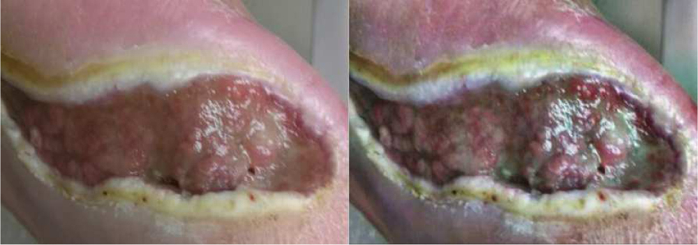
An example image (left) with the Contrast Limited Adaptive Histogram Equalization Image (right)

C. Associative Hierarchical Random Field (AHRF)

Image segmentation using AHRF, a variant of CRF, consists of two parts: 1) calculating the energy value for an image given its pixel-wise labels, which considers both local features and similar neighboring pixels, 2) a graph solving approach, which tries to determine the optimal assignment of labels to an image such that its energy function is minimized. The mathematical formulation of AHRF is explained below. A high-level workflow of AHRF is also shown in Fig-4

Fig. 4:

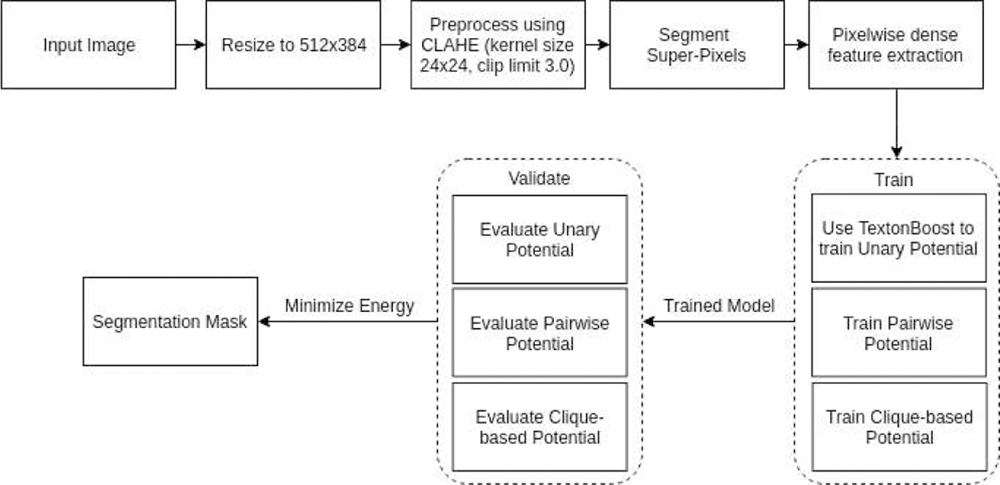
AHRF implementation and workflow

Formulation:

Let us first define the following variables -

X = {X₁, X₂, …X_n} are the variables to be labelled

L = set of labels from which X_i are labeled

y_i = individual label given to X_i such that y_i ∈ L

M = number of paired training instances of the form ${\left\{x^{\left(i\right)},y^{\left(i\right)}\right\}}_{i=1}^M$

V = {1, 2, …n} set of valid vertices or indices of X

N = defined by sets N_i∀i ∈ V where N_i denotes the set of all neighbors of X_i

C = set of all cliques c where a clique X_c is a set of variables X that are similar and codependent such as super-pixels

y_c = labelling given to each clique c

Using the variables defined above, an AHRF formulation consists of an energy function E which is written as the sum of unary, pairwise and clique-wise potential as shown in equation 1 below.

$$E\left(y\right)=\underset{\text{Unary}\hspace{0.17em}\text{Potential}}{\underbrace{\sum _{i\in V}{\varphi }_i\left(y_i,{\theta }_u\right)}}+\underset{\text{Pairwise}\hspace{0.17em}\text{potential}}{\underbrace{\sum _{i\in V,j\in N_i}{\varphi }_{ij}^p\left(y_i,y_j,{\theta }_p\right)}}+\underset{\text{Higher}\hspace{0.17em}\text{order}\hspace{0.17em}\text{Potential}}{\underbrace{\sum _{c\in C}{\varphi }_c^h\left(y_c\right)}}$$ (1)

In the above formulation, θ_u and θ_p are a set of parameters that are learned from the training paired samples ${\left\{x^{\left(i\right)},y^{\left(i\right)}\right\}}_{i=1}^M$ with the objective of maximizing the conditional distribution P (y|X). The higher order potential is described in equation 2 below.

$${\varphi }_c^h(y_c)={\min }_{i\in L}({\gamma }_c^{\max },{\gamma }_c^l+\sum _{i\in c}{w}_i{k}_c^l\Delta (y_i\ne l))$$ (2)

where w_i is the weight of the variable x_i and each variable of a clique is penalized with a cost $w_i{k}_c^l$ if it has not taken the value of the dominant label of that clique. The value of penalty is truncated at ${\gamma }_c^{\max }$. This formulation also supports higher order super-pixel based potentials across multiple scales of the image since it allows for cliques to take a free label in the case of multiple dominant labels and also considers relationships between cliques to increase contextual awareness. We have used mean shift segmentation to generate superpixels. Several different features have been used to calculate the AHRF potentials including textonBoost features on RGB and LAB colorspace, local binary patterns, Histogram of Oriented Gradients (HOG), SIFT features and color distribution features. Given the potential terms and parameters, the optimal labeling can be found by minimizing the overall energy using graph-cut based move making algorithms such as alpha expansion or alpha-beta-swap algorithm.

D. Semantic Segmentation Architectures using CNNs

1). Fully Convolutional Networks (FCNS):

FCNs differ from the classic CNNs used for image classification tasks. The CNN pipeline for image classification usually has a structure with several convolution layers followed by fully connected layers and outputs one predicted label per image. On the other hand, Long et al describe a Fully Connected Network (FCN) as one that uses only convolutions, pooling and activation functions and computes a nonlinear filter [10]. It achieved state-of-the-art segmentation on PASCAL VOC 2012 [30], NYUDv2 and SIFT Flow in 2015.

Classification networks can be converted into FCNs by eliminating the final classifier layers and appending a 1x1 convolution layer with a channel dimension equal to the number of classes to be predicted. This also allows the network to accept arbitrary sized images as input. This modification performs well on segmentation tasks but the output is coarse, which is remedied by adding skips that combine outputs from the lower layers with finer strides to generate the final prediction. This refines the output as local information from the lower layers makes the model pay attention to the global structure. Upsampling is required to fuse these outputs, which is done by deconvolution layers.

Network Structure:

We utilized ResNet101 [16] as the backbone of this network. The model consists of four layers followed by a classifier that segments the pixels into their respective classes. The four layers contain 3, 4, 23 and 3 bottleneck units respectively where each bottleneck consists of four convolution layers that are followed by a batch normalization step. The ReLU activation function is used after each bottleneck.

The third convolution layer in the bottleneck is a 3x3 convolutional operation while the rest are 1x1 convolutions. After the second layer, the bottleneck layers have an added dilation factor in the 3x3 convolutions for improving performance. The classifier consists of a 3x3 convolution followed by batch normalization and ReLU with dropout steps, ending with a 1x1 convolution with a channel dimension equal to the number of output classes.

2). U-Net:

U-Net is a Convolutional Neural Network (CNN) encoder-decoder segmentation architecture proposed by Ronneberger et al [11]. It won the ISBI cell tracking challenge in 2015 and has since been found to perform well on diverse applications of segmentation to medical images. U-Net moves and analyzes a sliding window over a large image, which enables the network to learn contextual information about the image. In our wound segmentation task, this is useful as the network needs to learn the context of skin and discover wound segments inside it. Based on fully convolutional neural networks, U-Net takes advantage of high resolution features from the convolution layers to learn the optimal up-sampling of the image.

Network Structure:

The contracting path consists of 5 down convolution blocks. Each block consists of 3x3 convolution operation with ReLU activation and a 2x2 maxpooling. The U-Net architecture was slightly modified by adding batch-normalization layer after the convolution layer in order to normalize the activations. A dropout layer was also added at the end of each block to prevent over-fitting.

In the expanding path, the transpose convolution operation is utilized for upsampling. The convolution operation is the sum of the dot product of all the values in the kernel and the patch of the image. Transpose convolution does exactly the opposite by taking in single values from the feature map and multiplying them by all values of the learned kernel. This helps in fine-grained up-sampling of the feature map. To facilitate the up-sampling operation, features from the convolution layers are concatenated to the feature map obtained from the last layer. As the contracting and expanding paths are symmetric, a U-shape is formed (as seen in Fig-6), from which the architecture gets its name.

Fig. 6:

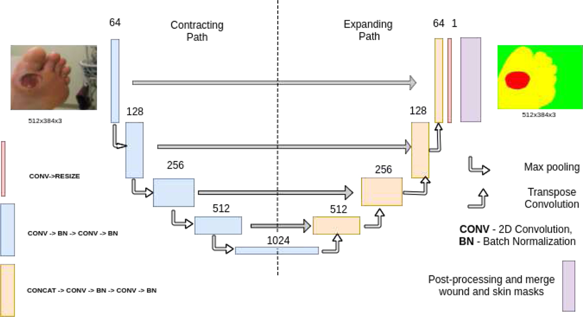
Architecture of U-Net.

3). DeepLabV3:

DeepLabV3 is a convolutional neural network, which uses atrous convolutions in either a cascaded or parallel fashion along with atrous spatial pyramid pooling, enabling the network to capture multi-scale context by using different atrous rates. The performance of DeepLabV3 matched that of other state-of-art models on the PASCAL VOC 2012 segmentation benchmark in 2017. In an ordinary convolutional neural network, pooling and striding cause a reduction in the resolution of the feature maps. Usually, deconvolutional layers are used to upsample and recover spatial resolution. Instead, DeepLabV3 uses atrous convolutions [31] that are essentially convolutions with holes, to effectively enlarge the field of view of filters to improve context assimilation without increasing the number of operations and filter parameters.

Atrous Spatial Pyramid Pooling (ASPP) is the main reason for DeepLabV3’s impressive performance. It consists of four parallel atrous convolutions with different rates that are then applied to the feature map. The atrous convolutions in the pyramid are all followed by batch normalization. Global context is also incorporated into the model by applying global average pooling on the final feature map of the network followed by 1x1 convolution and batch normalization steps. This output is then upsampled bi-linearly to the desired spatial dimension.

Network Structure:

This network also uses ResNet101 as its backbone. The first few layers of this model have a structure similar to the FCN with four layers that have 3, 4, 23 and 3 bottleneck units respectively. The classifier that follows starts off with a 1x1 convolution with batch normalization and a ReLU activation function and this output is fed into the ASPP. The convolution operations in the pyramid are 3x3 with different dilation rates. This is followed by adaptive average pooling for global context and four convolution operations with batch normalization and ReLU activation steps. All convolutions are 1x1 except for the penultimate convolution which is a 3x3 operation.

Loss function:

All the networks described above were trained using Binary Cross Entropy (BCE) as the Loss function.

$$BCE=\sum _{i\in N}\left(-g_i*\log p_i\right)$$ (3)

where p_i is the softmax output given by the network, N is image size, g is the ground truth labels g ∈ {0, 1}, p is the predicted label after applying the softmax operation to the output generated by the output layer of the network.

Dice Coefficient Score:

is a common metric for determining the performance of image segmentation methods [32]. It quantifies the overlap of a segmented image with ground truth segmentation labels. In this paper, we use the Dice Coefficient as our evaluation metric to compare segmentation results as it incorporates both precision and accuracy. The Dice Coefficient is defined as follows -

$$dic{e}_{coeff}=\frac{2*\left|p_{bin}\cap g\right|}{\left|p_{bin}\right|+\left|g\right|}$$ (4)

where p_bin is the binary value of the predicted mask after performing a binary threshold on p_i at 0.5. p_bin ∈ {0, 1}.

The final loss function is a weighed sum of BCE and dice_coeff where k is a manually tuned parameter. The BCE loss helps in increasing the confidence of the network to detect true positives whereas the dice loss penalizes the network for wrong positions of the predicted wound. As both are log losses, they are additive.

$$Loss=BCE-k*\log dic{e}_{coeff}$$ (5)

Post-processing:

The segmentation maps predicted by the networks are sometimes discontinuous and often require post-processing. Hence, the outputs are usually post-processed using a Conditional Random Field (CRF) with Gaussian edge potentials for improving segmentation accuracy [33]. A CRF is characterized by a Gibbs distribution and the Gibbs energy of the graph G = (V, E) is defined in 1 without the higher order term.

For our implementation, the unary potential is defined as the negative log of the softmax output of the network. Thus when the output of the network for a given pixel is close to 1, the unary potential for the corresponding graph node is 0, whereas if the output is close to 0, the unary potential goes to infinity. As the unary and pairwise potentials are calculated independently, the labels predicted by the unary potential alone are significantly affected by noise. A pair-wise potential is devised to incorporate the association between neighboring pixels. The pairwise kernel is defined as in equation 6.

$${\varphi }_{i,j}^p\left(x_i,x_j\right)={\mu }_p\left(x_i,x_j\right)\sum _{m=1}^K{w}^m{k}^m\left(f_i,f_j\right)$$ (6)

where µ is the Potts model and K(f_i, f_j) are Gaussian

$$k^m\left(f_i,f_j\right)=\underset{\text{appearence}\hspace{0.17em}\text{kernel}}{\underbrace{w^1\exp \left(-\frac{{\left|p_i-p_j\right|}^2}{2{\theta }_{\alpha }^2}-\frac{{\left|I_i-I_j\right|}^2}{2{\theta }_{\beta }^2}\right)}}+\underset{\text{smoothness}\hspace{0.17em}\text{kernel}}{\underbrace{w^2\exp \left(-\frac{{\left|p_i-p_j\right|}^2}{2{\theta }_{\gamma }^2}\right)}}$$ (7)

The appearance kernel associates pixels with similar color and penalizes pixels with large differences in color. It considers both pixel intensities in individual image channels I and their positions p. In our case, the image vector I has [R, G, B] pixel values from the input image, and is parameterized by θ_α and θ_β. The smoothness kernel penalizes only based on the nearness of the pixels and is parameterized by θ_γ.

E. Training the AHRF Model

AHRF uses gradient boosting techniques to optimize the unary potential and graph-cut algorithm to optimize the CRF graph. The Contrast Limited Adaptive Histogram Equalization (CLAHE) [29] pre-processing technique was found to increase the dice score of wound segmentation. Optimal parameters of the CLAHE technique were found using grid search on Dataset 1. The parameters for CLAHE implementation of openCV used in our results are kernel size of 24, 24 and clip limit of 3.0. AHRF was trained on a multi-threaded high performance cluster with 20 CPUs and 100 GB memory. The framework parallelizes feature extraction and utilized up to 40 threads.

F. Training the Semantic Segmentation Networks

All the networks utilize high resolution features from the convolution layers in learning the optimal up-sampling of the image. In our experiments, all images were resized to a standard dimension of 512 x 384 before being input to to the network. As all the images in the dataset were of varying dimensions and aspect ratios, we averaged the dimensions of all images and approximated them to the closest even value required to maintain an aspect ratio of 4:3.

As the number of image samples in our datasets were inadequate for neural networks, a probabilistic data augmentation pipeline was implemented to generate synthetic augmentations using the albumentations library [34]. The augmentations used were geometric in nature including vertical flip, horizontal flip, random rotate, scale and translation. To compensate for various lighting conditions augmentations such as CLAHE, random contrast and blurring were also added to the pipeline. At run time, every augmentation was chosen with a probability p. Only one augmentation from the set CLAHE, random contrast, median blur and random brightness was chosen with a probability p = 0.5 and the rest of the augmentations were chosen with p = 0.5 each. This ensured that CLAHE and blurring, or contrast and blurring were not performed on the same image. Refer: Fig-8.

Fig. 8:

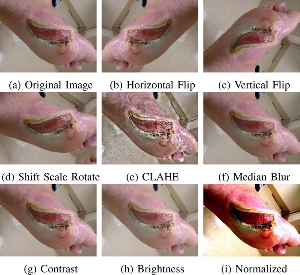
Sample image augmentations done online during training

The FCN and DeepLabV3 models we utilized were pre-trained on a subset of the COCO train2017 dataset, while U-Net was initialized with weights from the Carvana Image Classification Challenge. The networks were then fine-tuned using images from wound datasets using Stochastic Gradient Descent (SGD). FCN and DeepLabV3 were trained for only 50 epochs as their superior initial weights made them converge quickly. U-Net was trained for more epochs [500–600 epochs] with early stopping. Six-fold validation was used to evaluate the generalization of the networks. The models were implemented in PyTorch [35] and its built-in optimizers were used for the training process.

FCN and DeepLabV3 were trained on a High Performance Cluster (HPC) with a Tesla K40 and 2 Intel Xeons and took one day to train all folds. On the other hand, U-Net was trained on an i7 CPU with 32GB memory and a GTX1080Ti GPU and took 5 days to train. Two separate networks were trained for U-Net - one for classifying between wound vs non-wound pixels, and the other for classifying skin vs non-skin pixels. The masks of these two networks are combined at the end to generate a final segmentation mask. All inferences were run on the GTX1080Ti. As the Gaussian edge-based CRF model used for post-processing could not be optimized during back propagation of the network, the θ_α, θ_β, θ_γ parameters were optimized separately using grid search.

G. Evaluation

All semantic segmentation methods were evaluated using k-fold cross validation over the entire dataset with k = 6. Performance of the model on test set is measured by using the Dice Coefficient Score.

V. Results and Discussions

1). Comparing Segmentation Inference Time:

AHRF is a graph optimization method and takes about 3–5 minutes to infer segmentation masks for a single image of size 512x384 on all three datasets (see column 4 of Tables - III to V). Although the graph optimization step is faster, the feature extraction and evaluation steps makes inference in AHRF significantly slow. Consequently, it would be challenging to implement AHRF on mobile devices. CNNs on the other hand utilize a series of matrix multiplications and additions amenable for implementation on GPUs, which most smartphones are equipped with. FCN, U-Net and DeepLabV3 had an average inference time of approximately 41, 50 and 56 milliseconds on all three datasets.

TABLE III:

Results for Dataset 1 (95 Train, 19 Validation)

Model	MAE (mm)	Hausdorff (mm)	Dice Wound	Dice Skin	Inference time
CLAHE + AHRF	0.0904	11.553	0.750	0.9060	3–5 min
U-Net	0.1880	13.983	0.490	0.7950	40 msec
U-Net + CRF	0.1552	13.165	0.520	0.8900	2 sec
CLAHE + U-Net	0.1523	13.085	0.532	0.8901	50 msec
CLAHE + U-Net + CRF	0.1231	12.365	0.591	0.8903	2 sec
FCN	0.0681	10.791	0.7822	0.9410	41 msec
CLAHE + FCN	0.0777	11.136	0.7667	0.9378	51 msec
DeepLabV3	0.0783	11.164	0.7625	0.9352	56 msec
CLAHE + DeepLabV3	0.0811	11.220	0.7595	0.9320	66 msec

TABLE V:

Results for Dataset 3 (1201 Train, 241 Validation)

Model	MAE (mm)	Hausdorff (mm)	Dice Wound	Dice Skin	Inference time
CLAHE + AHRF	0.1235	12.377	0.6287	0.9016	3–5 min
U-Net	0.0832	11.372	0.733	0.9506	40 msec
U-Net + CRF	0.0830	11.369	0.734	0.9506	2 sec
CLAHE + U-Net	0.0875	11.479	0.7200	0.9474	50 msec
CLAHE + U-Net + CRF	0.0878	11.486	0.719	0.9473	2 sec
FCN	0.0464	10.092	0.8518	0.9532	41 msec
CLAHE + FCN	0.0559	10.878	0.8357	0.9518	51 msec
DeepLabV3	0.0379	9.764	0.8554	0.9617	56 msec
CLAHE + DeepLabV3	0.0534	10.631	0.8390	0.9578	66 msec

2). Comparing Segmentation Accuracy:

Dataset 1:

As observed in Table-III, AHRF is significantly more accurate than U-Net by a difference of 0.159 dice score on the wound segments in dataset 1. Both Pre-processing (CLAHE) and Post-processing (CRF) improve the performance of the segmentation of U-Net. However, even with these pre- and post-processing techniques, U-Net is not as accurate as AHRF. On the other hand, FCN and DeepLabV3 both outperform AHRF even with less data, which can be attributed to the models being trained on a subset of COCO train2017 and then fine-tuned to our dataset. FCN outperforms DeepLabV3 by 0.0197 in dice score which is because FCN is a lighter model and hence, fits the data distribution slightly better than DeepLabV3. FCN and DeepLabV3 outperforms AHRF by dice scores of 0.0322 and 0.0125 respectively.

Dataset 2:

As the dataset size increases, the networks generalize to the distinct features and textures that define a wound. As seen in Table-IV, U-Net has a slightly higher dice score than AHRF (more accurate). Pre-processing U-Net using CLAHE improved its accuracy but the improvement observed is less than that obtained for Dataset 1 but it underperforms FCN and DeepLabV3 again, with a difference of 0.124 and 0.122 in dice score respectively. Ultimately, as the size of the training data increases, U-Net’s dependence on pre- and post- processing decreases as it learns better features. The performance of FCN and DeepLabV3 is not affected by pre- and post- processing due to their pre-trained weights and model architectures (DeepLabV3). FCN and DeepLabV3 outperformed AHRF by dice scores of 0.135 and 0.133 respectively.

TABLE IV:

Results for Dataset 2 (263 Train, 53 Validation)

Model	MAE (mm)	Hausdorff (mm)	Dice Wound	Dice Skin	Inference time
CLAHE + AHRF	0.1072	11.969	0.706	0.8865	3–5 min
U-Net	0.1152	12.169	0.665	0.897	40 msec
U-Net + CRF	0.1147	12.156	0.667	0.897	2 sec
CLAHE + U-Net	0.1028	11.861	0.717	0.892	50 msec
CLAHE + U-Net + CRF	0.1023	11.848	0.716	0.895	2 sec
FCN	0.0645	10.907	0.8418	0.9342	41 msec
CLAHE + FCN	0.0744	11.356	0.8220	0.9262	51 msec
DeepLabV3	0.0662	10.949	0.8392	0.9330	56 msec
CLAHE + DeepLabV3	0.0720	11.318	0.8268	0.9278	66 msec

Dataset 3:

The third dataset containing 1442 images is roughly four times the size of dataset 2. Even though it has more variance (see Table -I, Table-II), the CNNs generalize to all types of wounds and generate segmentation masks close to the ground truth, whereas the performance of AHRF decreases slightly. As observed in Fig-13 - sample 1, AHRF tends to get confused for the same image as the variations in the dataset increases, making it less robust. The CNNs also generate better segmentation masks for smaller wounds as seen in Fig-9-sample 4. U-Net has a significantly higher dice score than AHRF with a margin of 0.106 dice co-efficient and does not require any pre/post-processing. AHRF is observed to over-segment and often performs poorly on edges and wounds with difficult textures. FCN and DeepLabV3 still outperform U-Net by a dice score of 0.117 and 0.121 respectively, which highlights the impact of using pre-trained models. DeepLabV3, a deeper model, outperforms FCN as dataset 3 has significantly more data for it to work with.

Fig. 13:

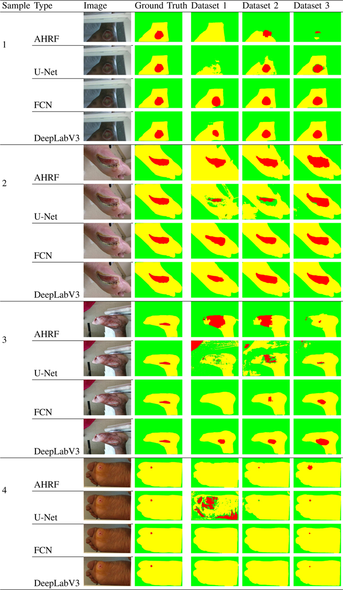
Comparison of AHRF, U-Net, FCN, DeepLabV3 and their accuracy trends on all 3 datasets. Sample 1 shows how the accuracy of AHRF improves from Dataset 1 to Dataset 2 but then decreases when more, noisier data is added in Dataset 3. The deep learning networks on the other hand shows consistent improvement as more data is added. The samples demonstrate how skin pixels are segmented more accurately than the wound segment because of the huge class imbalance in data.

Fig. 9:

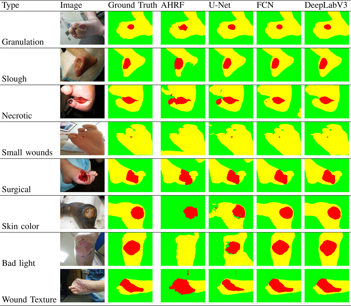
Performance of AHRF, U-Net, FCN and DeepLabV3 trained on Dataset 3 for segmenting a variety of images with different colors, textures and lighting conditions of skin, wound and background

a). Common validation dataset: :

In order to get a final conclusion on the accuracy of all the segmentation methods, we compared their segmentation accuracy on a common validation set after being trained on datasets 1, 2 and 3 respectively (see Table-VI) It can be concluded from this table that the accuracy of deep learning models increases with increase in the data samples while the performance remains same or sometimes worsens for AHRF, a graph based segmentation architecture.

TABLE VI:

Common Validation Set - WOUND

Model	Dataset 1	Dataset 2	Dataset 3
AHRF	0.673	0.687	0.675
U-Net	0.416	0.717	0.784
FCN	0.7822	0.8453	0.859
DeepLabV3	0.7625	0.8537	0.876

Average dice coefficients for common images in all 3 datasets.

3). Model Robustness to wound colors in background:

In many wound imaging situations, colors found in many wounds such as red and yellow may appear in the background by accident. Thus, it is important to compare how robust (i.e. does not detect those background colors as part of the wound) the segmentation methods are when such colors appear in the background. Since the networks are pre-trained and are being fine-tuned on the wound segmentation task, the network tries to learn the most prominent features of the wound at first. It can be clearly observed in Fig-13 - sample 3, dataset 1, that U-Net initially (on smaller datasets) tends to classify any red color in the wound image as belonging to the wound segment. This can be justified from Table-II which shows that the mean value of the Red channel of the wound segment of dataset 1 is higher than the Blue and Green channels. However, as U-Net is trained on more data, it starts to learn and rely on texture information as well. This can be seen in Fig-13 sample 3, where U-Net does not confuse the red cloth in the top left corner with the wound when trained on dataset 3. FCN and DeepLabV3 do not face this issue as they utilize pre-trained weights, alleviating their dependence on just color. AHRF on the other hand uses hand-crafted features, is more robust to wound colors in the background. It requires fewer images to achieve its performance limits and thus does not confuse the red cloth with the wound irrespective of which dataset it has been trained on. This shows that handcrafted features help AHRF understand textures better than U-Net when trained on smaller datasets but due to information contained in their initial weights, FCN and DeepLabV3 already take textures into consideration.

4). Effect of class imbalance:

We compared the accuracy of the CNNs and AHRF for wound images with varying sizes of wound and skin segments. It can be observed in Sample 4 of Fig-9 how detection of skin pixels (larger segments) is better than that of the wound segment (smaller) for the networks because of the huge class imbalance in data. This trend is not observed for AHRF because AHRF is trained jointly for all three classes. Hence, the wound classifier can utilize the information learned for skin. For example, areas not classified as skin but surrounded by skin automatically get a higher probability of belonging to the wound class.

5). Sensitivity to the Relative Proportion of the Wound Segment:

The sensitivity of segmentation to changes in the proportion of image covered by the wound is studied for all three datasets. Figures 10, 11, and 12 show the accuracy of AHRF and the CNNs as the wound size varies in the form of box plots. We show box plots that includes information on both the mean Dice score as well as its variation across various folds. The width of the box plot shows how stable the reported mean Dice score is across various folds. Dice score variance is shown for percentage of wound pixels in the images. The wound percentage is defined as the ratio of number of wound pixels to the total number of pixels. Due to the connective property of AHRF which results from its clique potential, it fails to work well on images that have small wounds because neighboring skin pixels cause a small wound to also be classified as skin. The deep learning networks do not face this problem and work well on wounds of a small size.

Fig. 10:

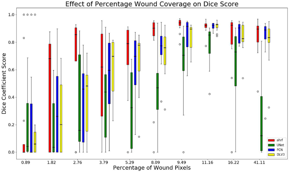
Box plots of wound percentage of wound pixels vs dice coefficient for dataset 1

Fig. 11:

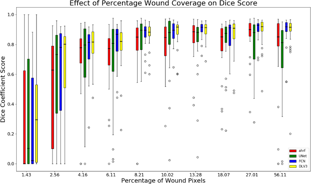
Box plots of wound percentage of wound pixels vs dice coefficient for dataset 2

Fig. 12:

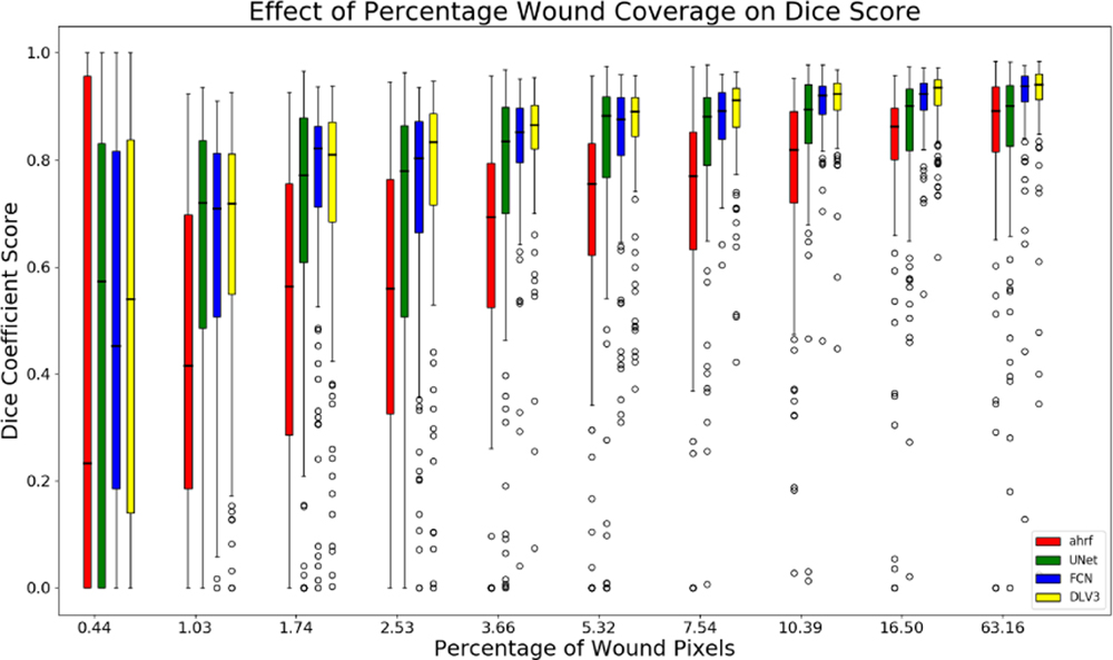
Box plots of wound percentage of wound pixels vs dice coefficient for dataset 3

The box-plot in Fig-10 shows that AHRF performs better than U-Net even with large variations in the wound size for dataset 1 while FCN and DeepLabV3 match its performance. The CNNs fail to detect wounds smaller than 10% of the wound image whereas AHRF generates some slight segmentations. The box-plot in Fig-11 and Fig-12 shows increased accuracy with as wound size increases for datasets 2 and 3. The height of the boxes shows variance in the performance of all architectures. It can be observed that images with more than 5% of wound pixels have better results for all the architectures. This result can be used to create a guideline for taking usable wound images or cropping the images in a pre-processing phase by keeping the wound percentage more than 5%. For instance, the photographer can be asked to retake (or zoom in) images in which the wound percentage is less than 5%.

6). Segmentation Accuracy for wounds with different wound attributes and skin types:

As seen in Fig-9, both AHRF and the CNNS have shown good generalizability to various wound tissue types, skin colors and lighting conditions. Granulation, slough and necrotic are different types of wound tissue which occur in wounds, which differ in their color and texture. However, both AHRF and the networks have shown good segmentation results on wounds containing a combination of these tissues. The networks generalize well to darker skin tones and bad lighting conditions as well.

VI. Discussions and Conclusion

In this work, a comprehensive systematic analysis of semantic segmentation of smartphone camera captured wound images using AHRF, FCN, U-Net and DeepLabV3 has been performed. All segmentation methods achieve good results which generalize well in wound images with various skin and wound tissue types, and background clutter. However, due to differences in the two approaches (AHRF vs deep learning), some trade-offs have to be considered before deciding on a model for practical purposes.

AHRF had increased segmentation accuracy when input images were pre-processed using CLAHE.

CLAHE pre-processing with U-Net showed improvements only for smaller datasets. CRF post-processing also improved the accuracy of U-Net on smaller datasets. Pre- and post-processing did not change the performance of FCN and DeepLabV3.

AHRF is more accurate and generalizes better than U-Net for small datasets (< 300 images) but is outperformed by fine-tuned FCN and DeepLabV3 models pre-trained on PASACL VOC:

AHRF has more reliable predictions because it depends on texture features and not just color. Its hand-crafted visual features also enable it to learn wound features with fewer images. U-Net on the other hand, performed moderately well for segmenting skin but not wound pixels on Dataset 1 (smallest dataset). FCN and DeepLabV3 performed well in segmenting both skin and wound pixels across all 3 datasets.

CNNs are more accurate for larger datasets (> 300 images).

As the size of dataset increases, the segmentation accuracy of the deep learning networks increase while that of AHRF saturates after a point and sometimes even worsens with the addition of more training data. As FCN, U-Net and DeepLabV3 have many more trainable hyperparameters than AHRF, they are able to absorb and utilize more data and generalize better. They also show better performance on smaller wound sizes as compared to AHRF. This is because AHRF has a region growing property due to its pairwise and clique potentials which causes smaller wounds to sometimes become part of the surrounding skin clique which are wrongly segmented as skin.

CNNs have a considerably faster inference time than AHRF:

mainly because AHRF uses many hand-crafted features and clustering techniques, which take time to be computed. In our experiments, AHRF took about 4–5 minutes for segmenting one image while FCN, U-Net and DeepLabV3 could segment the same image in about 40, 50, 60 milliseconds respectively. This makes the networks a more viable option for implementation on mobile devices, where resources are constrained, especially if real-time segmentation is required. The long inference time of AHRF makes it difficult to use even in a client-server scenario, as a network connection would probably timeout before segmentation is complete.

Initial weights of deep learning approaches make a considerable difference:

U-Net generally outperforms FCNs, but FCN outperforms U-Net in our experiments by a margin 0.075 for dataset 3 as seen in Table-VI. FCN and DeeplabV3 were initialized with pre-trained weights from COCO train2017 while U-Net was initialized with weights from the Carvana Image Classification Challenge. Using these weights for U-Net was better than using random initialization but are still no match for COCO train2017 weights. DeepLabV3 outperformed FCN by a margin of 0.017 for dataset 3 in Table-VI.

VII. Future Work

One possible future direction for this research could be experimenting more with lighting variations and performing an error analysis of the various factors which affect the segmentation performance of AHRF and the deep learning models. Models can be made more robust by using Generative Adversarial Networks (GANs)[36] for synthesizing more training data. More effective ways of image pre-processing such as auto-augmentation [37] can also be used which trains a neural network to decide on the best possible pre-processing step for a given input image. Finally, parallelizing AHRF to make it faster, especially the feature extraction might be a fruitful direction for further research.

Fig. 1:

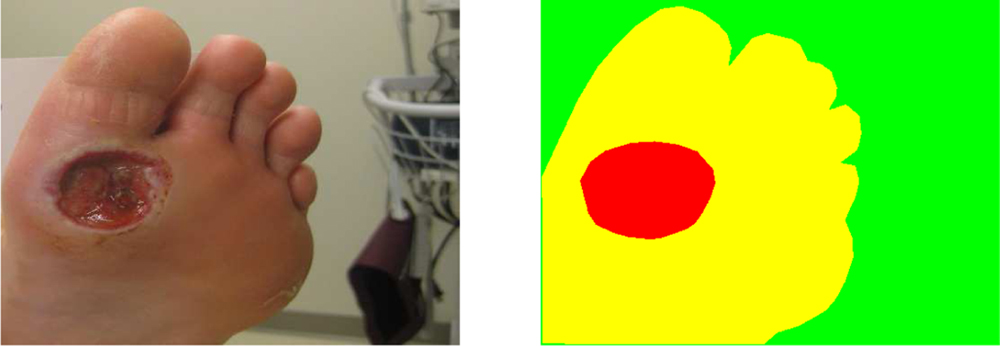
Wound image (left), pixel-wise segmentation mask for wound, skin and background (right)

Fig. 5:

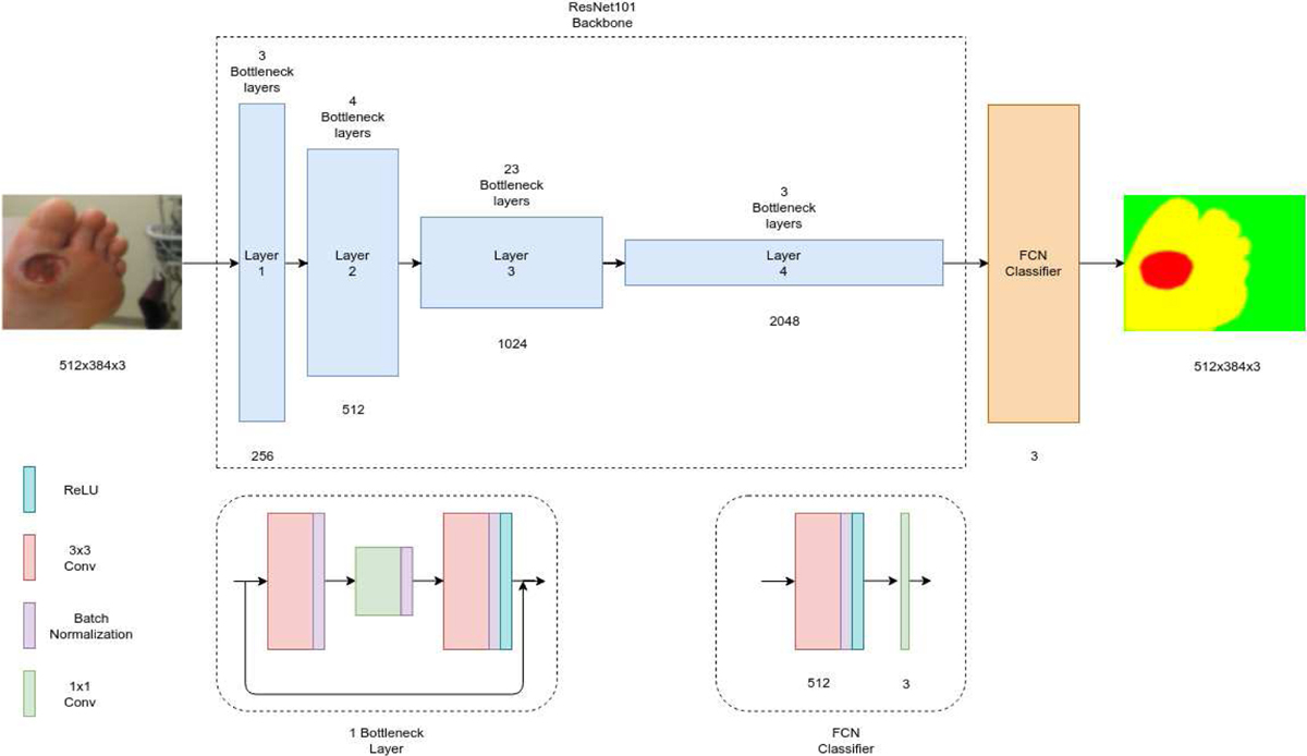
Architecture of FCN.

Fig. 7:

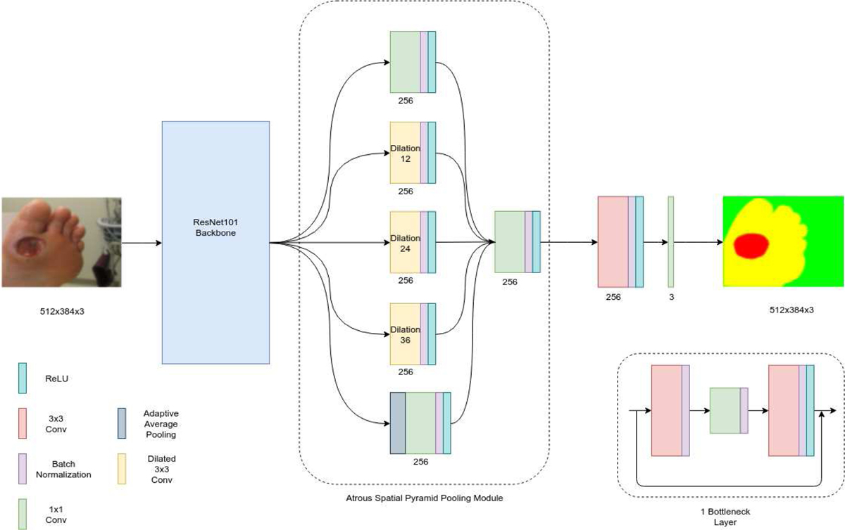
Architecture of DeepLabV3.

Biographies

Shubham Jain received the B.Tech Degree from the Indian Institute of Technology Kanpur, India in 2017 and M.S. degree in robotics engineering from the Worcester Polytechnic Institute, Worcester, MA, USA, in 2019. He currently works as a Computer Vision Engineer with NVIDIA. His current research interests include autonomous driving and related computer vision problems

Ameya Wagh received the M.S. degree in robotics engineering from the Worcester Polytechnic Institute, Worcester, MA, USA, in 2019. He currently works as a Software Engineer with TORC Robotics. His current research interests include computer vision and deep learning.

Apratim Mukherjee is currently pursuing his Bachelor’s degree in Computer Science and Engineering from Manipal Institute of Technology, India and will graduate in the summer of 2020. His research interests lie in the fields of robotics and computer vision.

Ziyang Liu is currently pursuing the Ph.D. degree in computer science with the Worcester Polytechnic Institute, MA, USA. His current research interests include computer vision and deep learning.

Emmanuel Agu received the Ph.D. degree in electrical and computer engineering from the University of Massachusetts Amherst, Amherst, MA, USA, in 2001. He is currently a Professor with the Computer Science Department, Worcester Polytechnic Institute, Worcester, MA, USA. He has been involved in research in mobile and ubiquitous computing for over 16 years. He is currently working on mobile health projects to assist patients with diabetes, obesity, and depression.

Peder C. Pedersen (S’74–M’76–SM’87) received the B.S. degree in electrical engineering from Aalborg Engineering College, Aalborg, Denmark, in 1971, and the M.E. and Ph.D. degrees in bioengineering from the University of Utah, Salt Lake City, UT, USA, in 1974 and 1976, respectively. In October 1987, he joined the faculty at Worcester Polytechnic Institute, Worcester, MA, USA, where he is now an emeritus Professor in the Electrical and Computer Engineering Department. Previously, he was an Associate Professor in the Department of Electrical and Computer Engineering, Drexel University, Philadelphia, PA. His research areas include elastography methods for quantitative imaging of the Young’s modulus in soft tissues and the development of a low-cost, portable personal ultrasound training simulator with structured curriculum and integrated assessment methods, to satisfy the training needs of the widely used point-of-care scanners. Another research effort has been the design of a smartphone-based diabetic wound analysis system, specifically for foot ulcers.

Diane Strong received the B.S. degree in mathematics and computer science from the University of South Dakota, Vermillion, SD, USA, in 1974, the M.S. degree in computer and information science from the New Jersey Institute of Technology, Newark, NJ, USA, in 1978, and the Ph.D. degree in information systems from the Tepper School of Business, Carnegie Mellon University, Pittsburgh, PA, USA, in 1989. Since 1995, she has been a Professor with the Worcester Polytechnic Institute, Worcester, MA, USA, where she is currently a Full Professor with the Foisie School of Business and also the Director of Information Technology Programs. She is also a member of the Faculty Steering Committee of WPI’s Healthcare Delivery Institute. Her research has been concerned with effective use of IT in organizations and by individuals. Since 2006, she has focused on effectively using IT to promote health and support healthcare delivery.

Bengisu Tulu received the Ph.D. degree in management of information systems and technology from Claremont Graduate University, CA, USA. She is currently an Associate Professor with the Foisie Business School, Worcester Polytechnic Institute, Worcester, MA, USA. She is one of the founding members of the Healthcare Delivery Institute, WPI. Her research interest includes development and implementation of health information technologies and the impact of these implementations on healthcare organizations and consumers.

Clifford Lindsay received the B.S. degree in computer science from the University of California, San Diego, San Diego, CA, USA, in 2001, and the Ph.D. degree in computer science from the Worcester Polytechnic Institute, Worcester, MA, USA, in 2011. He is currently an Assistant Professor with the UMass Medical School. He is also working on applying computer vision and image processing methods to improve the quality of medical images.

REFERENCES

- [1].Beck J, Greenwood DA, Blanton L, Bollinger ST, Butcher MK, Condon JE, Cypress M, Faulkner P, Fischl AH, Francis T, Kolb LE, Lavin-Tompkins JM, MacLeod J, Maryniuk M, Mensing C, Orzeck EA, Pope DD, Pulizzi JL, Reed AA, Rhinehart AS, Siminerio L, and Wang J, “2017 National Standards for Diabetes Self-Management Education and Support,” Diabetes Educator, vol. 44, no. 1, pp. 35–50, 2018. [DOI] [PubMed] [Google Scholar]
- [2].Sen CK, Gordillo GM, Roy S, Kirsner R, Lambert L, Hunt TK, Gottrup F, Gurtner GC, and Longaker MT, “Human skin wounds: A major and snowballing threat to public health and the economy,” Wound Repair and Regeneration, vol. 17, pp. 763–771, 2009. [DOI] [PMC free article] [PubMed] [Google Scholar]
- [3].Houghton PE, Kincaid CB, Campbell KE, Woodbury MG, and Keast DH, “Photographic assessment of the appearance of chronic pressure and leg ulcers.” Ostomy/wound management, vol. 46, no. 4, pp. 20–6, 28–30, 2000. [PubMed] [Google Scholar]
- [4].Murphy CA, Houghton P, Brandys T, Rose G, and Bryant D, “The effect of 22.5 kHz low-frequency contact ultrasound debridement (LFCUD) on lower extremity wound healing for a vascular surgery population: A randomised controlled trial,” International Wound Journal, vol. 15, no. 3, pp. 460–472, 2018. [DOI] [PMC free article] [PubMed] [Google Scholar]
- [5].Haugland H, Hisdal J, Sundby ØH, Lundgaard E, Irgens I, Sandbæk G, Høiseth LØ, Weedon-Fekjær H, Mathiesen I, and Sundhagen JO, “Intermittent mild negative pressure applied to the lower limb in patients with spinal cord injury and chronic lower limb ulcers: a crossover pilot study,” Spinal Cord, vol. 56, no. 4, pp. 372–381, 2018. [DOI] [PubMed] [Google Scholar]
- [6].Sheehan P, Jones P, Caselli A, Giurini JM, and Veves A, “Percent change in wound area of diabetic foot ulcers over a 4-week period is a robust predictor of complete healing in a 12-week prospective trial,” Diabetes Care, vol. 26, no. 6, pp. 1879–1882, 2003. [DOI] [PubMed] [Google Scholar]
- [7].Krizhevsky A and Hinton GE, “ImageNet Classification with Deep Convolutional Neural Networks,” Neural Information Processing Systems, 2012. [Google Scholar]
- [8].Chen L-C, Papandreou G, Schroff F, and Adam H, “Rethinking Atrous Convolution for Semantic Image Segmentation,” arXiv e-prints, June 2017. [Google Scholar]
- [9].Girshick R, “Fast R-CNN,” Proceedings of the IEEE International Conference on Computer Vision, vol. 2015 Inter, pp. 1440–1448, 2015. [Google Scholar]
- [10].Long J, Shelhamer E, and Darrell T, “Fully convolutional networks for semantic segmentation,” in The IEEE Conference on Computer Vision and Pattern Recognition (CVPR), June 2015. [DOI] [PubMed] [Google Scholar]
- [11].Ronneberger O, Fischer P, and Brox T, “U-net: Convolutional networks for biomedical image segmentation,” Lecture Notes in Computer Science (including subseries Lecture Notes in Artificial Intelligence and Lecture Notes in Bioinformatics), vol. 9351, pp. 234–241, 2015. [Google Scholar]
- [12].Shenoy V, Foster E, Aalami L, Majeed B, and Aalami O, “Deep-wound: Automated Postoperative Wound Assessment and Surgical Site Surveillance through Convolutional Neural Networks,” July 2018. [Google Scholar]
- [13].Goyal M, Reeves ND, Davison AK, Rajbhandari S, Spragg J, and Yap MH, “DFUNet: Convolutional Neural Networks for Diabetic Foot Ulcer Classification,” IEEE Transactions on Emerging Topics in Computational Intelligence, pp. 1–12, 2018. [Google Scholar]
- [14].Lin T-Y, Maire M, Belongie SJ, Bourdev LD, Girshick RB, Hays J, Perona P, Ramanan D, Dollár P, and Zitnick CL, “Microsoft coco: Common objects in context,” in ECCV, 2014. [Google Scholar]
- [15].Ladický L, Russell C, Kohli P, and Torr PH, “Associative hierarchical random fields,” IEEE Transactions on Pattern Analysis and Machine Intelligence, vol. 36, no. 6, pp. 1056–1077, 2014. [DOI] [PubMed] [Google Scholar]
- [16].He K, Zhang X, Ren S, and Sun J, “Deep Residual Learning for Image Recognition,” arXiv e-prints, December 2015. [Google Scholar]
- [17].Perez AA, Gonzaga A, and Alves JM, “Segmentation and analysis of leg ulcers color images,” in Proceedings - International Workshop on Medical Imaging and Augmented Reality, MIAR 2001, 2001. [Google Scholar]
- [18].M. R., M. D.D., D. D.K., A. A., M. A., and C. C., “Automated tissue classification framework for reproducible chronic wound assessment,” BioMed Research International, vol. 2014, 2014. [DOI] [PMC free article] [PubMed] [Google Scholar]
- [19].Wang L, Pedersen PC, Agu E, Strong DM, and Tulu B, “Area Determination of Diabetic Foot Ulcer Images Using a Cascaded Two-Stage SVM-Based Classification,” IEEE Transactions on Biomedical Engineering, vol. 64, no. 9, pp. 2098–2109, 2017. [DOI] [PubMed] [Google Scholar]
- [20].Yadav MK, Manohar DD, Mukherjee G, and Chakraborty C, “Segmentation of Chronic Wound Areas by Clustering Techniques Using Selected Color Space,” Journal of Medical Imaging and Health Informatics, 2013. [Google Scholar]
- [21].Shih H-F, Ho T-W, Hsu J-T, Chang C-C, Lai F, and Wu J-M, “Surgical wound segmentation based on adaptive threshold edge detection and genetic algorithm,” Proceedings of the Spie, vol. 225, no. February 2017, February 2017. [Google Scholar]
- [22].Goyal M, Reeves ND, Rajbhandari S, Spragg J, and Yap MH, “Fully convolutional networks for diabetic foot ulcer segmentation,” 2017 IEEE International Conference on Systems, Man, and Cybernetics, SMC 2017, vol. 2017-Janua, pp. 618–623, 2017. [Google Scholar]
- [23].Liu X, Wang C, Li F, Zhao X, Zhu E, and Peng Y, “A framework of wound segmentation based on deep convolutional networks,” Proceedings - 2017 10th International Congress on Image and Signal Processing, BioMedical Engineering and Informatics, CISP-BMEI 2017, vol. 2018-Janua, no. 0800067314001, pp. 1–7, 2018. [Google Scholar]
- [24].Goyal M, Reeves N, Rajbhandari S, and Yap MH, “Robust Methods for Real-time Diabetic Foot Ulcer Detection and Localization on Mobile Devices,” IEEE Journal of Biomedical and Health Informatics, pp. 1–12, 2018. [DOI] [PubMed] [Google Scholar]
- [25].Li F, Wang C, Liu X, Peng Y, and Jin S, “A Composite Model of Wound Segmentation Based on Traditional Methods and Deep Neural Networks,” Computational Intelligence and Neuroscience, vol. 2018, no. 1, 2018. [DOI] [PMC free article] [PubMed] [Google Scholar]
- [26].Maninis K-K, Caelles S, Pont-Tuset J, and Van Gool L, “Deep extreme cut: From extreme points to object segmentation,” in Proceedings of the IEEE Conference on Computer Vision and Pattern Recognition, 2018, pp. 616–625. [Google Scholar]
- [27].Wang L, Pedersen PC, Strong DM, Tulu B, Agu E, and Ignotz R, “Smartphone-based wound assessment system for patients with diabetes,” IEEE Transactions on Biomedical Engineering, 2015. [DOI] [PubMed] [Google Scholar]
- [28].Zuiderveld K, “Contrast Limited Adaptive Histogram Equalization,” in Graphics Gems, 1994. [Google Scholar]
- [29].Pizer SM, Amburn EP, Austin JD, Cromartie R, Geselowitz A, Greer T, ter Haar Romeny B, Zimmerman JB, and Zuiderveld K, “Adaptive histogram equalization and its variations,” Computer Vision, Graphics, and Image Processing, 1987. [Google Scholar]
- [30].Everingham M, Van Gool L, Williams CKI, Winn J, and Zisserman A, “The pascal visual object classes (voc) challenge,” International Journal of Computer Vision, vol. 88, no. 2, pp. 303–338, June 2010. [Google Scholar]
- [31].Chen L-C, Papandreou G, Kokkinos I, Murphy K, and Yuille AL, “DeepLab: Semantic Image Segmentation with Deep Convolutional Nets, Atrous Convolution, and Fully Connected CRFs,” arXiv e-prints, June 2016. [DOI] [PubMed] [Google Scholar]
- [32].Dice LR, “Measures of the Amount of Ecologic Association Between Species,” Ecology, 2006. [Google Scholar]
- [33].Krähenbühl P and Koltun V, “Efficient Inference in Fully Connected CRFs with Gaussian Edge Potentials,” pp. 1–9, 2012. [Google Scholar]
- [34].Buslaev A, Parinov A, Khvedchenya E, Iglovikov VI, and Kalinin AA, “Albumentations: fast and flexible image augmentations,” 2018. [Google Scholar]
- [35].Paszke A, Chanan G, Lin Z, Gross S, Yang E, Antiga L, and Devito Z, “Automatic differentiation in PyTorch,” 31st Conference on Neural Information Processing Systems, no. Nips, pp. 1–4, 2017. [Google Scholar]
- [36].Radford A, Metz L, and Chintala S, “Unsupervised Representation Learning with Deep Convolutional Generative Adversarial Networks,” pp. 1–16, 2015. [Google Scholar]
- [37].Cubuk ED, Zoph B, Mane D, Vasudevan V, and Le QV, “AutoAugment: Learning Augmentation Policies from Data,” 2018. [Google Scholar]