Data analysis of Covid-19 pandemic and short-term cumulative case forecasting using machine learning time series methods

Highlights

• •The cumulative coronavirus cases for USA, Germany and Global are forecasted.
• •Four different machine learning time series methods are employed.
• •SVM method achieves the best trend.
• •Largest extreme value distribution fits best for Covid-19 global cumulative weekly cases.

Abstract

The Covid-19 pandemic is the most important health disaster that has surrounded the world for the past eight months. There is no clear date yet on when it will end. As of 18 September 2020, more than 31 million people have been infected worldwide. Predicting the Covid-19 trend has become a challenging issue. In this study, data of COVID-19 between 20/01/2020 and 18/09/2020 for USA, Germany and the global was obtained from World Health Organization. Dataset consist of weekly confirmed cases and weekly cumulative confirmed cases for 35 weeks. Then the distribution of the data was examined using the most up-to-date Covid-19 weekly case data and its parameters were obtained according to the statistical distributions. Furthermore, time series prediction model using machine learning was proposed to obtain the curve of disease and forecast the epidemic tendency. Linear regression, multi-layer perceptron, random forest and support vector machines (SVM) machine learning methods were used. The performances of the methods were compared according to the RMSE, APE, MAPE metrics and it was seen that SVM achieved the best trend. According to estimates, the global pandemic will peak at the end of January 2021 and estimated approximately 80 million people will be cumulatively infected.

1. Introduction

The COVID-19 disease, which occurred after December 2019, spread all over the world after February 2020. The virus has passed from animals to humans and is transmitted from person to person via airborne droplets [8]. In a short time, it became the biggest epidemic the world has seen in the last century. With respect to data from World Health Organization (WHO), the number of cases seen worldwide is increasing rapidly. Despite the measures taken, the virus has not yet been stopped because of its high infectious power.

Since COVID-19 first emerged, various trend analysis studies have been conducted. Fanelli and Piazza [6] analyzed the temporal dynamics of the coronavirus disease 2019 outbreak in China, Italy and France. Yesilkanat [20] estimated the near future case numbers for 190 countries in the world using random forest algorithm. Sahin and Sahin [12] estimated the cumulative cases of COVID-19 using fractional nonlinear grey Bernoulli model. Yadav et al. [18] analyzed COVID-19 spread using machine learning methods. Kaxiras et al. [9] used Susceptible-Infectious-Removed (SIR) populations model for describing COVID-19 pandemic. Wang et al. [15] studied on prediction of Covid-19 with logistic model and machine learning technics. Wieczorek et al. [17] presented a neural network powered COVID-19 spread forecasting model. Das [4] estimated incidences of COVID-19 using Box-Jenkins method for the period July 12-September 11, 2020. Shastri et al. [13] performed a time series forecasting of Covid-19 using deep learning models for India and USA. Feroze [7] forecasted the patterns of COVID-19 using bayesian structural time series models.

In this study, unlike previous works, the distribution of Covid-19 weekly case increase was examined and the largest extreme value distribution was found for global and Germany, and smallest extreme value distribution was found for USA. Afterwards, the disease curves were found and predictions were made for weekly cumulative cases for global, Germany and USA with linear regression, multi-layer perceptron, random forest and support vector machines (SVM) machine learning time series methods. The performances of the methods were compared according to the RMSE, APE, MAPE metrics and SVM was found best fitted method to forecast Covid-19 data. Then short-term cumulative case forecasting was applied using all methods for global, Germany and USA.

The paper is organized as follows. In the section two, machine learning time series methods will be introduced. Detailed analysis of the dataset will be explained in the third section. In the fourth section, evaluation metrics, results and discussion will be given. Finally, the conclusion of the study will be summarized in the section five.

2. Machine learning for time series forecasting

There are numerous approaches in the literature which are used to model time series such as Auto-Regressive Integrated Moving Average (ARIMA) and Fourier Transforms. These are univariate due to the nature of the time series’s data. Using a single variable can be ineffective in understanding the time series. Therefore, it may be necessary to convert the data to multivariate. Machine learning can be used for this purpose [1].

Machine learning time series takes into account the time parameter and evaluates other inputs based on time. Time feature is divided into sub-components such as daily, weekly, monthly, quarterly, days of the week, weekend, weekdays, N-period lagged date, minimum, maximum, average, powers of time, products of time and lagged variables. Hidden patterns in time series can be captured with these components.

As in general machine learning methods, the data for the time series is divided into two groups as training and test data. The data behavior is learned by training data and a general model is created. Then, this model is tested using the test data. Machine learning time series with nonlinear data can yield successful results. The machine learning methods used in this study are discussed in the following subsections.

2.1. Random forest

Random Forest (RF) is a popular unsupervised learning technique and employed for regression and classification [3]. It is an ensemble learning method. The classifier represents a decision tree [19]. N outputs by N decision trees are obtained using this method. All outcomes are estimated by voting. RF is both a simple and easy method for using parallel [2].

2.2. Linear regression

Linear regression is the most basic and simple approach used to find the relationship between variables consisting of numerical data. In this method, the trend of the data is found and estimation is performed accordingly. However, all independent variables must be defined [5].

2.3. Multilayer perceptron

Artificial neural networks (ANN) work by imitating the learning feature of the human brain. It gives better results for longer term predictions than statistical methods. It can also model nonlinear data. However, it is unknown how it does modeling the data because of its black-box feature [5]. A multilayer perceptron (MLP) is a feed forward ANN model. A MLP consists of three layers: output, hidden and input. MLP uses a back propagation (supervised) learning technique for training. MLP can discern data that can not be linearly separated [11]. Mathematical calculation of MLP is stated as follows:

$$y=f_0\{\sum _{j=1}^N{\mathbf{w}}_j{f}_H[\sum _{i=1}^n{\mathbf{h}}_{ij}{\mathbf{X}}_i+{\mathbf{b}}_j]+{\mathbf{b}}_0\}$$ (1)

where y is the output, X is the vector of input, h_ij is the weight matrix, b_j is the bias vector and f_H is the hidden layer’s activation function, w_j, b_o and f_o are the vector of weight, the bias scalar and the output layer’s activation function [10].

2.4. Support vector machines

The support vector machine (SVM) is a machine learning technique employed for classification and regression. Instead of using a nonlinear function for regression, it tests to predict the regression employing a linear function in a large space [14]. In SVM prediction is calculated by following formula:

$$f\left(x\right)=w^{T}x+b$$ (2)

where x is vector of the input, b is the bias and w is the vector of weight [1].

3. Covid-19 dataset and distribution analysis

In this study, data of COVID-19 between 20/01/2020 and 18/09/2020 for USA, Germany and global was was obtained from World Health Organization website [16]. Dataset consist of weekly confirmed cases and weekly cumulative confirmed cases for 35 weeks. Descriptive statistics of weekly confirmed cases is given in Table 1 . Considering the 8-months period, a global average of 881.504 new cases are seen weekly. The standard deviation for global is also almost close to the mean. This closeness is similar for the USA and Germany. The positive skewness that Germany has means that there is a longer tail on the right.

Table 1.

Descriptive statistics of weekly confirmed cases

	Mean	Std.Dev.	Minimum	Maximum	Skewness	Kurtosis
Global	881.504	714.238	1.928	2.177.544	0,30	-1,35
USA	29.274	21.516	0	66.963	-0,01	-1,05
Germany	988	1.172	0	4.615	2,03	3,98

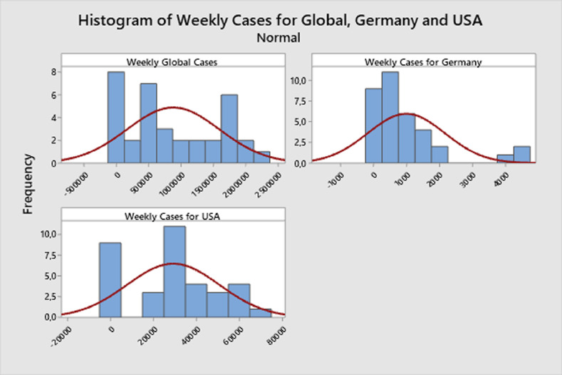
Germany has positive kurtosis, global and USA have negative kurtosis. As shown in Fig. 1 , the data distribution for Germany with large kurtosis displays tail data that exceeds the tails of the normal distribution.

Fig. 1.

Histogram of weekly cases for global, Germany and USA

In addition, distribution analysis was made for weekly case data. The results of goodness of fit test for weekly global cases are given in Table 2 . Fitting of the data to Lognormal, Normal, Exponential, 2-Parameter Exponential, Weibull, 3-Parameter Weibull, Largest Extreme Value, Smallest Extreme Value, Logistic and Gamma distributions was investigated.

Table 2.

Goodness of fit test for weekly global cases

Distribution	AD	P
Normal	1,259	<0,005
Lognormal	2,860	<0,005
Exponential	2,594	<0,003
2-Parameter Exponential	1,665	0,012
Weibull	2,039	<0,010
3-Parameter Weibull	1,667	<0,005
Smallest Extreme Value	1,564	<0,010
Largest Extreme Value	1,153	<0,010
Gamma	1,798	<0,005
Logistic	1,232	<0,005

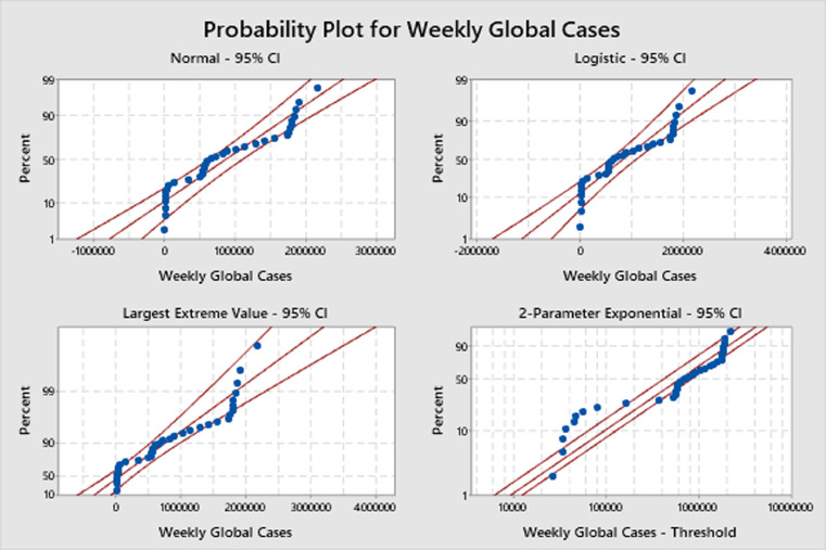
In Table 2, AD value represents Anderson-Darling test value. It is a measure of the deviations between the fitted line of the distribution and data points. The p-value is the probability showing that the data follow the distribution. In order to choose the best distribution, it is expected that the AD value is low and the p-value is high. The probability plot of the first four distributions with the lowest AD value is given in Fig. 2 . As seen in Fig. 2, Largest Extreme Value is the distribution that fits best for global weekly data.

Fig. 2.

Probability plot for weekly global cases

Estimated parameters of distributions for global weekly data are given in Table 3 . Using these parameters, proper similar data can be derived for distributions or used for estimation.

Table 3.

Estimates of distribution parameters for weekly global cases

Distribution	Location	Shape	Scale	Threshold
Normal	881.504	-	714.238	-
Lognormal	12,80563	-	1,93553	-
Exponential	-	-	881.504	-
2-Parameter Exponential	-	-	905.445	-23.941,9
Weibull	-	0,83125	820.779	-
3-Parameter Weibull	-	1,01121	910.043	-24.993
Smallest Extreme Value	1.241.170	-	668.737	-
Largest Extreme Value	542.319	-	580.244	-
Gamma	-	0,68580	1.285.360	-
Logistic	844.683	-	430.713	-

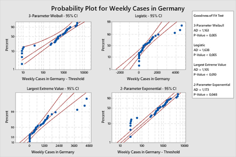
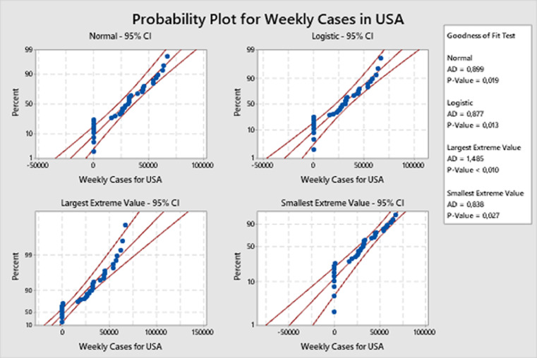
Similarly, the goodness of fit test was performed for the weekly case data of Germany and USA, and probability plots are given in Figs. 3 and 4 . Accordingly, the best fit distribution for Germany was found as largest extreme value and it was found as smallest extreme value for USA. The smallest extreme value distribution is skewed to the left and the largest extreme value distribution is skewed to the right. This skewness can also be seen in Fig. 1 for Germany, USA and global data.

Fig. 3.

Probability plot for weekly cases in Germany

Fig. 4.

Probability plot for weekly cases in USA

4. Short-term cumulative case forecasting

In this study, data of COVID-19 between 20/01/2020 and 18/09/2020 for USA, Germany and the global was obtained from World Health Organization website [16]. Furthermore, time series prediction model using machine learning methods is proposed to obtain the disease curve and forecast the epidemic trend. Linear regression, multi-layer perceptron, random forest and support vector machines methods were used for forecasting. The evaluation metrics described in the subsection below are used to compare these methods.

4.1. Evaluation metrics

In order to compare the estimation methods used in this study, root mean square error (RMSE), mean absolute percentage error (MAPE) and absolute percentage error (APE) metrics were used. By measuring APE, the consistency between the original value and the predicted value is calculated. These values are expected to be low when comparing. The following equations will express the APE, MAPE, and RMSE calculations:

$$APE(\%)=\left|\frac{y\left(i\right)-\widehat{y}\left(i\right)}{y\left(i\right)}\right|\times 100$$ (3)

$$MAPE(\%)=\sum _{i=2}^n\left|\frac{y\left(i\right)-\widehat{y}\left(i\right)}{y\left(i\right)}\right|\times \frac{100}{n-1}$$ (4)

$$RMSE=\sqrt{\frac{{\sum }_{i=2}^n{(y\left(i\right)-\widehat{y}\left(i\right))}^2}{n-1}}$$ (5)

where n shows observation number, y_i is the i-th observed value and ŷ_i is the i-th estimated value.

4.2. Results and discussion

Machine learning time series takes into account the time parameter and evaluates other inputs based on time. In this study, time feature is divided into sub-components as time index, weekly cases, 17 lagged variables of weekly cases, square of the time index, cube of time index and products of 17 lagged variables with time index. Thus, 38 different variables were extracted.

Dataset consist of weekly cumulative confirmed cases for 35 weeks. In machine learning methods, the data for the time series is divided into two groups as training and test data. In this study, 18 weeks were used for training and 17 weeks as test data.

After training and testing, APE, MAPE, RMSE values were found and are given in Table 4 for linear regression, multi-layer perceptron, random forest and SVM machine learning methods. In Table 4, it is seen that SVM method provides the best performance for the global, Germany and USA data. It is the method with the lowest value for RMSE, MAPE, and APE values. It is obviously seen that SVM achieved the best trend for all data.

Table 4.

Comparison of the methods.

Methods	Metric	Global	Germany	USA
Random Forest	MAE	269.274,0518	955,1736	42.496,719
	MAPE	2,0726	0,4477	1,5608
	RMSE	340.926,4251	1.387,0147	53.864,6539
Linear Regression	MAE	17.081,1363	224,0337	11.745,2812
	MAPE	0,1853	0,1125	0,3331
	RMSE	21.816,6988	324,0253	16.508,4263
MLP	MAE	139.330,4846	752,3291	19.819,1675
	MAPE	0,8179	0,381	0,6497
	RMSE	223.638,9972	832.688,26	26.713,8094
SVM	MAE	19.771,7317	191,0731	5.852,0147
	MAPE	0,1247	0,0918	0,1406
	RMSE	25.825,8366	329,196	9.531,6776

When Table 4 is examined in detail, SVM and linear regression methods have very close MAPE and RMSE values. Next comes the MLP method. The method with the worst performance is Random Forest. The Random Forest method has also failed in predicting the future.

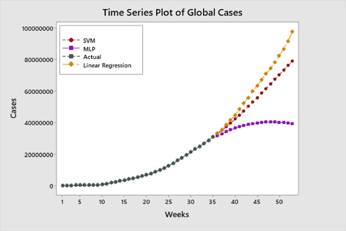
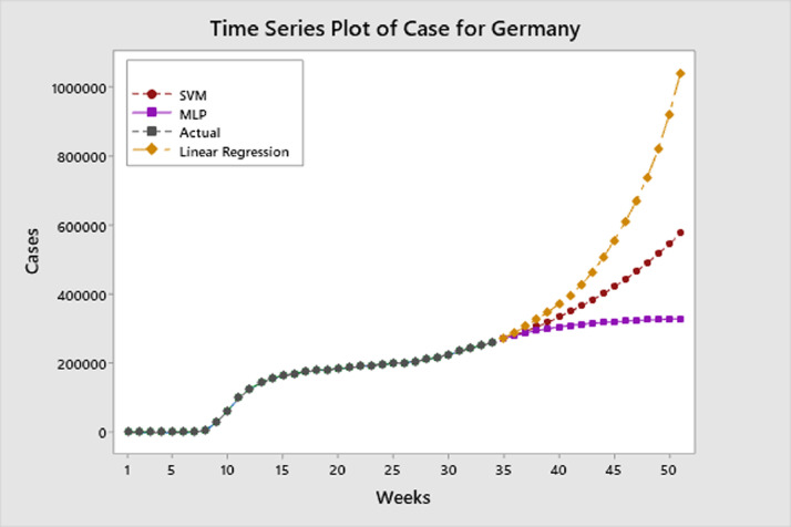
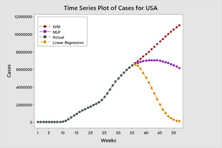
Accordingly, estimations were made with best three method for the global, Germany and USA for 17 weeks after 18/09/2020. These estimates are shown in Fig. 5, Fig. 6, Fig. 7 .

Fig. 5.

Prediction of weekly cumulative global cases

Fig. 6.

Prediction of weekly cumulative cases for Germany

Fig. 7.

Prediction of weekly cumulative cases for USA

Fig. 5 shows the future trend for global cumulative data. According to forecasts in Fig. 5, the global pandemic will peak at the end of January 2021 and an estimated approximately 80 million people will be cumulatively infected by using SVM method. Approximately 98 million people will be infected according to the linear regression method. For the MLP method, approximately 39 million people will be infected. The prediction of SVM, which is the best method according to performance metrics, seems more robust and realistic.

Fig. 6 shows the future trend for cumulative case data for Germany. According to forecasts in Fig. 6, Germany will peak at the end of January 2021 and an estimated approximately 580.000 people will be cumulatively infected by using SVM method. Approximately 1 million people will be infected according to the linear regression method. For the MLP method, 330.000 people will be infected. Performance metrics show that the estimation of SVM is more accurate.

According to forecasts in Fig. 7, USA will peak at the end of January 2021 and an estimated approximately 11 million people will be cumulatively infected by using SVM method. According to linear regression method, it enters a downward trend and approaches zero. This is not a realistic estimation. According to the MLP method, 6 million people will be infected. Once again, the prediction of SVM seems more realistic.

5. Conclusion

In this study, data of COVID-19 between 20/01/2020 and 18/09/2020 for USA, Germany and the global was analyzed. The distribution of the data is found as largest extreme value for global and Germany and smallest extreme value for USA. Then time series prediction model is proposed to obtain the disease curve and forecast the epidemic trend using machine learning methods. Linear regression, multi-layer perceptron, random forest and SVM machine learning methods were used for this purpose. The performances of the methods were compared according to the RMSE, APE, MAPE criteria. The results showed that the SVM method outperformed linear regression, multi-layer perceptron, random forest methods in modeling the Covid-19 data, and could be successfully used to diagnose the behavior of cumulative Covid-19 data over time. With the practical application of such machine learning time series methods, further research is expected to provide the most appropriate method for healthcare professionals to control and prevent future epidemics.

CRediT authorship contribution statement

Serkan Ballı: Investigation, Conceptualization, Methodology, Formal analysis, Validation, Writing - review & editing.

Declaration of Competing Interest

The author declares that he has no known competing financial interests or personal relationships that could have appeared to influence the work reported in this paper.

References

- 1.Ahmed N.K., Atiya A.F., Gayar N.E., El-Shishiny H. An empirical comparison of machine learning models for time series forecasting. Econom Rev. 2010;29(5–6):594–621. [Google Scholar]
- 2.Breiman L. Random forests. Mach Learn. 2001;45(1):5–32. [Google Scholar]
- 3.Brokamp C., Jandarov R., Rao M.B., LeMasters G., Ryan P. Exposure assessment models for elemental components of particulate matter in an urban environment: a comparison of regression and random forest approaches. Atmos Environ. 2017;151:1–11. doi: 10.1016/j.atmosenv.2016.11.066. [DOI] [PMC free article] [PubMed] [Google Scholar]
- 4.Das R.C. Forecasting incidences of covid-19 using box-jenkins method for the period july 12-septembert 11, 2020: a study on highly affected countries. Chaos, Solitons and Fractals. 2020;140:110248. doi: 10.1016/j.chaos.2020.110248. [DOI] [PMC free article] [PubMed] [Google Scholar]
- 5.Elfahham Y. Estimation and prediction of construction cost index using neural networks, time series, and regression. Alex Eng J. 2019;58(2):499–506. [Google Scholar]
- 6.Fanelli D., Piazza F. Analysis and forecast of covid-19 spreading in china, italy and france. Chaos, Solitons and Fractals. 2020;134:109761. doi: 10.1016/j.chaos.2020.109761. [DOI] [PMC free article] [PubMed] [Google Scholar]
- 7.Feroze N. Forecasting the patterns of covid-19 and causal impacts of lockdown in top ten affected countries using bayesian structural time series models. Chaos, Solitons and Fractals. 2020;140:110196. doi: 10.1016/j.chaos.2020.110196. [DOI] [PMC free article] [PubMed] [Google Scholar]
- 8.Guan W.J., Ni Z.Y., Hu Y., Liang W., Ou C., He J. Clinical characteristics of coronavirus disease 2019 in china. N top N Engl J Med. 2020;382(18):1708–1720. doi: 10.1056/NEJMoa2002032. [DOI] [PMC free article] [PubMed] [Google Scholar]
- 9.Kaxiras E., Neofotistos G., Angelaki E. The first 100 days: modeling the evolution of the covid-19 pandemic. Chaos, Solitons and Fractals. 2020;138:110114. doi: 10.1016/j.chaos.2020.110114. [DOI] [PMC free article] [PubMed] [Google Scholar]
- 10.Ribeiro M.H.D.M., Coelho D.S.L. Ensemble approach based on bagging, boosting and stacking for short-term prediction in agribusiness time series. Appl Soft Comput. 2020;86:105837. [Google Scholar]
- 11.Rosenblatt F. Principles of neurodynamics. perceptrons and the theory of brain mechanisms. Report No. VG-1196-G-8. Cornell Aeronautical Lab Inc, Buffalo NY, https://apps.dtic.mil/dtic/tr/fulltext/u2/256582.pdf. [Accessed: September 18, 2020]; 1961.
- 12.Sahin U., Sahin T. Forecasting the cumulative number of confirmed cases of covid-19 in Italy, UK and USA using fractional nonlinear grey bernoulli model. Chaos Solitons Fractals. 2020;138:109948. doi: 10.1016/j.chaos.2020.109948. [DOI] [PMC free article] [PubMed] [Google Scholar]
- 13.Shastri S., Singh K., Kumar S., Kour P., Mansotra V. Time series forecasting of covid-19 using deep learning models: India-USA comparative case study. Chaos, Solitons and Fractals. 2020;140:110227. doi: 10.1016/j.chaos.2020.110227. [DOI] [PMC free article] [PubMed] [Google Scholar]
- 14.Shirmohammadi-Khorram N., Tapak L., Hamidi O., Maryanaji Z. A comparison of three data mining time series models in prediction of monthly brucellosis surveillance data. Zoonoses Public Health. 2019;66(7):759–772. doi: 10.1111/zph.12622. [DOI] [PubMed] [Google Scholar]
- 15.Wang P., Zheng X., Li J., Zhu B. Prediction of epidemic trends in covid-19 with logistic model and machine learning technics. Chaos, Solitons and Fractals. 2020;139:110058. doi: 10.1016/j.chaos.2020.110058. [DOI] [PMC free article] [PubMed] [Google Scholar]
- 16.WHO. World health organization covid cumulative dataset. https://covid19.who.int [Accessed: September 18, 2020]; 2020.
- 17.Wieczorek M., Siłka J., Woźniak M. Neural network powered covid-19 spread forecasting model. Chaos, Solitons and Fractals. 2020;140:110203. doi: 10.1016/j.chaos.2020.110203. [DOI] [PMC free article] [PubMed] [Google Scholar]
- 18.Yadav M., Perumal M., Srinivas M. Analysis on novel coronavirus (covid-19) using machine learning methods. Chaos, Solitons and Fractals. 2020;139:110050. doi: 10.1016/j.chaos.2020.110050. [DOI] [PMC free article] [PubMed] [Google Scholar]
- 19.Yang J.H., Cheng C.H., Chan C.P. A time-series water level forecasting model based on imputation and variable selection method. Comput Intell Neurosci. 2017;2017:8734214. doi: 10.1155/2017/8734214. [DOI] [PMC free article] [PubMed] [Google Scholar]
- 20.Yesilkanat C.M. Spatio-temporal estimation of the daily cases of covid-19 in worldwide using random forest machine learning algorithm. Chaos, Solitons and Fractals. 2020;140:110210. doi: 10.1016/j.chaos.2020.110210. [DOI] [PMC free article] [PubMed] [Google Scholar]