Resolving the 3D landscape of transcription-linked mammalian chromatin folding

Tsung-Han S Hsieh; Claudia Cattoglio; Elena Slobodyanyuk; Anders S Hansen; Oliver J Rando; Robert Tjian; Xavier Darzacq

doi:10.1016/j.molcel.2020.03.002

. Author manuscript; available in PMC: 2021 May 7.

Published in final edited form as: Mol Cell. 2020 Mar 25;78(3):539–553.e8. doi: 10.1016/j.molcel.2020.03.002

Resolving the 3D landscape of transcription-linked mammalian chromatin folding

Tsung-Han S Hsieh ^1,^2,^3,^4,⁵, Claudia Cattoglio ^1,^2,^3,⁵, Elena Slobodyanyuk ^1,^2,^3,⁵, Anders S Hansen ^1,^2,^3,^5,⁶, Oliver J Rando ⁷, Robert Tjian ^1,^2,^3,^5,^*, Xavier Darzacq ^1,^2,^3,^4,^8,^*

PMCID: PMC7703524 NIHMSID: NIHMS1642102 PMID: 32213323

SUMMARY

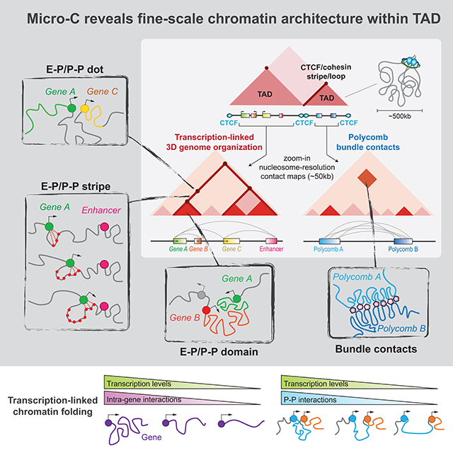
Whereas folding of genomes at the large scale of epigenomic compartments and topologically associating domains is now relatively well understood, how chromatin is folded at finer scales remains largely unexplored in mammals. Here, we overcome some limitations of conventional 3C-based methods by using high-resolution Micro-C to probe links between 3D genome organization and transcriptional regulation in mouse stem cells. Combinatorial binding of transcription factors, cofactors, and chromatin modifiers spatially segregates TAD regions into various finer-scale structures with distinct regulatory features including stripes, dots, and domains linking promoters-to-promoters (P-P) or enhancers-to-promoters (E-P), and bundle contacts between Polycomb regions. E-P stripes extending from the edge of domains predominantly link co-expressed loci, often in the absence of CTCF and cohesin occupancy. Acute inhibition of transcription disrupts these gene-related folding features without altering higher-order chromatin structures. Our study uncovers previously obscured finer-scale genome organization, establishing functional links between chromatin folding and gene regulation.

Keywords: Micro-C, enhancer-promoter (E-P) interactions, 3D genome, TAD, transcription, Pol II, CTCF, loop extrusion, 30-nm chromatin fiber

In Brief

Hsieh et al. describe chromatin folding at single-nucleosome resolution in mammalian cells using Micro-C, an enhanced chromosome conformation capture method. Micro-C uncovers genome-wide, fine-scale chromatin organizational features shaped by gene activity, transcriptional regulation, and gene silencing.

Graphical Abstract

graphic file with name nihms-1642102-f0001.jpg

INTRODUCTION

Chromatin packages the eukaryotic genome via a hierarchical series of folding steps ranging from individual nucleosomes to entire chromosome territories (Gibcus and Dekker, 2013). Structural analysis of chromosome folding has been revolutionized by the Chromosome Conformation Capture (3C) family of techniques, which uses proximity ligation of cross-linked genomic loci in vivo to estimate contact frequencies (Dekker et al., 2013). Interphase chromosome structures such as compartments (Lieberman-Aiden et al., 2009), topologically-associating domains (TADs) (Dixon et al., 2012; Nora et al., 2012), and CTCF and cohesin chromatin loops (Rao et al., 2014) have been characterized using 3C-based methods. Chromosome compartments correspond to large-scale active and inactive chromatin segments and appear as a plaid-like pattern in Hi-C contact maps at the megabase scale (Lieberman-Aiden et al., 2009). At the intermediate scale of tens to hundreds of kilobases, topologically associating domains (TADs) spatially organize the mammalian genome into continuous self-interacting domains. TADs are defined as local domains within which genomic loci come into contact with each other more frequently than with loci outside, and appear as square boxes along the diagonal of 3D contact maps (Dixon et al., 2012; Nora et al., 2012). Mounting evidence suggests that CTCF and cohesin mediate TAD formation via a loop extrusion mechanism (Fudenberg et al., 2016; Sanborn et al., 2015), wherein the cohesin ring complex entraps chromatin loci and extrudes chromatin until blocked by CTCF or other proteins. Stabilization of cohesin at CTCF sites gives rise to sharp corner peaks in contact maps, which are also referred to as loops or loop domains. Various studies have reported that TADs and loops influence transcriptional regulation (Bonev and Cavalli, 2016), and disruption of these structures can lead to certain diseases (Lupiáñez et al., 2015). Although CTCF and cohesin are thought to be required for essentially all aspects of genome folding below the level of compartments (Fudenberg et al., 2018), it remains unclear how the TAD-dominated organization contributes to transcriptional regulation, as acute disruption of TADs and loops only results in relatively modest effects on gene expression (Nora et al., 2017; Rao et al., 2017; Schwarzer et al., 2017; Sofueva et al., 2013).

Beyond CTCF- and cohesin-mediated structures, a classical model of transcription posits that cis-regulatory elements control gene expression via long-range enhancer-promoter interactions (also called E-P links) (Taatjes et al., 2004). Various models such as chromatin tracking, linking, or looping have been proposed to describe the mechanisms by which enhancers engage their cognate genes across long DNA distances (Furlong and Levine, 2018; Robson et al., 2019). Recent findings further suggest that local protein condensates may facilitate the spatial engagement of E-P links via homotypic attraction between condensates that have a similar chemical property (Furlong and Levine, 2018; Robson et al., 2019). Factors such as the general transcription machinery, co-activators (Mediator, YY1) (Beagan et al., 2017; Phillips-Cremins et al., 2013; Weintraub et al., 2017), and chromatin remodelers (Brg1) (Barisic et al., 2019) have been reported to mediate E-P links that direct transcriptional regulation. However, largely due to technical limitations of current techniques, structural details about how these fine-scale structures are organized in the genome, and whether transcription can drive the folding of 3D structures, remain to be explored by higher-resolution approaches. For example, the role of RNA polymerase II (Pol II)-mediated transcription in TAD formation and 3D genome organization in general remains controversial, with reports of disparate responses to transcription inhibition (Hug et al., 2017; Li et al., 2015; Rowley et al., 2017). Also, debates regarding the functional role of 3D structures in regulating Sonic hedgehog (shh) expression during embryonic development remain unsettled (Paliou et al., 2019; Symmons et al., 2016; Williamson et al., 2019). Hence, in addition to the emerging works that identified functional enhancers of interest (Arnold et al., 2013; Barakat et al., 2018; Korkmaz et al., 2016), a more comprehensive and higher-resolution method to reveal the fine-scale enhancer connectome is becoming increasingly crucial for studies of the 3D genome and gene regulation.

The resolution gap between 1D and 3D genomic maps as well as a paucity of known chromatin features below the level of TADs has significantly limited our understanding of gene regulation and its potential link to chromatin architecture. Such gene-specific structures and local nucleosome folding remain largely unexplored by genome-wide approaches in mammals. The existence of gene loops (O’Sullivan et al., 2004), or organization of beads-on-a-string into 30-nm chromatin fibers (Luger et al., 2012), and their functional relevance to transcription regulation, all remain hotly debated. Here, we employed Micro-C, an assay that overcomes the resolution limitations of Hi-C by measuring contacts between pairs of crosslinked nucleosomes, to investigate chromatin organization in mouse embryonic stem cells at a resolution of ~200 bp (Hansen et al., 2019; Hsieh et al., 2015, 2016). We focused on dissecting the principles of chromatin folding below the scale of TADs in order to probe how transcription and transcription regulators may contribute to this more refined scale of 3D genome architecture in the complex milieu of mammalian chromosomes.

RESULTS

Micro-C reveals fine-scale chromatin organizational features in mammalian cells

To effectively interrogate features below the level of TADs that are largely inaccessible by conventional Hi-C analysis, we employed the Micro-C protocol for mapping chromosome folding at single nucleosome resolution (~100–200 bp) in mammalian cells (Figure 1A and S1–AB). We generated 38 biological replicates from mouse embryonic stem cells (mESCs) and pooled the replicates after confirming high reproducibility (>0.95) across samples (Figure S1C). In a side-by-side comparison of pooled Micro-C (2.64B reads) to the current highest-depth Hi-C data (3.33B reads) (Table S1) (Bonev et al., 2017), Micro-C recapitulated all the reported chromatin structures such as compartments, TADs, and loops (Figure S1D), with high reproducibility scores and comparable data quality (Figure S1E–F). Notably, in addition to the scale over 20 kb at which Micro-C and Hi-C generated nearly identical data (reproducibility >0.9), Micro-C can also assess local chromatin folding at the scale of 100 bp to 20 kb, as shown by a genome-wide averaged contact frequency analysis (Figure 1B). This length range covers fine-scale chromatin structures such as genes (median=~28 kb) and promoter-promoter (P-P) or enhancer-promoter (E-P) interactions (~5–200 kb measured by HiChIP) (Di Giammartino et al., 2019; Mumbach et al., 2017), and reveals significantly more loop-like structures than Hi-C analysis at similar sequencing depth (n=29,548 by Micro-C vs. n=6,006 by Hi-C; loops appear as “dots” or “peaks” in the contact maps) (Figure 1C and Table S2). Specifically, Micro-C robustly detects single E-P or P-P linkages with a sharp and robust signal, while standard Hi-C detects weak enrichment, if any, in most of these cases (Figure S1D). Consequently, our results demonstrate that, at coarse resolution, Micro-C yields a qualitatively and quantitatively similar measurement of 3D genome organization compared to Hi-C analysis. Crucially, Micro-C overcomes the current resolution gap of Hi-C at the fine scale, which now allows us to investigate more detailed chromatin structures that may be functionally relevant to gene regulation.

Figure 1. — (A) Overview of Micro-C method for mammals. (B) Comparison of interaction decaying rates of Micro-C and Hi-C. X-axis: the distance between contact loci from 100-bp to 10-Mb. Y-axis: contact density normalized by sequencing depth. (C) Comparison of identified loop numbers in Micro-C and Hi-C. (D-E) Snapshots of 65 kb of Micro-C and Hi-C contact maps at single nucleosome resolution. Each dot on the contact matrix represents the contact intensity between a pair of nucleosomes. Contact maps were annotated with gene boxes and aligned with multiple 1D chromatin tracks. Standard heatmap shows the gradient of contact intensity for a given pair of bins. The color scheme is used for Micro-C maps throughout the manuscript. Features like E-P domains, stripes, and dots enriched at stripe intersections are highlighted. Black arrows indicate CTCF-negative stripes. Micro-C analyses in wild-type mESC were generated from pooled 38 biological replicates throughout the manuscript.

Identification of E-P stripes, dots, and domains

Taking advantage of the enhanced Micro-C resolution, we next searched for principles underlying short-range chromatin folding by integrating our Micro-C contact maps with 48 public genomic datasets (detailed description in Table S3). Visual inspection of a local 65-kb nucleosome-resolution map identified several finer self-interacting domains spanning ~5–10 kb along the genome (Figure 1D), encompassing either single genes (e.g., Eif2b4), multiple genes (e.g., Snx17 and Zfp513), or intergenic regions (e.g., between the divergent genes Nrbp1 and Ppm1g).

Stripes or flames correspond to lines extending from the diagonal in contact maps and are thought to result from the process of cohesin-mediated loop extrusion (Fudenberg et al., 2018; Vian et al., 2018). In Hi-C, stripes are visible at the level of hundreds of kb. But here, we uncovered a series of much smaller (~10–50 kb) and nested stripes extending from the border of local self-interacting domains. These stripes predominantly link promoter-promoter or promoter-enhancer sites (Figure 1D, P-P or E-P stripes), and often form sharper “loop-like” structures at their intersections (Figure 1D, P-P or E-P dots). Indeed, the stripes colocalize with transcription start sites (TSSs) and some intergenic regions, and appear to be enriched with active transcription features such as Pol II binding sites, accessible chromatin regions, and active histone marks, and do not predominantly correspond to CTCF or cohesin binding (Figure 1D–E). Thus, these CTCF and cohesin-negative stripes and dots do not appear to simply represent features of the loop-extrusion process, and could be mediated by other proteins and mechanisms (Di Giammartino et al., 2019; Mumbach et al., 2017; Zheng et al., 2019). Since E-P or P-P communication is typically associated with one or multiple local self-interacting domains, including stripes extending from domain borders and focal signals at their intersection, we hereafter simply call these features E-P domains, stripes, and dots. We confirmed the presence of E-P stripes and domains in mESCs at several other genomic regions containing functionally validated enhancers that had gone undetected by Hi-C analysis (Figure 1D and S1G–H) (Bonev et al., 2017). Notably, there were no discernible differences in stripes or dot structures between enhancers and “super-enhancers” at these loci (Figure S1G–I) (Lizio et al., 2015; Moorthy et al., 2017; Whyte et al., 2013). In summary, nucleosome-resolution Micro-C contact maps bring into sharp focus previously obscured chromatin structures within TADs that include E-P stripes, dots, and domains, and these finer-scale structures appear to form in a gene-dependent manner.

Genome-wide characterization of E-P stripes and domain boundaries

We next tested whether genome-wide insulation score analysis (Crane et al., 2015) could characterize the boundaries of nested E-P stripes and domains in an unbiased way. A comprehensive insulation analysis using 200-bp to 20-kb resolution Micro-C data revealed boundaries at various scales in compartment A, while compartment B did not show any apparent fine-scale chromatin folding (Figure S2A–C and Table S4). These results suggest that very distinct chromatin folding mechanisms may be at play between compartment A versus B, likely related to active transcription. To focus on finer-scale transcription-associated chromatin folding, we will mainly discuss the analysis of chromatin features in the active compartment (unless otherwise mentioned) and include some key compartment B analyses in the supplement.

Consistent with previous reports by Hi-C (Gibcus et al., 2018), ~4,500 TAD structures were detected by using 20-kb resolution boundary metrics (Figure S2A–B). Using 200-bp to 1-kb resolution metrics, we identified ~136,223 fine-scale boundaries in the active compartment that had previously gone undetected (Dixon et al., 2012) (Figure 2A–C and S2A–B), and whose insulation scores precisely peak at the borders of E-P stripes and domains (Figure 2A and S2D). The much higher abundance of fine boundaries led us to ask: what genetic and chromatin features are enriched at these boundaries? We found that these boundaries have a clear relationship with gene structure, typically encompassing one to two genes, and have a flanking length ranging from 5 to 40 kb (Figure 2D). Boundaries in the active compartments predominantly localize to CpG islands, promoters, and tRNA genes (Figure 2E), and tend to be closer to the TSS (Figure S2E), while boundaries in the inactive compartment are found in chromosomal regions rich in repeats (Figure S2F). In summary, high-resolution insulation metrics precisely locate the borders of E-P stripes and domains, and these structures are proximal to promoters and cis-regulatory elements in active compartments.

Figure 2. — (A) Example of Micro-C boundary identification. Nucleosome-resolution contact maps were plotted for an 85-kb region on chr6. The browser tracks show insulation scores and called boundaries by the data resolution from 200 bp to 20 kb. Called boundaries are indicated as black lines. (B) Validation of the called boundaries by pile-up analysis. Boundaries within compartment A were centered at a matrix that is 100x larger than the bin size. The contact map was normalized by matrix balancing and distance, with positive enrichment in red and negative signal in blue, shown as the diverging colormap with the gradient of normalized contact enrichment in log2. The color scheme and the normalization method are used for normalized matrix throughout the manuscript unless otherwise mentioned. (C) Heatmap and histogram profile of insulation scores at 200-bp, 1-kb, and 20-kb resolutions. Each row represents insulation scores across a 100x larger region with the called boundary at the center. Histogram at the bottom of the plot shows the genome-wide average of the insulation score. (D) Length distribution of boundary intervals within compartment A. The median size of the boundary interval is annotated below each box. (E) Genomic features of boundaries within compartment A. Bar graph shows the log2 enrichment of genomic features at boundaries identified by 200-bp resolution.

Biochemical predictors of fine-scale boundary position and strength

The observation that fine-scale boundaries tend to overlap with promoters and cis-regulatory elements suggests a potential connection between chromatin folding and gene regulation. To further investigate this correlation, we first compared boundary locations with nucleosome occupancy (Carone et al., 2014; Ishii et al., 2015) (Figure 3A and S3A, Table S3). Overall, the boundaries are enriched for transcription factor binding sites and dynamic nucleosomes (also known as “fragile nucleosomes”), since signals from short fragments (1–100 bp) corresponding to transcription factor binding are substantially higher at these boundaries. Boundary strength is also correlated with nucleosome occupancy (Figure S3B), as stronger boundaries exhibit a higher level of nucleosome depletion and often center at nucleosome-depleted regions (NDRs).

Given that the majority of boundaries are flanked by +1 and −1 nucleosomes immediately upstream and downstream of a gene’s TSS (Figure 3A and S3A), we next asked how local histone modifications and protein binding profiles might relate to boundary properties. To systemically identify factors most predictive of fine-scale boundary location or strength, we applied a generalized linear regression model based on genome-wide chromatin data (Figure S3C–D). Key predictors (28 out of 48) were obtained after removing redundant factors using lasso regularization. The regression coefficients revealed that transcription factors, architectural proteins, and repressive regulators are the most predictive factors of boundary properties to varying degrees (Figure 3B). Consistent with the finding that E-P structures are enriched at the boundaries, CTCF or cohesin, chromatin accessibility, Mediator, active histone marks, and transcription factors are all positive predictors of boundary location, while H3K27me3, H3K9me2 and CBX proteins are negative predictors of boundary location (Figure 3C). Strikingly, CTCF or cohesin are the best predictors of boundary location but only moderate predictors of boundary strength. Instead, chromatin accessibility and transcriptionally active chromatin most strongly predict boundary strength (Figure 3D).

To further explore the relationship between chromatin features and boundary strength, we quantified the boundary strength over 11 chromatin states defined by ChromHMM (Ernst and Kellis, 2012), confirming that boundaries enriched at active promoters and enhancers have the strongest insulation activity (Figure 3E and S3E–F). Signal intensities of several candidates around the boundary regions also coincide with the strongest boundary (Figure S3G). Thus, unlike large-scale chromatin structures (e.g., TADs and loops) which appear to be demarcated mainly by CTCF and cohesin (Rao et al., 2014), the fine-scale chromatin folding shows a wide spectrum of boundary markers.

A combination of chromatin features discriminates subgroups of boundaries

We next sought to examine whether combinatorial chromatin patterns can segregate the finer-scale boundaries into subgroups. To dissect the properties of a boundary, we plotted single boundaries in 2D t-Distributed Stochastic Neighbor Embedding (t-SNE) space according to their protein-binding profile (Figure S3H–I). Consistent with the boundary enrichment in the ChromHMM states (Figure S3E–F), we can classify the boundaries into at least five partially overlapping subgroups based on their biochemical and functional features (Figure 3F). We denote the five boundary subgroups as follows (see Table S5 for details): 1) transcription-dependent (~14%); 2) enhancer-related I, ES cell-specific (~9%); 3) enhancer-related II, constitutive (~15%); 4) repressive (~3%); and 5) CTCF and cohesin-mediated (~15%). Notably, chemical modifications on boundary-flanking nucleosomes not only recapitulate the major subgroups (Figure 3G) but also identify some rare populations. For instance, H3K79me2-enriched boundaries might be related to transcription, DNA replication, and repair (Nguyen and Zhang, 2011).

In more detail, transcription-dependent boundaries are strongly enriched for active features such as Pol II and transcription factors, consistent with our findings that active transcription demarcates TADs into finer-scale E-P structures. Enhancer-related boundaries occupy two distinct t-SNE spaces, one enriched with H3K4me1, Esrrb, and Nanog (Enhancer I), and another enriched with H3K27ac, Mediator, and Yy1 (Enhancer II). This distinction suggests that Enhancer I boundaries might be cell-type specific, while the Enhancer II group includes constitutive boundaries across cell types. Strikingly, although CTCF and cohesin appear to be strongly predictive of boundary location, their binding describes a subgroup of boundaries clearly separated from E-P boundaries in the t-SNE space (also in k-means clustering, data not shown). This implies that CTCF and cohesin boundaries might be architectural and confine chromatin topology through TADs. Finally, elevated H3K4me3 and H3K27me3 signals corresponding to the Polycomb complex highlight a subset of boundaries that demarcate bivalent chromatin. These bivalent boundaries may facilitate rapid activation of certain genes during mESC differentiation (Bernstein et al., 2006).

We conclude that Micro-C boundaries are heterogeneous and fall into distinct subclasses, suggesting that multiple distinct mechanisms might contribute to finer-scale chromatin folding. Specifically, active promoters and cis-regulatory elements are associated with the strongest boundaries (Figure 3E and S3J) that spatially segregate kb-sized regions into distinct E-P domains, and at least one subgroup of the domains appears to be cell type-specific. These CTCF- and cohesin-negative structures emerge as a crucial link between chromatin folding and transcription regulation.

Transcription factors mediate chromatin architecture within TADs

To understand how these fine-scale chromatin structures fold within TADs, we inspected Micro-C maps thoroughly in a 600-kb TAD (Figure S4A) and found that E-P stripes and domains interact with each other to form nested structures at scales of tens to hundreds of kilobases (Figure S4B–C). Overall, the stripes extending from domain boundaries connect promoters to promoters (P-P links) (Figure 4A and S4B–C, red arrows), enhancers to promoters (E-P links) (Figure 4B and S4B–C, green arrows), CTCF or cohesin loops (Figure S4B–C, purple arrows), and even TSSs to TTSs within the same gene (gene loops) (Figure 4A and S4B–C, pink arrows). Interestingly, previous studies reported that Polycomb repressive regions interact with each other through “loop” structures (Joshi et al., 2015; Schoenfelder et al., 2015; Vieux-Rochas et al., 2015). However, instead of forming focal contact enrichments, we found that most H3K27me3-rich regions form nested sets of chromatin contacts in Micro-C maps, as one patch of repressive chromatin hooks-and-loops to another patch (Figure 4C and S4D, blue arrows). Such bundle interactions are often delimited by a broad region of H3K9me2 (Figure 4C and S4D, gray arrow). Thus, whereas Polycomb interactions appear as blobs or loops in Hi-C, the higher resolution of Micro-C resolves the ultrastructure of these interactions as nested sets of chromatin contacts.

Genome-wide analysis of paired loci (Table S6) further confirmed ubiquitous dots linking E-P and P-P loci (Figure 4D) and genomic loci bound by various transcription and chromatin factors (Figure S5A–B), while Pol II-associated sites are mutually exclusive from repressive chromatin and Pol I and Pol III genes (Figure S5A–B). Importantly, the E-P and P-P dots are persistent at a similar level (only ~5–10% decrease) after computational removal of nearby CTCF and cohesin peaks (Figure 4E and S5A), suggesting that, in addition to CTCF, protein complexes that associate with promoters and enhancers can halt stripe extension and result in dot conformation along the stripe. In sum, cis-regulatory elements and their associated proteins appear to significantly contribute to dot formation with varying degrees of strength.

We next explored how different proteins shape local cis-interactions by 2D pile-up contact maps (Figure 4F–G). Consistent with previous studies (Hansen et al., 2019; Kraft et al., 2019; Vian et al., 2018), CTCF or cohesin binding sites colocalize with strong boundaries that prevent interactions up to Mb, and are associated with loop-extrusion stripes extending up to ~300 kb (Figure 4F–G and S5C). Unlike CTCF or cohesin, Pol II and active histone modifications mark robust short-range boundaries but are associated with weaker long-range insulators (Figure 4F–G and S5C). Evident fine-scale stripes extend beyond Pol II-occupied sites, likely a result of combining gene, E-P, and cohesin stripes. Interestingly, contact maps centered at enhancers (i.e., sites occupied by Mediator, pluripotency factors like Nanog, and cofactors like P300) show distinctive interactions connecting their upstream and downstream genomic loci at lengths between 10 and 100 kb (Figure 4F–G and S5C, black arrows). We speculate that a single enhancer may contact one to multiple genomic loci in spatial proximity.

Together, this analysis suggests that transcription factors and co-activators tend to associate with much finer or more proximal chromatin features (e.g., E-P stripes and dots), perhaps with multiple contact partners (Figure S5D), whereas CTCF and cohesin preferentially mediate long-range structures (e.g., TADs).

Pol II-dependent transcription drives gene folding

The direction of Pol II elongation (or gene orientation) is one of the major determinants of chromatin folding in yeast (Hsieh et al., 2016). In line with previous findings, we also found a correlation between gene orientation and the directionality of E-P or P-P stripes in mammals – E-P or P-P stripes usually extend toward the same direction as Pol II elongation (see examples in Figure 4A–B and S4B–C; genome-wide analysis in Figure S5E–F). This observation raises the question: could Pol II and active transcriptional processes be key drivers mediating these fine-scale chromatin structures?

We previously reported that gene-specific compaction levels are anti-correlated with transcription rate in the budding yeast Saccharomyces cerevisiae (Hsieh et al., 2015). This suggested that active transcription influences the unfolding of genes, but inactive transcription promotes gene compaction (Eagen et al., 2015). Does this principle also hold in mammals? We first plotted the density of Micro-C counts within each gene against its Pol II enrichment (Figure 5A). Surprisingly, in stark contrast to the findings in budding yeast, gene compaction levels are positively correlated with transcriptional activity (Spearman’s Rho=0.6). We corroborated this result by comparing gene folding levels by both unscaled (Figure 5B) and scaled (Figure S5E) pile-up analyses. Interactions are notably more pronounced within highly transcribed genes and genes with elevated levels of bound Pol II (Figure 5B and S5E–F) compared to lower-expressed genes. In addition to gene folding, P-P links also correlate with transcriptional activity (Figure 5C and controls in Figure S5G). The TSSs of highly transcribed genes often contact other TSSs with high transcription rates, while the TSSs of weakly transcribed genes show a decreased contact probability to other TSSs. Several P-P links are detectable even in the absence of CTCF and cohesin binding sites nearby (± 5 kb, Figure 5C). In contrast, transcription termination sites (TTSs) do not appear to contact other TTSs (Figure S5H) but show moderately higher preference for interaction with their own TSSs (Figure S5I, examples in Figure 4A and S4B), possibly forming gene crumples or loop structures (Hsieh et al., 2015; O’Sullivan et al., 2004; Tan-Wong et al., 2012). Together, these results suggest that the levels of gene folding and P-P links positively correlate with the transcriptional activity at these loci.

Figure 5. — (A) Scatter plot of gene compaction with transcriptional activity. X-axis: Pol II ChIP signal enrichment. Y-axis: contact density per gene square surface, bp². (B) Pile-up analysis of TSS-centered chromatin structure for short- (top) and long-range (bottom) structures. (C) TSS-mediated chromatin links. Genome-wide averaged contact maps are plotted by the paired TSSs that have been sorted by transcriptional activity into high, mid, and low. TSSs with CTCF or CTCF and SMC1A located within ±5 kb were excluded from this analysis.

To further dissect the functional relationship between gene structure and transcriptional activity we acutely inhibited transcription by treating cells for 45 minutes with either triptolide or flavopiridol, drugs that inhibit promoter melting and productive elongation, respectively (Figure 6A). Pol II ChIP-seq confirmed that transcription elongation was about 2- to 3-fold reduced after 45 minutes of drug treatments (Figure 6B and S6A–B). Acute inhibition of transcription had little effect on global chromatin organization at the scale of compartments, TADs, and loops (Figure 6C and S6C). Pol II inhibition also did not affect the strength of the fine-scale boundaries (Figure 6D and S6D). This result is consistent with the previous observation that DNA-binding transcription factors, CTCF, and cohesin may be sufficient to maintain the global chromatin configuration in mammalian cells, as Pol II inhibition also had a negligible effect on chromatin organization in the mouse and fly embryo (Du et al., 2017; Hug et al., 2017; Ke et al., 2017). However, the intensities of gene stripes significantly decreased upon Pol II inhibition (~1.25-fold decrease), and enhancer stripes became moderately reduced, while CTCF stripes remained largely unaltered (Figure 6E and S6E). Also, although Pol II inhibition did not significantly affect the E-P dot intensity, P-P and E-P stripes were greatly reduced (Figure 6F). Unaffected tRNA loci confirmed the drug specificity to Pol II mechanisms (Figure S6F). In sum, these findings suggest that Pol II drives chromatin folding such as P-P and E-P stripes at the gene level but has little or no effect on higher-order chromatin organization (Figure 6G and S6G). Transcription factors and co-activators engaging with promoters and enhancers may be sufficient to stabilize E-P or P-P links, since the structure is also less susceptible to Pol II inhibition (Figure 6G and S6G).

Figure 6. — (A) Schematics describing the mechanism of Pol II inhibition. (B) Pol II enrichment around TSS. Genome-wide Pol II ChIP-seq signals (2 biological replicates) are plotted across −1-kb to +10-kb regions from TSS for each condition. (C) Comparison of whole-genome contact density decaying curves. X-axis: the distance between contact loci from 100-bp to 10-Mb. Y-axis: contact density normalized to sequencing depth. (D) Comparison of genome-wide averaged insulation score. Micro-C data binned in 400-bp resolution were used in the insulation analysis here. Insulation intensities are plotted over a ±10kb region from the boundaries. (E) Comparison of promoter-, enhancer-, or CTCF-originating stripes after Pol II inhibition. Pile-up matrices were plotted at either 200-bp or 1-kb resolution as shown in the figure. (F) Comparison of P-P and E-P dots and stripes. Genome-wide averaged pile-up matrices are plotted by the paired loci. (G) Model of Pol II machinery driving E-P or P-P chromatin folding. Micro-C analyses in Pol II inhibition were generated from pooled 3 biological replicates.

Ligation orientation sheds light on CTCF loop topology and secondary chromatin folding

Micro-C captures contacts between any given nucleosome or TF-binding site (N) and its interacting partner (N+1, N+2, N+3, etc.) in all four scenarios of contact directionalities (Figure 7A and S7A). This allowed us to probe chromatin contact topology around CTCF-mediated loops and short-range nucleosome folding features such as 30 nm chromatin fibers in vivo.

Figure 7. — (A) Decaying curves of inter-nucleosomal contacts zoomed in to the distance between 200 bp and 5 kb. X-axis: the distance between contact loci. Y-axis: contact density normalized by sequencing depth. The orientations of read pairs facing toward one another are shown in different colors. Schematics illustrate the inter-nucleosomal contacts. Ligated nucleosomes are painted in pink. (B) Contact frequency between loop anchors with pairs of convergent CTCF motifs. Contacts in the orientations of 3’-to-5’ and 5’-to-3’ ligation are plotted separately and centered at the CTCF binding motif. Blue box: CTCF binding motif and its orientation. Green circle: extruding cohesin complex. Red dashed line: ligated DNA ends. C) Interaction decaying curves of mouse and yeast Micro-C data. Here we only showed the ligation products in 5’-to-3’ orientation. (D) Interaction abundance of N to N+X with distance. Curve indicates the slopes between the peak point of N+2 and N+X in Figure 7C. X-axis: the distances in units of nucleosomes. Y-axis: the slope of the indicated N to N+X. (E) The two-start zig-zag tetra-nucleosome stacks. The colored dots represent the ligated partners between N to N+X in the 5’-to-3’ orientation. (F) Models of fine-scale chromatin folding.

The current prevailing view is that CTCF-mediated chromatin loops are stabilized by DNA-extruding cohesin as it encounters a pair of convergent CTCF motifs (Fudenberg et al., 2016; Sanborn et al., 2015) (Figure 7B, cartoon model). To examine the putative loop extrusion model, we analyzed contact probabilities between the regions immediately upstream (5’-to-3’) and downstream (3’-to-5’) of loops anchored by convergent CTCF sites, and expected to find similar contact frequencies. Strikingly, the analysis revealed that 5’-to-3’ ligation events are the predominant contact orientation between the loop anchors, while the frequency of 3’-to-5’ ligations is ~2-fold less than expected (Figure 6B). This result highlights an asymmetric topology of CTCF-anchored loops, wherein the DNA ends on the loop extrusion side are not readily available for proximity ligation, possibly because the cohesin complex or other proteins physically block DNA ends or pull the two DNA templates away from each other.

We next explored potential second-order chromatin folding, popularly known as the 30-nm fiber. Dominant models for 30-nm fibers include the one-start solenoid helix model and the two-start zig-zag model, which differ in their periodicity, nucleosome spacing, and linker histone binding (Figure S7B) (Luger et al., 2012; Robinson and Rhodes, 2006). However, evidence for the existence of a 30-nm chromatin fiber in vivo has been elusive. A few studies have characterized local nucleosome folding by imaging or genomics approaches, finding some evidence of a tri- or tetra-nucleosome motif in yeast (Hsieh et al., 2015) and two-start helical fibers in human (Grigoryev et al., 2016; Risca et al., 2016). We thus interrogated Micro-C data to probe for evidence of 30-nm chromatin fibers in mammalian cells (Figure 7C–E and S7C–F). Interestingly, we observed a distinctive pattern of nucleosomal folding in mouse cells that supports the two-start zig-zag model (or zig-zag tetra-nucleosome folding) (Dorigo et al., 2004; Schalch et al., 2005). The abundance of ligation products for N to N+2 is nearly identical to N to N+3, and N to N+4 is also similar to N to N+5, and so forth up to ten nucleosomes away (Figure 7D and S7E, black arrows), consistent with prior cryo-EM results (Song et al., 2014). In contrast, the slopes in the yeast data appear to monotonically decrease without apparent periodic patterns (Figure 7C–D and S7C–E). Therefore, we conclude that an extended zig-zag path of chromatin folding can be detected in mES cells, which may consist of at least 2–3 tetra-nucleosome stacks (Figure 7E), while yeast secondary chromatin folds into a loose zig-zag-like structure that contains sparse tri- or tetra-nucleosome motifs.

DISCUSSION

How much the spatial architecture of mammalian genomes segregated into compartments, TADs, and loops actually impacts gene regulation remains hotly debated (Rowley and Corces, 2018; Steensel and Furlong, 2019). Recent findings suggest that genome topology and transcription are only loosely linked at the level of TADs and loops (Bonev et al., 2017; Hug et al., 2017; Li et al., 2015; Nora et al., 2017; Rao et al., 2017; Rowley et al., 2017; Sofueva et al., 2013), suggesting that there may be additional layers of structures that more directly relate to gene regulation. One of the key missing pieces to connect 3D genome architecture to transcription has been the inability of Hi-C to attain the resolution necessary to discern gene-level features of chromatin. Here, we employed Micro-C, which dissects chromosome folding in mammals at scales from single nucleosomes to the whole genome. Our high-resolution Micro-C contact maps have revealed several finer-scale features that justify an updated model for 3D genome organization at the resolution relevant to gene regulation (Figure 7F). In particular, we find that E-P and P-P links act as a hub to connect gene and cis-regulatory elements while also demarcating regions below the level of TADs into distinct chromatin domains.

Mechanisms of E-P and P-P interactions

Micro-C reveals that E-P and P-P interactions often manifest as stripes extending from the borders of fine-scale chromatin domains and that these stripes can link multiple genes or genes and enhancers together. We propose three mechanisms that could mediate the E-P and P-P communication. First, Pol II may drag “sticky” promoters and enhancers along with the transcriptional machinery during elongation until colliding with another large protein complex such as a transcription preinitiation complex or cohesin complex (Figure 6G, cartoon model). As the elongating complex is unable to pass through these structural blockades, we often observe “dots” at the ends or intersections of stripes (Figure 1D, 4A–B, S4B–C). Our finding that acute Pol II transcription inhibition disrupts both enhancer and promoter stripes is consistent with this model (Figure 6). Second, when the transcriptional machinery and cohesin complex collide, Pol II can assist the cohesin-associated loop extrusion machinery (Busslinger et al., 2017), which may also result in the formation of E-P or P-P stripes. The recent finding that CTCF or cohesion-mediated stripes associate with active enhancers and gene expression at the Epha4 developmental locus provides an example of this model with a functional readout (Kraft et al., 2019). However, yeast has similar transcriptional machineries and SMC complexes, but no stripe and loop structures were found during log phase, implying that active replication may act as a dominant force to disrupt these transcription-related structures in yeast (Hsieh et al., 2015, 2016). Third, multiple promoters and enhancers may be trapped within a regulatory protein and DNA hub (Figure S5D, cartoon model). These interactions are expected to be sufficiently stable and in close enough proximity to be captured by chemical crosslinking. Evidence from pile-up analyses of enhancer factors (Nanog, P300) as well as single loci with a stripe linking multiple enhancers supports this mechanism (Figure 4). Consistently, HiChIP analysis of Klf4 and H3K27ac revealed enhancer hubs that were correlated with cell-type specific gene regulation (Di Giammartino et al., 2019). We anticipate that these three models may not be mutually exclusive and could function together in vivo. Further functional studies by deleting enhancers or relevant factors will be informative to dissect the detailed mechanisms of E-P and P-P stripe formation.

How does Pol II mediate fine-scale gene folding?

Gene-specific and local nucleosome folding have been poorly explored by genome-wide approaches in mammals. Remarkably, although gene folding is dependent on transcriptional activity as seen in yeast (Hsieh et al., 2015), in mammals we found an inverse relationship. Unlike the yeast situation, in mammalian cells gene stripes and intra-gene interactions are highly enriched in actively transcribed genes. This may reflect a more complicated transcriptional regulatory mechanism in mammals. We envision two potential models to describe the transcription and Pol II-dependent gene folding. First, gene folding may be mediated by “sticky” Pol II as described above (Figure S6G, (i)). Alternatively, the promoter and related cis-regulatory elements could come together inside a Pol II hub, while Pol II and other factors deliver a range of chromatin elements into the hub for transcription (Figure S6G, (ii)). Acute Pol II inhibition only disrupts gene and enhancer stripes, but global chromatin folding does not change, indicating that preinitiation complex assembly and Pol II elongation might only account for a portion of chromatin folding, particularly at the scale of individual genes. Nevertheless, we cannot rule out the possibility that a short period of Pol II inhibition may not completely shut down transcriptional activity and evict preloaded Pol II that could continue elongating through a long gene. Furthermore, although acute depletion of CTCF and cohesin largely abolishes TADs, how they may affect E-P structures and gene-level folding remains to be determined. High-resolution Micro-C maps can be used to tackle these questions and provide additional links between fine-scale chromatin folding and gene regulation.

Here we have revealed a previously unknown layer of chromatin folding in mammals. We expect that further studies that combine nucleosome-resolution chromatin maps with live-cell single-molecule imaging or single-cell technologies will further refine our understanding of chromatin folding and its functions in mammalian gene regulation.

STAR METHODS

LEAD CONTACT AND MATERIALS AVAILABILITY

This study did not generate new unique reagents. Further information and requests for resources and reagents should be directed to and will be fulfilled by the Lead Contact, Xavier Darzacq (darzacq@berkeley.edu).

EXPERIMENTAL MODEL AND SUBJECT DETAILS

Cell culture

JM8.N4 mouse embryonic stem cells (Pettitt et al., 2009) (male mESCs; Research Resource Identifier: RRID:CVCL_J962; obtained from the KOMP Repository at UC Davis) were grown and handled as described at https://www.komp.org/pdf.php?cloneID=8669. Briefly, mES cells were grown on plates pre-coated with a 0.1% autoclaved gelatin solution (Sigma-Aldrich G9391) under feeder-free conditions in knock-out DMEM with 15% FBS and LIF (500 mL knockout DMEM (ThermoFisher #10829018), 6 mL MEM NEAA (ThermoFisher #11140050), 6 mL GlutaMax (ThermoFisher #35050061), 5 mL Penicillin-Streptomycin (ThermoFisher #15140122), 4.6 μL 2-mercaptoethanol (Sigma-Aldrich M3148), 90 mL fetal bovine serum (HyClone Logan, FBS SH30910.03 lot #AXJ47554)) and LIF. mES cells were fed with fresh medium daily and passaged every two days by trypsinization.

METHOD DETAILS

Overview of Micro-C experiment

Mammalian Micro-C protocol was modified from the original protocol for yeast in (Hsieh et al., 2015, 2016). The protocol was optimized for input cell numbers between 1k and 5M. Below we first briefly summarize the advantages of using Micro-C, the critical steps and key technical points in the Micro-C method, and then discuss potential biases to consider when using Micro-C. We also provide detailed step-by-step instructions available in the supplemental materials.

Micro-C not only recapitulates most chromosome features previously identified by Hi-C but also captures additional finer-scale chromatin structures below the kb-scale. The key advantages of using Micro-C to study mammalian chromosome folding include: 1) Micro-C measures interaction between nucleosomes – the basic unit of chromatin, instead of between uneven chunks of chromatin fragmented by restriction enzymes. This modification essentially increases the mapping resolution to single-nucleosome resolution and enables the study of chromatin folding at a scale below kilobases, such as gene folding, E-P and P-P structures, or 30-nm chromatin folding. 2) Micro-C has a higher sensitivity to detect chromatin loops. Micro-C mapping is able to visualize many chromatin loops with much lower sequencing depth than Hi-C. For instance, Hi-C typically requires over 800M unique reads to detect CTCF loops (Bonev et al., 2017; Nora et al., 2017), while Micro-C can detect the loop structure with ~50 to 80M unique reads, suggesting that the method provides a cost-effective option for loop-centric studies. 3) Micro-C protocol uses a dual crosslinking strategy with formaldehyde plus a non-cleavable crosslinker (e.g., DSG or EGS) to fix protein-protein interactions. Studies have reported that formaldehyde crosslinking is usually slow and incomplete, and tends to be reversed with time. Proteins can still freely diffuse up to hours after formaldehyde treatment (Teves et al., 2016). Formaldehyde crosslinking is also insufficient to yield high signal-to-noise Micro-C data in yeast (Hsieh et al., 2016). Thus, the dual crosslinking strategy may help capture more complete protein-protein interactions. 4) The Micro-C protocol is readily compatible with low-input cell numbers, as 1k–10k sorted cells have been successfully used to produce high-quality Micro-C maps. In our opinion, Micro-4C, Micro-5C, or Micro-ChIP could be powerful alternatives for studies of single-locus or protein-centric connectome in ultra-high resolution. We also envision that single-cell Micro-C can be developed with the recent advances in single-cell technologies.

Cell culture and crosslinking

Here, we performed a dual crosslinking protocol to fix protein-DNA and protein-protein interactions. In addition to formaldehyde, we used the non-cleavable and membrane-permeable protein-protein crosslinker DSG (disuccinimidyl glutarate, 7.7Å) (Thermo Fisher # 20593) or EGS (ethylene glycol bis(succinimidyl succinate), 16.1Å) (Thermo Fisher # 21565) to crosslink the primary amines between proximal proteins. The dual-crosslinking method significantly increases the signal-to-noise ratio of Micro-C data in yeast (Hsieh et al., 2016), which enables Micro-C to capture long-range chromatin interactions and meanwhile retains its ultra-high resolution at the single-nucleosome level.

In brief, 1k–5M cells were resuspended by trypsin and fixed by freshly made 1% formaldehyde (Polysciences #1881420) at room temperature for 10 minutes. The crosslinking reaction was quenched by adding Tris buffer (pH = 7.5) to the final 0.75 M at room temperature. Fixed cells were washed twice with 1X PBS and then were subjected to the second crosslinking reaction by 3 mM DSG for 45 minutes at room temperature. The DSG solution was freshly made at a 300-mM concentration in DMSO and diluted to 3 mM in 1X PBS before use. The crosslinking reaction was quenched by 0.75 M Tris buffer and washed twice with 1X PBS. Crosslinked cells were snap-frozen in liquid nitrogen and stored at −80°C (pellets are stable for up to a year). Note that a freshly made crosslinking solution is critical to producing Micro-C data with high-reproducibility, and Tris buffer is a faster and stronger quenching agent than glycine.

Chromatin fragmentation by Micrococcal nuclease (MNase)

In Hi-C protocols, solubilizing chromatin by SDS allows restriction enzymes to access their target sequences, while SDS-solubilization of chromatin seems to impede nucleosome-resolution mapping for Micro-C (data not shown). In our preliminary test, SDS detergent appears to ‘over-solubilize’ chromatin – a smeared nucleosome ladder and obscure nucleosome occupancy indicate that MNase might lose its resolution to digest unprotected DNA and nucleosomal DNA. Consequently, instead of using an anionic or denaturing detergent like SDS, we only use the nonionic detergent NP-40 (Millipore #492018) to mildly permeabilize the nuclear membrane. The nonionic detergent condition supposedly retains intact nuclei for “in situ” mapping of chromatin interactions.

To obtain a high-quality Micro-C data, one of the key steps is to optimize the Micrococcal nuclease digestion level for the cell or sample of interest. The optimal range of chromatin fragmentation is shown in Figure S1A, with about 80 to 90% of mononucleosomes and 10 to 20% of di-nucleosomes. Chromatin digestion within this range produces highly reproducible results (also see (Hsieh et al., 2015)), arguing that the level of MNase digestion has a negligible artificial effect on the Micro-C maps as long as the chromatin is not extremely under- or over-digested (i.e. the size of mononucleosome is shorter than 100 bp). Also, the ratio has been tested to yield the best signal-to-powerful alternatives for studies of single-locus or protein-centric connectome in ultra-high resolution. We also envision that single-cell Micro-C can be developed with the recent advances in single-cell technologies.

Cell culture and crosslinking

Chromatin fragmentation by Micrococcal nuclease (MNase)

To obtain a high-quality Micro-C data, one of the key steps is to optimize the Micrococcal nuclease digestion level for the cell or sample of interest. The optimal range of chromatin fragmentation is shown in Figure S1A, with about 80 to 90% of mononucleosomes and 10 to 20% of di-nucleosomes. Chromatin digestion within this range produces highly reproducible results (also see (Hsieh et al., 2015)), arguing that the level of MNase digestion has a negligible artificial effect on the Micro-C maps as long as the chromatin is not extremely under- or over-digested (i.e. the size of mononucleosome is shorter than 100 bp). Also, the ratio has been tested to yield the best signal-to-noise ratio in yeast Micro-C data, which retains nucleosomal DNA ends for ligation and reduces un-ligated products from undigested di-nucleosomes as well. Practically, we usually collect a few additional samples for titration of MNase digestion. We typically use ~20 units MNase for 1 million of JM8.N4 mESCs. Note that MNase concentration varies in each batch. We strongly recommend testing each lot.

Intact nuclei were extracted by treating cells with Micro-C Buffer #1 (50 mM NaCl, 10 mM Tris-HCl pH = 7.5, 5 mM MgCl₂, 1M CaCl₂, 0.2% NP-40, 1x Protease Inhibitor Cocktail (Sigma # 5056489001)) for 20 minutes on ice. Chromatin was digested with a pre-titrated MNase concentration (Worthington Biochem #LS004798) at 37°C for 10 minutes. MNase digestion was stopped by adding 4 mM EGTA and completely inactivated by incubating at 65°C for 10 minutes. Digested chromatin was washed twice with ice-cold Micro-C Buffer #2 (50 mM NaCl, 10 mM Tris-HCl pH = 7.5, 10 mM MgCl₂).

End repairing and labeling

We noted that MNase-digested chromatin exhibits various types of DNA end, including 5’ overhangs, 3’ overhangs, and blunt ends. MNase digestion also leaves a 3’-phosphate (3’-P) and a 5’-hydroxyl group (5’-OH), rather than 5’-P and 3’-OH on the DNA ends. The digested DNA ends are not thus fully compatible with T4 DNA ligase. To generate ends that are compatible with T4 DNA ligation (blunt ends with 5’-P), digested chromatin was subjected to multiple steps of biochemical enzyme reactions:

T4 Polynucleotide Kinase (New England BioLabs # M0201) catalyzes the addition of 5’-P and removal of 3’-P to generate ligatable ends on nucleosomal DNA. Chromatin was incubated with T4 PNK in Micro-C end-repair buffer (50 mM NaCl, 10 mM Tris-HCl pH = 7.5, 10 mM MgCl₂, 100 ug/mL BSA (New England BioLabs #B9000), 2 mM ATP (Thermo Fisher Scientific # R1441), 5 mM DTT) at 37 °C for 15 minutes.
DNA Polymerase I Klenow Fragment (New England BioLabs # M0210) can remove 3’ overhangs (3’-to-5’ exonuclease) or fill in 5’ overhangs (5’-to-3’ polymerase) to form blunt ends. In “dNTP-free” solution, Klenow Fragment only acts to remove the 3’ overhang and keeps chewing into nucleosome DNA until blocked by the crosslinked histones. Polymerase activity will dominate the exonuclease activity upon addition of dNTPs. We thus employed the dual functions of Klenow Fragment to generate biotin-labeled blunt ends, by incubating chromatin with Klenow Fragment in the Micro-C end-repair buffer with no dNTPs at 37 °C for 15 minutes. The blunting and labeling reaction was triggered upon adding biotin-dATP (Jena Bioscience # NU-835-BIO14), biotin-dCTP (Jena Bioscience # NU-809-BIOX), dGTP, and dTTP to a final concentration of 66 mM each. Incubation for 45 minutes at room temperature is sufficient to convert most MNase-digested ends to blunt ends for proximity ligation.

T4 PNK and Klenow Fragment were inactivated by adding 30 mM EDTA and incubating at 65°C for 20 minutes. Biotin-labeled chromatin was washed once by ice-cold Micro-C Buffer #3 (50 mM Tris-HCl pH = 7.5, 10 mM MgCl₂). Note that T4 DNA Polymerase (New England BioLabs #M0203) also produces a similar result to Klenow Fragment, but its stronger 3’-to-5’ exonuclease activity makes the reactions harder to control.

Proximity ligation and removal of biotin-dNTP from un-ligated ends

Since the protocol retains intact nuclei throughout the procedure, we found that in situ or in nuclei ligation is very fast and robust, and there is no benefit to the signal-to-noise ratio with an excessive dilution volume or a prolonged ligation time. To obtain optimal results, crosslinked nucleosomes were ligated by T4 DNA Ligase (New England BioLabs #M0202) in 500-μl solution at room temperature for at least 2 hours.

In principle, once proximal nucleosomes are ligated together, the only meaningful biotin signal on DNA for later detection or purification should be protected in the middle of ligated di-nucleosomes. In our tests, removing biotin-DNA at the ends of chromatin fragments significantly increases signal-to-noise in the Micro-C maps and reduces the ratio of undigested di-nucleosomes in Micro-C data. Thus, we used exonuclease III (New England BioLabs #M0206), a strong 3’-to-5’ exonuclease, to remove biotin-dNTPs on un-ligated ends by incubating ligated chromatin at 37 °C for at least 15 minutes.

Micro-C library preparation

To specifically extract the ligated di-nucleosomal DNA, the deproteinized chromatin was purified and separated on a low-melting agarose gel (Lonza #50081). A band at the size of 250 to 400 bp corresponding to the ligated dimers was gel-extracted for library preparation (Figure S1A). The purified DNA with biotin-dNTPs was captured by Dynabeads® MyOne™ Streptavidin C1 (Thermo Fisher Scientific #65001). Standard Illumina library preparation protocol including end-repair, A-tailing, and adapter ligation was performed on beads with the NEBnext Ultra II kit (New England BioLabs # E7645). An optimal PCR cycle for final library amplification was determined by quantification PCR (KAPA Biosystems #KK4602), typically between 5–10 cycles for the input cell number from 1k to 5M. The sequencing library was amplified by Kapa HiFi PCR enzyme (KAPA Biosystems #KK2601) with the lowest possible cycles to reduce PCR duplicates (Figure S1A). The library was sequenced by paired-end 50×50 or 100×100 in Illumina HiSeq 4000 sequencer (Vincent J. Coates Genomics Sequencing Laboratory at UC Berkeley). Typically, total valid contacts consist of 9.7% of inter-chromosomal contacts and 90.3% of intra-chromosomal contacts, of which 61.4% are shorter than 20 kb, and 38.6% are longer than 20 kb (Figure S1B).

Key technical aspects of the Micro-C experiment

Consideration of crosslinking bias

Potential problems of chemical crosslinking have been discussed in the field for many years, especially for ChIP-seq assays and immunofluorescence microscopy. For instance, Teytelman et al. reported that ‘hyper-ChIPable’ loci associate with strong RNA Pol II and Pol III signal in budding yeast, and these loci are often co-enriched with unrelated proteins (e.g., GFP in this study) (Teytelman et al., 2013). Teves et al. also reported that formaldehyde crosslinking causes a problem in correctly localizing some proteins with fast binding kinetics (e.g., Sox2) (Teves et al., 2016). Nevertheless, ChIP-seq alternatives such as native ChIP-seq and CUT&RUN have qualitatively reproduced crosslinking ChIP-seq results in both yeast and mammalian samples (Kasinathan et al., 2014; Skene and Henikoff, 2017). The dual-crosslinking strategy (usually DSG + formaldehyde, similar to Micro-C) also overcomes some fixation biases for studies of fast dynamic TFs in ChIP-seq and imagining assays (Festuccia et al., 2019; Singh et al., 2019). Although there has not yet been a study that systematically evaluates the crosslinking effect on 3C-based techniques yet, we shall be cautious about interpreting our results in light of these findings in ChIP and IF assays.

Crosslinking rate test

To examine the effect of crosslinking on detecting chromatin structures, we performed Micro-C with a crosslinking time course from 1 to 15 minutes (data not shown; will be provided upon request). Samples at each time course were sequenced up to ~25M unique pairs, which is sufficient to map genome-wide averaged chromatin structures (e.g., compartments, TADs, and loops) and to calculate the context-dependent nucleosomal interactions in bulk. As we expected, relatively stable chromatin structures like TADs can be identified within 5 minutes of crosslinking, while compartments and loops become clearly visible after 5 to 10 minutes of crosslinking.

We then investigated whether nucleosomes with different chemical modifications such as H3K4me3 (promoter), H3K27ac (promoter/enhancer), H3K27me3 (repressive), and H3K9me2 (heterochromatin) exhibit differential crosslinking rates during the time course. We then quantified the genome-wide nucleosome contacts for each chemical modification group and normalized the contacts by the end crosslinking point (15 min). Notably, nucleosomes enriched with the active marks show slower crosslinking rate than ones enriched with the inactive marks. H3K4me3 and H3K27ac nucleosomes reached the ‘saturation’ crosslinking point after ~10 to 15 min fixation, while H3K27me3 and H3K9me2 nucleosomal interactions were crosslinked immediately after fixation. By comparing the crosslinking rate for different histone marks, we suspect that the active nucleosome is crosslinked slower than the inactive nucleosome. However, to gain a real-time perspective of chromatin dynamics and crosslinking kinetics, live single-molecule tracking of TADs and loops will be necessary to obtain a solid conclusion.

Chromatin immunoprecipitation (ChIP)

Pol II ChIP assays were performed in JM8.N4 mESCs treated with either flavopiridol (2 μM) or triptolide (1 μM) for 45 minutes to inhibit transcription. Mock-treated cells incubated with DMSO only served as control (two biologically independent replicates included per condition).

Cells were cross-linked for 6 minutes at room temperature with 1% formaldehyde-containing Knockout D-MEM (two 15-cm plates per condition); cross-linking was stopped by PBS-glycine (0.125 M final). Cells were washed twice with ice-cold PBS, scraped, centrifuged for 10 min at 4000 rpm and flash-frozen in liquid nitrogen. Cell pellets were thawed in ice, resuspended in cell lysis buffer (5 mM PIPES, pH 8.0, 85 mM KCl, and 0.5% NP-40, 1 ml/15 cm plate) and incubated for 10 min on ice (all buffers from the cell lysis to beads elution were added of protease inhibitors). During the incubation, the lysates were repeatedly pipetted up and down every 5 minutes. Lysates were then centrifuged for 10 min at 4000 rpm. Nuclear pellets were measured and resuspended in 6 volumes of sonication buffer (50 mM Tris-HCl, pH 8.1, 10 mM EDTA pH 8.0, 0.1% SDS), incubated on ice for 10 min, and sonicated to obtain DNA fragments below 2000 bp in length (Covaris S220 sonicator, 20% Duty factor, 200 cycles/burst, 150 peak incident power, 25 cycles of 20 sec on and 40 min off). Sonicated lysates were cleared by centrifugation (20 min at 13200 rpm) and 1 mg of chromatin was diluted in RIPA buffer (10 mM Tris-HCl, pH 8.0, 1 mM EDTA pH 8.0, 0.5 mM EGTA, 1% Triton X-100, 0.1% SDS, 0.1% Na-deoxycholate, 140 mM NaCl) to a final concentration of 0.8 μg/μl, precleared with Protein G sepharose (GE Healthcare) for 2 hrs at 4 °C and immunoprecipitated overnight with 10 μg of anti-Pol II (N-20, sc-899). 2% of the precleared chromatin was saved as input. After the overnight incubation, samples were added of 20 μl of Protein G sepharose beads precleared overnight in RIPA buffer with 0.5% (w/v) BSA and incubated for 2 hrs at 4 °C. Immunoprecipitated samples were washed 5 times with RIPA buffer, once with LiCl buffer (0.5% NP-40, 0.5% Na-deoxicholate, 250 mM LiCl, 1 mM EDTA pH 8.0), and once with TE. After the last wash, immunoprecipitated complexes were eluted from the beads twice with 150 μl of TE with 1% SDS, each time incubating 30 min in a thermomixer set at 37 °C and 900 rpm. The 300 μl eluted material was added of 1 μl of RNaseA (10 mg/ml) and 18 μl 5M NaCl, and incubated at 67 °C for 4–5 hrs to reverse formaldehyde cross-linking. To inputs were added elution buffer to 300 μl total volume, and subject to the same treatment. Reverse cross-linked samples were added of 2.5 volumes of ice-cold ethanol and precipitated overnight at −20 °C. DNA was pelleted by centrifugation (20 min at 13,200 rpm and 4 °C), and the pellets resuspended in 100 μl TE, 25 μl 5X PK buffer (50 mM Tris-HCl, pH 7.5, 25 mM EDTA pH 8.0, 1.25% SDS), and 1.5 μl of proteinase K (20 mg/ml), and incubated for 2 hrs at 45 °C. After proteinase K digestion, DNA was purified with the Qiagen QIAquick PCR Purification Kit, eluted in 40 μl of water and used for ChIP-Seq library preparation as described below.

ChIP-Seq library preparation

ChIP-Seq libraries were prepared independently from two ChIP biological replicates using the Solexa rapid library protocol. Briefly, immunoprecipitated DNA or 50 ng of input DNA was end-repaired, phosphorylated and adenylated in a single 50 μl reaction containing 31.5 μl of DNA, 5 μl of spike-in yeast DNA from MNase treated nucleosomes (10 ng/ml) (Skene and Henikoff, 2017) and 13.5 μl of end-repair/3’ A mix. Reactions were incubated in a thermal cycler for 15’ at 12 °C, 15’ at 37 °C, 20’ at 72 °C, and held at 4 °C. Please see Table S8 for the detailed reaction setup.

Reactions were added of 4 μl of water, 1 μl of Illumina TruSeq adapters, 55 μl of 2x Rapid DNA ligase buffer (Enzymatics #B101L) and 5 μl of DNA ligase (Enzymatics #L6030-HC-L), and incubated for 15 min at 20 °C. Ligations were cleaned up twice with AMPure XP beads (Agencourt #A63880) diluted 1:2 with 20% PEG, 1.25M NaCl (first cleanup: 38 μl; beads eluted with 53 μl of 10 mM Tris-HCl pH 8.0, 50 μl transferred to a new tube and added of 55 μl of beads:PEG solution). Final elution volume was in 22 μl of 10 mM Tris-HCl pH 8.0, 20 μl of which were transferred to a new tube and amplified by PCR (45 sec at 98 °C; 14 cycles of 15 sec at 98 °C and 10 sec at 60 °C; 1 min at 72 °C; hold at 4 °C). Please see Table S8 for the detailed reaction setup.

PCR reactions were cleaned up once with 38 μl of AMPure XP beads diluted 1:2 with 20% PEG, 1.25M NaCl and eluted with 33 μl of 10 mM Tris-HCl pH 8.0, 30 μl of which were transferred to a new tube. We assessed library quality and fragment size by qPCR and Fragment analyzer™, and sequenced 12 multiplexed libraries per lane on the Illumina HiSeq4000 sequencing platform (paired-end reads, 50 bp long) at the Vincent J. Coates Genomics Sequencing Laboratory at UC Berkeley.

Polymerase II inhibition

Triptolide and flavopiridol stocks were prepared by dissolving the drugs in DMSO to a final concentration of 10 mM and 100 mM, respectively. JM8.N4 mESCs were seeded and grown overnight to ~70% density. Cells were washed once with PBS and fed fresh medium supplemented with either DMSO only (untreated control), or with one of the two Pol ll inhibitors, triptolide (1 μM final concentration, Sigma #T3652) or flavopiridol (2 μM final concentration, Santa Cruz #sc-202157). Cells were incubated with the Pol II inhibitor for 45 min and then subjected to Micro-C or ChIP-seq.

Data analysis

Mapping and pairing Micro-C contacts

Valid Micro-C contact read pairs were obtained from the HiC-Pro analysis pipeline (Servant et al., 2015). The detailed description and code can be found at https://github.com/nservant/HiC-Pro. In brief, a pair of fastq files were mapped to the mouse mm10 genome separately by Bowtie2 with ‘very sensitive’ mode. Aligned reads were paired by the read name. Pairs with multiple hits, low MAPQ, singleton, dangling end, self-circle, and PCR duplicates were removed. Output files containing all valid pairs were used in downstream analyses.

Micro-C data binning, normalization, and browsing

We generated a 100-bp bin file of the mouse mm10 genome for assigning Micro-C contact pairs, which virtually resembles the nucleosome resolution. Tab-delimited valid pairs were assigned into the corresponding ‘pseudo’ nucleosome bin and converted to HDF5 format as COOL files using the COOLER package (https://github.com/mirnylab/cooler) (Abdennur and Mirny, 2019), or converted to HIC files using the JUICER package (https://github.com/aidenlab/juicer) (Durand et al., 2016a). Regions with low mappability and high noise were precluded before matrix normalization. Contact matrices were then balanced by using iterative correction (IC) in COOL files (Imakaev et al., 2012) or Knight-Ruiz (KR) (Knight and Ruiz, 2013) in HIC files. We assume that systematic biases such as nucleosome occupancy, sequence uniqueness, GC content, or crosslinking effect, should be corrected after matrix balancing. Both normalization methods produce contact maps of visually equal quality.

Processed Micro-C data can be converted to the standard 4DN formats such as COOL and HIC, with multiple resolutions from 100 bp to Mb. A compilation of multiple resolutions of COOL (MCOOL) can be visualized on the HiGlass browser (http://higlass.io) (Kerpedjiev et al., 2018), and HIC files are compatible with the Juicebox browser (https://github.com/aidenlab/Juicebox) (Durand et al., 2016b). All processed files can be found at GSE130275. In this study, all browser snapshots of Micro-C or Hi-C contact matrices and the 1D browser tracks (e.g., ChIP-seq, ATAC-seq, MNase-seq) were generated by the HiGlass browser unless otherwise mentioned.

ChIP-seq analysis

We analyzed the 48 public available datasets (Table S3) and Pol II inhibition ChIP-seq with the HOMER package (http://homer.ucsd.edu/homer/) (Heinz et al., 2010). Peaks were called by the peak analysis function in the package or by MACS2 independently. Heatmaps were generated by Deeptools package (https://deeptools.readthedocs.io/en/develop/) (Ramírez et al., 2014).

QUANTIFICATION AND STATISTICAL ANALYSIS

Reproducibility test for Micro-C and Hi-C data

The reproducibility of Micro-C data was evaluated by three algorithms independently (Figure S1C, E, F). The packages can be found at https://github.com/kundajelab/3DChromatin_ReplicateQC (Yardimci et al., 2019). QuASAR calculates the correlation of values in two distance-based transformed matrices (https://github.com/bxlab/hifive) (Sauria and Taylor, 2017). GenomeDISCO measures the difference in two graph diffusion smoothed contact maps (https://github.com/kundajelab/genomedisco) (Ursu et al., 2018). Hi-Rep calculates reproducibility by a weighted sum of correlation coefficients (https://github.com/qunhualilab/hicrep) (Yang et al., 2017).

Genome-wide contact decaying curve analysis

We only used intra-chromosomal contact pairs to calculate the contact probability in bins with exponentially increasing widths from 200 bp to 10 Mb, or with single base-pair from 200 to 2000 bp. Contacts with a distance shorter than 200 bp were removed from the analysis to minimize potential noise introduced by self-ligation or undigested DNA products. Decaying curves in this study were normalized to the total number of contact pairs. The orientations of ligated DNA are noted as “3’-to-5’ (+/−),” “3’-to-3’ (+/+),” “5’-to-5’ (−/−),” and “5’-to-3’ (−/+)” according to the readouts of Illumina sequencing (Hsieh et al., 2015). “UNI” pairs are the combination of “3’-to-3’” and “5’-to-5’” because both orientations are theoretically interchangeable. Schematics illustrating the corresponding orientation of nucleosome interactions are shown in Figure S7A.

Chromosome compartment analysis

Chromosome compartments were identified by Principal Component Analysis (PCA) of the contact matrix at 100-kb or 200-kb resolution. The eigenvectors of the first component typically represent the compartment profile in Hi-C data (Lieberman-Aiden et al., 2009), as positive values are the A compartment (gene-rich or active chromatin) and negative values are the B compartment (gene-poor or inactive chromatin). The saddle plot shown in Figure S6C represents the rearrangement and aggregation of genome-wide distance-normalized contact matrix with the order of increasing eigenvector values. The upper-left and bottom-right represent the contact frequency between B-B and A-A compartments and upper-right and bottom-left show the frequency of inter-compartment interactions.

Chromatin domain analysis

We used insulation score analysis (Crane et al., 2015) to identify sharp changes in chromatin interactions, which typically represent the domain boundaries (Figure 2 and S2). To identify the fine-scale chromatin structure, we analyzed insulation profiles with Micro-C contact matrices at 200-bp, 400-bp, 600-bp, 800-bp, 1-kb, 2-kb, 4-kb, 10-kb, and 20-kb resolutions. We used sliding windows 10, 25, 50, 100 times larger than the given resolution, e.g., 2-kb, 5-kb, 10-kb, 20-kb sliding windows for 200-bp resolution. Similar results are obtained from different sizes of sliding windows. The signal within the sliding window was assigned to the corresponding bin across the entire genome. The insulation scores were normalized to the log2 ratio of the individual score and the mean of the genome-wide averaged insulation score. Chromatin boundaries can be identified by finding the local minima along with the normalized insulation score. Boundaries overlapping with low mappability regions were removed from the downstream analysis.

When we carefully examined the boundary structure in compartments A and B separately, we found that the compartment A boundaries associate with many fine-scale chromatin structures such as E-P or P-P stripes, dots, and gene folding, consistent with our primary findings in the manuscript. However, we noticed that compartment B does not have apparent fine-scale chromatin folding. We suspect that matrix sparseness or flatness in the high-resolution maps (typical below 5-kb resolution) would cause superfluous false boundary identification in structure-less compartment B. Thus, we strongly recommend to use 200-bp to 20-kb resolution for compartment A boundary calling but only use resolution over 4-kb for compartment B (Table S4). For clarity, we removed the results related to the fine-scale chromatin folding in compartment B.

For aggregate domain analysis (ADA) in Figure S5E and S6C, each domain was rescaled to a pseudo-size by N_i,j=((C_i-D_start)/(D_end-D_start), (C_j-D_start)/D_end-D_start)), where C_i,j is a pair of contact loci within domain D that is flanked by D_start and D_end, and N_i,j is a pair of the rescaled coordinates. The rescaled domains can be aggregated at the center of the plot with ICE or distance normalization.

Boundary prediction and classification

We first converted the boundary location and genome-wide data to a binary format by ChromHMM (http://compbio.mit.edu/ChromHMM/) (Ernst and Kellis, 2012), where the bin with a boundary and peak is one, and all others are zero. We then built a series of predictors to train the program to predict the boundary location. Redundant factors were removed by the cutoff of the 75^th lambda value in Lasso regularization analysis. We then identified the most predictive factors for boundary location by generalized linear regression analysis. We used the same strategy to find the predictive factors of boundary strength, but using the ChIP-seq signal enrichment as the vector rather than the binarized data. The bin size used for binarizing data affects the prediction results, particularly on the predictive power of histone modifications. As the majority of E-P boundaries locate at transcription factor binding sites or fragile nucleosome sites, the 200-bp bin excludes the flanking nucleosomes from the analysis (Figure S3C–D). In Figure 3B–C, we included nucleosomes for the boundary prediction by using binarized data with 1-kb bin.

To dissect the properties of a single fine-scale boundary, we first quantified the signal enrichment of 48 genomic datasets at each boundary (Table S3) and then built a covariance matrix for Principal Component Analysis (PCA). Overall, the first three components, which included factors related to transcription and chromatin functions, explained ~77.71% of the total variation (Figure S3H). To classify boundaries into subgroups, we used dimension-reduced data from PCA as input (~90% of the total variance explained in PC1–10) for t-Distributed Stochastic Neighbor Embedding (t-SNE) analysis. Unlike PCA, t-SNE uses the local relationships between data points by Gaussian distribution to generate a low-dimensional mapping, and then uses Student t-distribution to regenerate the probability distribution in space to avoid data crowding problem. Individual boundaries were plotted as embedded points in 2D space of the t-SNE map, and then color-coded by signal enrichment of the 48 interrogated datasets (Figure 3F–G and S3I).

The boundary subgroups were classified based on two criteria: 1) ChIP signal enrichments at boundaries have a clear separation in k-means clustering analysis and t-SNE 2D space (Figure 3F–G, S3I). We tested k-means=3–8 and found that k-means=5 is sufficient to explain key variances for boundary classification (data not shown). 2) ChIP-seq enrichments of the key boundary features need to higher than the cut-off value=(max(ChIP-seq signal))*0.25. This arbitrary choice of cut-off values appears to recapitulate the result of boundary distribution in the ChromHMM states (Figure S3F and Table S5). Subsequently, boundaries can be grouped into five subgroups, including H3K4me3 (promoters), Mediator (constitutive enhancers), Nanog (cell-specific enhancers), Ring1b (repressive or bivalent), and CTCF (architectural) boundaries. Note that the transcription and the constitutive enhancer groups have a higher overlap, since promoters and enhancers typically share ChIP-seq signals and functions.

Chromatin loop or dot analysis

Chromatin loops in this study were identified by using the HiCCUPS algorithm (Rao et al., 2014), which is available in the JUICER package. Loops were called at multiple resolutions (Table S2) with KR-normalized Micro-C contact matrices, and filtered by a false discovery rate at 0.1. After merging loops called by multiple resolutions, we identified 29,548 loops with 2.64B reads of Micro-C dataset and 15,235 loops with 1.3B reads of data, but only 6,006 loops with 3.3B reads of Hi-C data (Bonev et al., 2017).

Genome-wide loop intensity was assessed by aggregate peak analysis (APA) (Figure 4D–E, 5C, 6F, S1I, S5A–B, S5G–H, S6C, S6F). Loops were piled up on the center of a 10-kb x 10-kb matrix with 400-bp resolution data or 25-kb x 25-kb matrix with a 1-kb resolution of data. The pile-up matrix was normalized by KR, ICE, or distance as indicated in the figure legend. Loops close to the diagonal were excluded to avoid distance decay effects. The ratio of loop enrichment was calculated by dividing normalized center contacts in a searching window by the normalized corner submatrices.

For the target-centered loop analysis, ChIP-seq peaks, transcription start sites (TSSs), transcription termination sites (TTSs) at distances longer than 5 kb and shorter than 500 kb were paired (since the majority of loops are detected within this range) (Table S6). The pile-up matrix was normalized by KR, ICE, or distance as indicated in the figure legend. We then calculated the local pixel enrichment (as described above) in a searching window for the quantification of protein-associated loops. Pairs with no enrichment or FDR > 0.1 were removed in some analysis. Pairs with CTCF or CTCF and SMC1A peaks at ± 5kb were removed in some analysis.

Local pile-up analysis

The principle of pile-up analysis is similar to the ADA or APA analysis described above. We used targets of interest (e.g., ChIP-seq peaks) as bait to extract either 20-kb (for nucleosome-resolution map) or 400-kb (for 5-kb resolution map) snippets of contact maps from Micro-C data. The coordinate of the target was centered at each snippet. All corresponding snippets were then piled-up together and normalized by distance (Figure 4F–G, 5B, 6E, S5C, S6E).

DATA AND CODE AVAILABILITY

All Micro-C raw and processed data can be found at GSE130275 and at the 4DN data portal.

Supplementary Material

Document S1. Figure S1–S7

NIHMS1642102-supplement-1.pdf^{(206.7MB, pdf)}

Document S2. Step-by-step Micro-C protocol, Related to STAR Methods.

NIHMS1642102-supplement-2.pdf^{(236.9KB, pdf)}

Table S1. Summary of Micro-C experiments and results, Related to Figure 1.

NIHMS1642102-supplement-3.xlsx^{(12.2KB, xlsx)}

Table S2. HICCUPS loop calling settings, Related to Figure 1.

NIHMS1642102-supplement-4.xlsx^{(12.3KB, xlsx)}

Table S3. Public data used in this study, Related to Figure 1.

NIHMS1642102-supplement-5.xlsx^{(63.1KB, xlsx)}

Table S4. Summary of boundary identification at various resolutions, Related to Figure 2.

NIHMS1642102-supplement-6.xlsx^{(13.2KB, xlsx)}

Table S5. Summary of boundary subgroups, Related to Figure 3.

NIHMS1642102-supplement-7.xlsx^{(13.1KB, xlsx)}

Table S6. Number of paired peaks and validated dots, Related to Figure 4.

NIHMS1642102-supplement-8.xlsx^{(15.4KB, xlsx)}

Table S7. List of primers used in this study, Related to STAR Methods.

NIHMS1642102-supplement-9.xlsx^{(12.4KB, xlsx)}

Table S8. ChIP-seq library preparation: Reaction mixture setup, Related to STAR Methods.

NIHMS1642102-supplement-10.xlsx^{(12.4KB, xlsx)}

KEY RESOURCES TABLE.

REAGENT or RESOURCE	SOURCE	IDENTIFIER
Antibodies
Anti-POLR2A (ChIP)	Santa Cruz Biotechnology sc-899	RRID: AB_632359
Chemicals, Peptides, and Recombinant Proteins
10 mM ATP	New England Biolabs	Cat. # P0756S
10 mM dNTPs	KAPA Biosystems	Cat. # KK1017
100mM ATP	ThermoFisher Scientific	Cat. # R1441
Proteinase K	ThermoFisher Scientific	Cat. # AM2542
AMPure XP beads	Agencourt	Cat. # A63880
Biotin-11-dCTP	Jena Bioscience	Cat. # NU-809-BIOX
Biotin-14-dATP	Jena Bioscience	Cat. # NU-835-BIO14
DNA Polymerase I, Large (Klenow) Fragment	New England Biolabs	Cat. # M0210
DSG (disuccinimidyl glutarate)	ThermoFisher Scientific	Cat. # 20593
Dynabeads® MyOne Streptavidin C1	ThermoFisher Scientific	Cat. # 65001
Exonuclease III (E. coli)	New England Biolabs	Cat. # M0206
Flavopiridol	Santa Cruz	Cat. # sc-202157
Formaldehyde	Polysciences	Cat. # 1881420
KAPA HiFi HotStart ReadyMix	KAPA Biosystems	Cat. # KK2601
KAPA HS HIFI polymerase	KAPA Biosystems	Cat. # KK2502
KAPA SYBR FAST qPCR Master Mix (2X)	KAPA Biosystems	Cat. # KK4602
Micrococcal Nuclease	Worthington Biochem	Cat. # LS004798
NP-40 Alternative	Millipore	Cat. # 492018
NuSieve GTG Agarose	Lonza	Cat. # 50081
Protease Inhibitor Cocktail	Sigma	Cat. # 5056489001
Qubit™ dsDNA HS Assay Kit	ThermoFisher Scientific	Cat. # Q32851
Rapid DNA ligase	Enzymatics	Cat. # L6030-HC-L
T4 DNA Ligase	New England Biolabs	Cat. # M0202
T4 DNA polymerase	Invitrogen	Cat. # 18005025
T4 Polynucleotide Kinase	New England Biolabs	Cat. # M0201
Triptolide	Sigma	Cat. # T3652
Critical Commercial Assays
NEBNext Ultra II	New England Biolabs	Cat. # E7645
End-It DNA End-Repair	Lucigen	Cat. # ER81050
Deposited Data
Micro-C and ChIP-seq: Raw fastq files	This study	GSE130275
Micro-C: Raw valid pairs, Cooler, Juicer files	This study	GSE130275
Published genome-wide data. See Table S3	N/A	N/A
Experimental Models: Cell Lines
Mouse: JM8.N4 mouse embryonic stem cells	(Pettitt et al., 2009) and UC Davis KOMP Repository	https://www.komp.org/pdf.php?cloneID=8669
Oligonucleotides
See Table S7	This study	N/A
Software and Algorithms
MATLAB 2018b	The Mathworks	2018b
Python 3.7	Python	https://www.python.org/
Jupyter notebook	Jupyter	https://jupyter.org/
Integrative Genomics Viewer	(Robinson et al., 2011; Thorvaldsdóttir et al., 2013)	RRID:SCR_011793
FastQC	http://www.bioinformatics.babraham.ac.uk/projects/fastqc	RRID:SCR_014583
Bowtie	(Langmead et al., 2009)	RRID:SCR_005476
Samtools	(Li et al., 2009)	RRID:SCR_002105
HOMER	(Heinz et al., 2010)	http://homer.ucsd.edu/homer/
DeepTools	(Ramirez et al., 2016)	RRID:SCR_016366
BedTools	(Quinlan et al., 2010)	RRID:SCR_006646
HiC-Pro	(Servant et al., 2015)	https://github.com/nservant/HiC-Pro
Cooler	(Abdennur and Mirny, 2019)	https://github.com/mirnylab/cooler
Juicer tools	(Durand et al., 2016)	https://github.com/aidenlab/juicer
Higlass	(Kerpedjiev et al., 2018)	http://higlass.io/
Cooltools	Mirny Lab	https://github.com/mirnylab/cooltools

Open in a new tab

Highlights.

Micro-C resolves mammalian chromatin folding down to single nucleosomes
Nested structures are the prevalent folding feature within TADs
Transcription drives short-range interactions connecting enhancers and promoters
Only a subset of fine-scale structures appears to be CTCF and cohesin specific

ACKNOWLEDGMENTS

We thank members of the Tjian and Darzacq labs for comments on the manuscript. Nil Krietenstein discussed the Micro-C experiments. Peter Sudmant discussed the boundary analysis. Gouhong Li shared the raw data of the two-start zigzag model. Sebastian Balaciu illustrated the 30 nm chromatin models.

Funding: This work was supported by NIH grants UO1-EB021236 and U54-DK107980 (XD), the California Institute of Regenerative Medicine grant LA1-08013 (XD), Koret UC Berkeley-Tel Aviv University Initiative grant (TSH&XD), and by the Howard Hughes Medical Institute (003061, RT). TSH is a postdoc fellow of the Koret UC Berkeley-Tel Aviv University Initiative. ES is an undergraduate fellow of SURF Rose Hills Independent at UC Berkeley. ASH was a postdoctoral fellow of the Siebel Stem Cell Institute and is supported by a NIH K99 Pathway to Independence Award (NIGMS K99GM130896). This work used the Vincent J. Coates Genomics Sequencing Laboratory at UC Berkeley, supported by NIH S10 Instrumentation Grants 10RR029668 and S10RR027303.

Footnotes

DECLARATION OF INTERESTS

The authors declare no competing interests.

Publisher's Disclaimer: This is a PDF file of an unedited manuscript that has been accepted for publication. As a service to our customers we are providing this early version of the manuscript. The manuscript will undergo copyediting, typesetting, and review of the resulting proof before it is published in its final form. Please note that during the production process errors may be discovered which could affect the content, and all legal disclaimers that apply to the journal pertain.

Data availability:

All data are available at GSE130275.

REFERENCES

Abdennur N, and Mirny LA (2019). Cooler: scalable storage for Hi-C data and other genomically labeled arrays. Bioinformatics. [DOI] [PMC free article] [PubMed] [Google Scholar]
Arnold CD, Gerlach D, Stelzer C, Boryń ŁM, Rath M, and Stark A (2013). Genome-Wide Quantitative Enhancer Activity Maps Identified by STARR-seq. Science (80-. ). 339, 1074–1077. [DOI] [PubMed] [Google Scholar]
Barakat TS, Halbritter F, Zhang M, Rendeiro AF, Perenthaler E, Bock C, and Chambers I (2018). Functional Dissection of the Enhancer Repertoire in Human Embryonic Stem Cells. Cell Stem Cell. [DOI] [PMC free article] [PubMed] [Google Scholar]
Barisic D, Stadler MB, Iurlaro M, and Schübeler D (2019). Mammalian ISWI and SWI/SNF selectively mediate binding of distinct transcription factors. Nature 1. [DOI] [PMC free article] [PubMed] [Google Scholar]
Beagan JA, Duong MT, Titus KR, Zhou L, Cao Z, Ma J, Lachanski CV, Gillis DR, and Phillips-Cremins JE (2017). YY1 and CTCF orchestrate a 3D chromatin looping switch during early neural lineage commitment. Genome Res 27, 1139–1152. [DOI] [PMC free article] [PubMed] [Google Scholar]
Bernstein BE, Mikkelsen TS, Xie X, Kamal M, Huebert DJ, Cuff J, Fry B, Meissner A, Wernig M, Plath K, et al. (2006). A bivalent chromatin structure marks key developmental genes in embryonic stem cells. Cell 125, 315–326. [DOI] [PubMed] [Google Scholar]
Bonev B, and Cavalli G (2016). Organization and function of the 3D genome. Nat. Rev. Genet 17, 661–678. [DOI] [PubMed] [Google Scholar]
Bonev B, Cohen NM, Szabo Q, Fritsch L, Papadopoulos GL, Lubling Y, Xu X, Lv X, Hugnot J-P, Tanay A, et al. (2017). Multiscale 3D Genome Rewiring during Mouse Neural Development. Cell 171, 557–572.e24. [DOI] [PMC free article] [PubMed] [Google Scholar]
Busslinger GA, Stocsits RR, Lelij P, Axelsson E, Tedeschi A, Galjart N, and Peters J-M (2017). Cohesin is positioned in mammalian genomes by transcription, CTCF and Wapl. Nature. [DOI] [PMC free article] [PubMed] [Google Scholar]
Carone BR, Hung J-H, Hainer SJ, Chou M-T, Carone DM, Weng Z, Fazzio TG, and Rando OJ (2014). High-Resolution Mapping of Chromatin Packaging in Mouse Embryonic Stem Cells and Sperm. Dev. Cell 30, 11–22. [DOI] [PMC free article] [PubMed] [Google Scholar]
Crane E, Bian Q, McCord RP, Lajoie BR, Wheeler BS, Ralston EJ, Uzawa S, Dekker J, and Meyer BJ (2015). Condensin-driven remodelling of X chromosome topology during dosage compensation. Nature 523, 240–244. [DOI] [PMC free article] [PubMed] [Google Scholar]
Dekker J, Marti-Renom MA, and Mirny LA (2013). Exploring the three-dimensional organization of genomes: interpreting chromatin interaction data. Nat. Rev. Genet. 14, 390–403. [DOI] [PMC free article] [PubMed] [Google Scholar]
Dixon JR, Selvaraj S, Yue F, Kim A, Li Y, Shen Y, Hu M, Liu JS, and Ren B (2012). Topological domains in mammalian genomes identified by analysis of chromatin interactions. Nature 485, 376–380. [DOI] [PMC free article] [PubMed] [Google Scholar]
Dorigo B, Schalch T, Kulangara A, Duda S, Schroeder RR, and Richmond TJ (2004). Nucleosome Arrays Reveal the Two-Start Organization of the Chromatin Fiber. Science (80-. ). 306, 1571–1573. [DOI] [PubMed] [Google Scholar]
Du Z, Zheng H, Huang B, Ma R, Wu J, Zhang X, He J, Xiang Y, Wang Q, Li Y, et al. (2017). Allelic reprogramming of 3D chromatin architecture during early mammalian development. Nature 547, 232–235. [DOI] [PubMed] [Google Scholar]
Durand NC, Shamim MS, Machol I, Rao SSP, Huntley MH, Lander ES, and Aiden EL (2016a). Juicer Provides a One-Click System for Analyzing Loop-Resolution Hi-C Experiments. Cell Syst 3, 95–98. [DOI] [PMC free article] [PubMed] [Google Scholar]
Durand NC, Robinson JT, Shamim MS, Machol I, Mesirov JP, Lander ES, and Aiden EL (2016b). Juicebox Provides a Visualization System for Hi-C Contact Maps with Unlimited Zoom. Cell Syst 3, 99–101. [DOI] [PMC free article] [PubMed] [Google Scholar]
Eagen KP, Hartl TA, and Kornberg RD (2015). Stable Chromosome Condensation Revealed by Chromosome Conformation Capture. Cell 163, 934–946. [DOI] [PMC free article] [PubMed] [Google Scholar]
Ernst J, and Kellis M (2012). ChromHMM: automating chromatin-state discovery and characterization. Nat. Methods 9, 215–216. [DOI] [PMC free article] [PubMed] [Google Scholar]
Fudenberg G, Imakaev M, Lu C, Goloborodko A, Abdennur N, and Mirny LA (2016). Formation of Chromosomal Domains by Loop Extrusion. Cell Rep. 15, 2038–2049. [DOI] [PMC free article] [PubMed] [Google Scholar]
Fudenberg G, Abdennur N, Imakaev M, Goloborodko A, and Mirny LA (2018). Emerging Evidence of Chromosome Folding by Loop Extrusion. Cold Spring Harb. Symp. Quant. Biol 34710. [DOI] [PMC free article] [PubMed] [Google Scholar]
Furlong EEM, and Levine M (2018). Developmental enhancers and chromosome topology. Science (80-. ). 361, 1341–1345. [DOI] [PMC free article] [PubMed] [Google Scholar]
Di Giammartino DC, Kloetgen A, Polyzos A, Liu Y, Kim D, Murphy D, Abuhashem A, Cavaliere P, Aronson B, Shah V, et al. (2019). KLF4 is involved in the organization and regulation of pluripotency-associated three-dimensional enhancer networks. Nat. Cell Biol. 21, 1179–1190. [DOI] [PMC free article] [PubMed] [Google Scholar]
Gibcus JH, and Dekker J (2013). The Hierarchy of the 3D Genome. Mol. Cell 49, 773–782. [DOI] [PMC free article] [PubMed] [Google Scholar]
Gibcus JH, Samejima K, Goloborodko A, Samejima I, Naumova N, Nuebler J, Kanemaki MT, Xie L, Paulson JR, Earnshaw WC, et al. (2018). A pathway for mitotic chromosome formation. Science (80-. ). eaao6135. [DOI] [PMC free article] [PubMed] [Google Scholar]
Grigoryev SA, Bascom G, Buckwalter JM, Schubert MB, Woodcock CL, and Schlick T (2016). Hierarchical looping of zigzag nucleosome chains in metaphase chromosomes. Proc. Natl. Acad. Sci 113, 1238–1243. [DOI] [PMC free article] [PubMed] [Google Scholar]
Hansen AS, Hsieh T-HS, Cattoglio C, Pustova I, Saldaña-Meyer R, Reinberg D, Darzacq X, and Tjian R (2019). Distinct Classes of Chromatin Loops Revealed by Deletion of an RNA-Binding Region in CTCF. Mol. Cell. [DOI] [PMC free article] [PubMed] [Google Scholar]
Heinz S, Benner C, Spann N, Bertolino E, Lin YC, Laslo P, Cheng JX, Murre C, Singh H, and Glass CK (2010). Simple combinations of lineage-determining transcription factors prime cis-regulatory elements required for macrophage and B cell identities. Mol. Cell 38, 576–589. [DOI] [PMC free article] [PubMed] [Google Scholar]
Hsieh THS, Weiner A, Lajoie B, Dekker J, Friedman N, and Rando OJ (2015). Mapping Nucleosome Resolution Chromosome Folding in Yeast by Micro-C. Cell. [DOI] [PMC free article] [PubMed] [Google Scholar]
Hsieh THS, Fudenberg G, Goloborodko A, and Rando OJ (2016). Micro-C XL: Assaying chromosome conformation from the nucleosome to the entire genome. Nat. Methods. [DOI] [PubMed] [Google Scholar]
Hug CB, Grimaldi AG, Kruse K, and Vaquerizas JM (2017). Chromatin Architecture Emerges during Zygotic Genome Activation Independent of Transcription. Cell 169, 216–228.e19. [DOI] [PubMed] [Google Scholar]
Imakaev M, Fudenberg G, McCord RP, Naumova N, Goloborodko A, Lajoie BR, Dekker J, and Mirny LA (2012). Iterative correction of Hi-C data reveals hallmarks of chromosome organization. Nat. Methods 9, 999–1003. [DOI] [PMC free article] [PubMed] [Google Scholar]
Ishii H, Kadonaga JT, and Ren B (2015). MPE-seq, a new method for the genome-wide analysis of chromatin structure. Proc. Natl. Acad. Sci 112, E3457–E3465. [DOI] [PMC free article] [PubMed] [Google Scholar]
Joshi O, Wang SY, Kuznetsova T, Atlasi Y, Peng T, Fabre PJ, Habibi E, Shaik J, Saeed S, Handoko L, et al. (2015). Dynamic Reorganization of Extremely Long-Range Promoter-Promoter Interactions between Two States of Pluripotency. Cell Stem Cell 17, 748–757. [DOI] [PubMed] [Google Scholar]
Ke Y, Xu Y, Chen X, Feng S, Liu Z, Sun Y, Yao X, Li F, Zhu W, Gao L, et al. (2017). 3D Chromatin Structures of Mature Gametes and Structural Reprogramming during Mammalian Embryogenesis. Cell 170, 367–381.e20. [DOI] [PubMed] [Google Scholar]
Kerpedjiev P, Abdennur N, Lekschas F, McCallum C, Dinkla K, Strobelt H, Luber JM, Ouellette SB, Azhir A, Kumar N, et al. (2018). HiGlass: web-based visual exploration and analysis of genome interaction maps. Genome Biol 19, 125. [DOI] [PMC free article] [PubMed] [Google Scholar]
Knight PA, and Ruiz D (2013). A fast algorithm for matrix balancing. IMA J. Numer. Anal 33, 1029–1047. [Google Scholar]
Korkmaz G, Lopes R, Ugalde AP, Nevedomskaya E, Han R, Myacheva K, Zwart W, Elkon R, and Agami R (2016). Functional genetic screens for enhancer elements in the human genome using CRISPR-Cas9. Nat. Biotechnol 34, 192–198. [DOI] [PubMed] [Google Scholar]
Kraft K, Magg A, Heinrich V, Riemenschneider C, Schöpflin R, Markowski J, Ibrahim DM, Acuna-Hidalgo R, Despang A, Andrey G, et al. (2019). Serial genomic inversions induce tissue-specific architectural stripes, gene misexpression and congenital malformations. Nat. Cell Biol 21, 305–310. [DOI] [PubMed] [Google Scholar]
Li L, Lyu X, Hou C, Takenaka N, Nguyen HQ, Ong C-T, Cubeñas-Potts C, Hu M, Lei EP, Bosco G, et al. (2015). Widespread Rearrangement of 3D Chromatin Organization Underlies Polycomb-Mediated Stress-Induced Silencing. Mol. Cell 58, 216–231. [DOI] [PMC free article] [PubMed] [Google Scholar]
Lieberman-Aiden E, Berkum N.L. van, Williams L, Imakaev M, Ragoczy T, Telling A, Amit I, Lajoie BR, Sabo PJ, Dorschner MO, et al. (2009). Comprehensive Mapping of Long-Range Interactions Reveals Folding Principles of the Human Genome. Science (80-. ). 326, 289–293. [DOI] [PMC free article] [PubMed] [Google Scholar]
Lizio M, Harshbarger J, Shimoji H, Severin J, Kasukawa T, Sahin S, Abugessaisa I, Fukuda S, Hori F, Ishikawa-Kato S, et al. (2015). Gateways to the FANTOM5 promoter level mammalian expression atlas. Genome Biol 16, 22. [DOI] [PMC free article] [PubMed] [Google Scholar]
Luger K, Dechassa ML, and Tremethick DJ (2012). New insights into nucleosome and chromatin structure: an ordered state or a disordered affair? Nat. Rev. Mol. Cell Biol 13, 436–447. [DOI] [PMC free article] [PubMed] [Google Scholar]
Lupiáñez DG, Kraft K, Heinrich V, Krawitz P, Brancati F, Klopocki E, Horn D, Kayserili H, Opitz JM, Laxova R, et al. (2015). Disruptions of Topological Chromatin Domains Cause Pathogenic Rewiring of Gene-Enhancer Interactions. Cell 161, 1012–1025. [DOI] [PMC free article] [PubMed] [Google Scholar]
Moorthy SD, Davidson S, Shchuka VM, Singh G, Malek-Gilani N, Langroudi L, Martchenko A, So V, Macpherson NN, and Mitchell JA (2017). Enhancers and super-enhancers have an equivalent regulatory role in embryonic stem cells through regulation of single or multiple genes. Genome Res 27, 246–258. [DOI] [PMC free article] [PubMed] [Google Scholar]
Mumbach MR, Satpathy AT, Boyle EA, Dai C, Gowen BG, Cho SW, Nguyen ML, Rubin AJ, Granja JM, Kazane KR, et al. (2017). Enhancer connectome in primary human cells identifies target genes of disease-associated DNA elements. Nat. Genet 49, ng.3963. [DOI] [PMC free article] [PubMed] [Google Scholar]
Nguyen AT, and Zhang Y (2011). The diverse functions of Dot1 and H3K79 methylation. Genes Dev 25, 1345–1358. [DOI] [PMC free article] [PubMed] [Google Scholar]
Nora EP, Lajoie BR, Schulz EG, Giorgetti L, Okamoto I, Servant N, Piolot T, Berkum N, Meisig J, Sedat J, et al. (2012). Spatial partitioning of the regulatory landscape of the X-inactivation centre. Nature 485, 381–385. [DOI] [PMC free article] [PubMed] [Google Scholar]
Nora EP, Goloborodko A, Valton A-L, Gibcus JH, Uebersohn A, Abdennur N, Dekker J, Mirny LA, and Bruneau BG (2017). Targeted Degradation of CTCF Decouples Local Insulation of Chromosome Domains from Genomic Compartmentalization. Cell 169, 930–944.e22. [DOI] [PMC free article] [PubMed] [Google Scholar]
O’Sullivan JM, Tan-Wong SM, Morillon A, Lee B, Coles J, Mellor J, and Proudfoot NJ (2004). Gene loops juxtapose promoters and terminators in yeast. Nat. Genet 36, 1014–1018. [DOI] [PubMed] [Google Scholar]
Paliou C, Guckelberger P, Schöpflin R, Heinrich V, Esposito A, Chiariello AM, Bianco S, Annunziatella C, Helmuth J, Haas S, et al. (2019). Preformed chromatin topology assists transcriptional robustness of Shh during limb development. Proc. Natl. Acad. Sci. U. S. A 116, 12390–12399. [DOI] [PMC free article] [PubMed] [Google Scholar]
Pettitt SJ, Liang Q, Rairdan XY, Moran JL, Prosser HM, Beier DR, Lloyd KC, Bradley A, and Skarnes WC (2009). Agouti C57BL/6N embryonic stem cells for mouse genetic resources. Nat. Methods 6, 493–495. [DOI] [PMC free article] [PubMed] [Google Scholar]
Phillips-Cremins JE, Sauria MEG, Sanyal A, Gerasimova TI, Lajoie BR, Bell JSK, Ong C-T, Hookway TA, Guo C, Sun Y, et al. (2013). Architectural Protein Subclasses Shape 3D Organization of Genomes during Lineage Commitment. Cell 153, 1281–1295. [DOI] [PMC free article] [PubMed] [Google Scholar]
Ramírez F, Dündar F, Diehl S, Grüning BA, and Manke T (2014). DeepTools: A flexible platform for exploring deep-sequencing data. Nucleic Acids Res 42. [DOI] [PMC free article] [PubMed] [Google Scholar]
Rao SSP, Huntley MH, Durand NC, Stamenova EK, Bochkov ID, Robinson JT, Sanborn AL, Machol I, Omer AD, Lander ES, et al. (2014). A 3D Map of the Human Genome at Kilobase Resolution Reveals Principles of Chromatin Looping. Cell 159, 1665–1680. [DOI] [PMC free article] [PubMed] [Google Scholar]
Rao SSP, Huang S-C, Hilaire BGS, Engreitz JM, Perez EM, Kieffer-Kwon K-R, Sanborn AL, Johnstone SE, Bascom GD, Bochkov ID, et al. (2017). Cohesin Loss Eliminates All Loop Domains. Cell 171, 305–320.e24. [DOI] [PMC free article] [PubMed] [Google Scholar]
Risca VI, Denny SK, Straight AF, and Greenleaf WJ (2016). Variable chromatin structure revealed by in situ spatially correlated DNA cleavage mapping. Nature 541, 237–241. [DOI] [PMC free article] [PubMed] [Google Scholar]
Robinson PJJ, and Rhodes D (2006). Structure of the ‘30nm’ chromatin fibre: A key role for the linker histone. Curr. Opin. Struct. Biol 16, 336–343. [DOI] [PubMed] [Google Scholar]
Robson MI, Ringel AR, and Mundlos S (2019). Regulatory Landscaping: How Enhancer-Promoter Communication Is Sculpted in 3D. Mol. Cell 74, 1110–1122. [DOI] [PubMed] [Google Scholar]
Rowley MJ, and Corces VG (2018). Organizational principles of 3D genome architecture. Nat. Rev. Genet 1. [DOI] [PMC free article] [PubMed] [Google Scholar]
Rowley MJ, Nichols MH, Lyu X, Ando-Kuri M, Rivera ISM, Hermetz K, Wang P, Ruan Y, and Corces VG (2017). Evolutionarily Conserved Principles Predict 3D Chromatin Organization. Mol. Cell. [DOI] [PMC free article] [PubMed] [Google Scholar]
Sanborn AL, Rao SSP, Huang S-C, Durand NC, Huntley MH, Jewett AI, Bochkov ID, Chinnappan D, Cutkosky A, Li J, et al. (2015). Chromatin extrusion explains key features of loop and domain formation in wild-type and engineered genomes. Proc. Natl. Acad. Sci 112, E6456–E6465. [DOI] [PMC free article] [PubMed] [Google Scholar]
Sauria ME, and Taylor J (2017). QuASAR: Quality Assessment of Spatial Arrangement Reproducibility in Hi-C Data. BioRxiv 204438. [Google Scholar]
Schalch T, Duda S, Sargent DF, and Richmond TJ (2005). X-ray structure of a tetranucleosome and its implications for the chromatin fibre. Nature 436, 138–141. [DOI] [PubMed] [Google Scholar]
Schoenfelder S, Sugar R, Dimond A, Javierre BM, Armstrong H, Mifsud B, Dimitrova E, Matheson L, Tavares-Cadete F, Furlan-Magaril M, et al. (2015). Polycomb repressive complex PRC1 spatially constrains the mouse embryonic stem cell genome. Nat. Genet 47, 1179–1186. [DOI] [PMC free article] [PubMed] [Google Scholar]
Schwarzer W, Abdennur N, Goloborodko A, Pekowska A, Fudenberg G, Loe-Mie Y, Fonseca NA, Huber W, Haering CH, Mirny L, et al. (2017). Two independent modes of chromatin organization revealed by cohesin removal. Nature 551, 51. [DOI] [PMC free article] [PubMed] [Google Scholar]
Servant N, Varoquaux N, Lajoie BR, Viara E, Chen C-J, Vert J-P, Heard E, Dekker J, and Barillot E (2015). HiC-Pro: an optimized and flexible pipeline for Hi-C data processing. Genome Biol 16, 259. [DOI] [PMC free article] [PubMed] [Google Scholar]
Skene PJ, and Henikoff S (2017). An efficient targeted nuclease strategy for high-resolution mapping of DNA binding sites. Elife 6. [DOI] [PMC free article] [PubMed] [Google Scholar]
Sofueva S, Yaffe E, Chan W, Georgopoulou D, Rudan MV, Mira‐Bontenbal H, Pollard SM, Schroth GP, Tanay A, and Hadjur S (2013). Cohesin‐mediated interactions organize chromosomal domain architecture. EMBO J. 32, 3119–3129. [DOI] [PMC free article] [PubMed] [Google Scholar]
Song F, Chen P, Sun D, Wang M, Dong L, Liang D, Xu R-M, Zhu P, and Li G (2014). Cryo-EM Study of the Chromatin Fiber Reveals a Double Helix Twisted by Tetranucleosomal Units. Science (80-. ). 344, 376–380. [DOI] [PubMed] [Google Scholar]
Steensel B. van, and Furlong EEM (2019). The role of transcription in shaping the spatial organization of the genome. Nat. Rev. Mol. Cell Biol 1. [DOI] [PMC free article] [PubMed] [Google Scholar]
Symmons O, Pan L, Remeseiro S, Aktas T, Klein F, Huber W, and Spitz F (2016). The Shh Topological Domain Facilitates the Action of Remote Enhancers by Reducing the Effects of Genomic Distances. Dev. Cell 39, 529–543. [DOI] [PMC free article] [PubMed] [Google Scholar]
Taatjes DJ, Marr MT, and Tjian R (2004). Regulatory diversity among metazoan co-activator complexes. Nat. Rev. Mol. Cell Biol 5, 403–410. [DOI] [PubMed] [Google Scholar]
Tan-Wong SM, Zaugg JB, Camblong J, Xu Z, Zhang DW, Mischo HE, Ansari AZ, Luscombe NM, Steinmetz LM, and Proudfoot NJ (2012). Gene Loops Enhance Transcriptional Directionality. Science (80-. ). 338, 671–675. [DOI] [PMC free article] [PubMed] [Google Scholar]
Teves SS, An L, Hansen AS, Xie L, Darzacq X, and Tjian R (2016). A dynamic mode of mitotic bookmarking by transcription factors. Elife 5, e22280. [DOI] [PMC free article] [PubMed] [Google Scholar]
Ursu O, Boley N, Taranova M, Wang YXR, Yardimci GG, Stafford Noble W, and Kundaje A (2018). GenomeDISCO: a concordance score for chromosome conformation capture experiments using random walks on contact map graphs. Bioinformatics 34, 2701–2707. [DOI] [PMC free article] [PubMed] [Google Scholar]
Vian L, Pękowska A, Rao SSP, Kieffer-Kwon K-R, Jung S, Baranello L, Huang S-C, Khattabi L, Dose M, Pruett N, et al. (2018). The Energetics and Physiological Impact of Cohesin Extrusion. Cell. [DOI] [PMC free article] [PubMed] [Google Scholar]
Vieux-Rochas M, Fabre PJ, Leleu M, Duboule D, and Noordermeer D (2015). Clustering of mammalian Hox genes with other H3K27me3 targets within an active nuclear domain. Proc. Natl. Acad. Sci. U. S. A 112, 4672–4677. [DOI] [PMC free article] [PubMed] [Google Scholar]
Weintraub AS, Li CH, Zamudio AV, Sigova AA, Hannett NM, Day DS, Abraham BJ, Cohen MA, Nabet B, Buckley DL, et al. (2017). YY1 Is a Structural Regulator of Enhancer-Promoter Loops. Cell 171, 1573–1588.e28. [DOI] [PMC free article] [PubMed] [Google Scholar]
Whyte WA, Orlando DA, Hnisz D, Abraham BJ, Lin CY, Kagey MH, Rahl PB, Lee TI, and Young RA (2013). Master transcription factors and mediator establish super-enhancers at key cell identity genes. Cell 153, 307–319. [DOI] [PMC free article] [PubMed] [Google Scholar]
Williamson I, Kane L, Devenney PS, Anderson E, Kilanowski F, Hill RE, Bickmore WA, and Lettice LA (2019). Developmentally regulated Shh expression is robust to TAD perturbations. BioRxiv 609941. [DOI] [PMC free article] [PubMed] [Google Scholar]
Yang T, Zhang F, Yardimci GG, Song F, Hardison RC, Noble WS, Yue F, and Li Q (2017). HiCRep: assessing the reproducibility of Hi-C data using a stratum-adjusted correlation coefficient. Genome Res 27, 1939–1949. [DOI] [PMC free article] [PubMed] [Google Scholar]
Yardimci GG, Ozadam H, Sauria MEG, Ursu O, Yan K-K, Yang T, Chakraborty A, Kaul A, Lajoie BR, Song F, et al. (2019). Measuring the reproducibility and quality of Hi-C data. Genome Biol 2019 201 20, 57. [DOI] [PMC free article] [PubMed] [Google Scholar]
Zheng M, Tian SZ, Capurso D, Kim M, Maurya R, Lee B, Piecuch E, Gong L, Zhu JJ, Li Z, et al. (2019). Multiplex chromatin interactions with single-molecule precision. Nature 1–5. [DOI] [PMC free article] [PubMed] [Google Scholar]

Associated Data

This section collects any data citations, data availability statements, or supplementary materials included in this article.

Supplementary Materials

Document S1. Figure S1–S7

NIHMS1642102-supplement-1.pdf^{(206.7MB, pdf)}

Document S2. Step-by-step Micro-C protocol, Related to STAR Methods.

NIHMS1642102-supplement-2.pdf^{(236.9KB, pdf)}

Table S1. Summary of Micro-C experiments and results, Related to Figure 1.

NIHMS1642102-supplement-3.xlsx^{(12.2KB, xlsx)}

Table S2. HICCUPS loop calling settings, Related to Figure 1.

NIHMS1642102-supplement-4.xlsx^{(12.3KB, xlsx)}

Table S3. Public data used in this study, Related to Figure 1.

NIHMS1642102-supplement-5.xlsx^{(63.1KB, xlsx)}

Table S4. Summary of boundary identification at various resolutions, Related to Figure 2.

NIHMS1642102-supplement-6.xlsx^{(13.2KB, xlsx)}

Table S5. Summary of boundary subgroups, Related to Figure 3.

NIHMS1642102-supplement-7.xlsx^{(13.1KB, xlsx)}

Table S6. Number of paired peaks and validated dots, Related to Figure 4.

NIHMS1642102-supplement-8.xlsx^{(15.4KB, xlsx)}

Table S7. List of primers used in this study, Related to STAR Methods.

NIHMS1642102-supplement-9.xlsx^{(12.4KB, xlsx)}

Table S8. ChIP-seq library preparation: Reaction mixture setup, Related to STAR Methods.

NIHMS1642102-supplement-10.xlsx^{(12.4KB, xlsx)}

Data Availability Statement

All Micro-C raw and processed data can be found at GSE130275 and at the 4DN data portal.

All data are available at GSE130275.

[R1] Abdennur N, and Mirny LA (2019). Cooler: scalable storage for Hi-C data and other genomically labeled arrays. Bioinformatics. [DOI] [PMC free article] [PubMed] [Google Scholar]

[R2] Arnold CD, Gerlach D, Stelzer C, Boryń ŁM, Rath M, and Stark A (2013). Genome-Wide Quantitative Enhancer Activity Maps Identified by STARR-seq. Science (80-. ). 339, 1074–1077. [DOI] [PubMed] [Google Scholar]

[R3] Barakat TS, Halbritter F, Zhang M, Rendeiro AF, Perenthaler E, Bock C, and Chambers I (2018). Functional Dissection of the Enhancer Repertoire in Human Embryonic Stem Cells. Cell Stem Cell. [DOI] [PMC free article] [PubMed] [Google Scholar]

[R4] Barisic D, Stadler MB, Iurlaro M, and Schübeler D (2019). Mammalian ISWI and SWI/SNF selectively mediate binding of distinct transcription factors. Nature 1. [DOI] [PMC free article] [PubMed] [Google Scholar]

[R5] Beagan JA, Duong MT, Titus KR, Zhou L, Cao Z, Ma J, Lachanski CV, Gillis DR, and Phillips-Cremins JE (2017). YY1 and CTCF orchestrate a 3D chromatin looping switch during early neural lineage commitment. Genome Res 27, 1139–1152. [DOI] [PMC free article] [PubMed] [Google Scholar]

[R6] Bernstein BE, Mikkelsen TS, Xie X, Kamal M, Huebert DJ, Cuff J, Fry B, Meissner A, Wernig M, Plath K, et al. (2006). A bivalent chromatin structure marks key developmental genes in embryonic stem cells. Cell 125, 315–326. [DOI] [PubMed] [Google Scholar]

[R7] Bonev B, and Cavalli G (2016). Organization and function of the 3D genome. Nat. Rev. Genet 17, 661–678. [DOI] [PubMed] [Google Scholar]

[R8] Bonev B, Cohen NM, Szabo Q, Fritsch L, Papadopoulos GL, Lubling Y, Xu X, Lv X, Hugnot J-P, Tanay A, et al. (2017). Multiscale 3D Genome Rewiring during Mouse Neural Development. Cell 171, 557–572.e24. [DOI] [PMC free article] [PubMed] [Google Scholar]

[R9] Busslinger GA, Stocsits RR, Lelij P, Axelsson E, Tedeschi A, Galjart N, and Peters J-M (2017). Cohesin is positioned in mammalian genomes by transcription, CTCF and Wapl. Nature. [DOI] [PMC free article] [PubMed] [Google Scholar]

[R10] Carone BR, Hung J-H, Hainer SJ, Chou M-T, Carone DM, Weng Z, Fazzio TG, and Rando OJ (2014). High-Resolution Mapping of Chromatin Packaging in Mouse Embryonic Stem Cells and Sperm. Dev. Cell 30, 11–22. [DOI] [PMC free article] [PubMed] [Google Scholar]

[R11] Crane E, Bian Q, McCord RP, Lajoie BR, Wheeler BS, Ralston EJ, Uzawa S, Dekker J, and Meyer BJ (2015). Condensin-driven remodelling of X chromosome topology during dosage compensation. Nature 523, 240–244. [DOI] [PMC free article] [PubMed] [Google Scholar]

[R12] Dekker J, Marti-Renom MA, and Mirny LA (2013). Exploring the three-dimensional organization of genomes: interpreting chromatin interaction data. Nat. Rev. Genet. 14, 390–403. [DOI] [PMC free article] [PubMed] [Google Scholar]

[R13] Dixon JR, Selvaraj S, Yue F, Kim A, Li Y, Shen Y, Hu M, Liu JS, and Ren B (2012). Topological domains in mammalian genomes identified by analysis of chromatin interactions. Nature 485, 376–380. [DOI] [PMC free article] [PubMed] [Google Scholar]

[R14] Dorigo B, Schalch T, Kulangara A, Duda S, Schroeder RR, and Richmond TJ (2004). Nucleosome Arrays Reveal the Two-Start Organization of the Chromatin Fiber. Science (80-. ). 306, 1571–1573. [DOI] [PubMed] [Google Scholar]

[R15] Du Z, Zheng H, Huang B, Ma R, Wu J, Zhang X, He J, Xiang Y, Wang Q, Li Y, et al. (2017). Allelic reprogramming of 3D chromatin architecture during early mammalian development. Nature 547, 232–235. [DOI] [PubMed] [Google Scholar]

[R16] Durand NC, Shamim MS, Machol I, Rao SSP, Huntley MH, Lander ES, and Aiden EL (2016a). Juicer Provides a One-Click System for Analyzing Loop-Resolution Hi-C Experiments. Cell Syst 3, 95–98. [DOI] [PMC free article] [PubMed] [Google Scholar]

[R17] Durand NC, Robinson JT, Shamim MS, Machol I, Mesirov JP, Lander ES, and Aiden EL (2016b). Juicebox Provides a Visualization System for Hi-C Contact Maps with Unlimited Zoom. Cell Syst 3, 99–101. [DOI] [PMC free article] [PubMed] [Google Scholar]

[R18] Eagen KP, Hartl TA, and Kornberg RD (2015). Stable Chromosome Condensation Revealed by Chromosome Conformation Capture. Cell 163, 934–946. [DOI] [PMC free article] [PubMed] [Google Scholar]

[R19] Ernst J, and Kellis M (2012). ChromHMM: automating chromatin-state discovery and characterization. Nat. Methods 9, 215–216. [DOI] [PMC free article] [PubMed] [Google Scholar]

[R20] Fudenberg G, Imakaev M, Lu C, Goloborodko A, Abdennur N, and Mirny LA (2016). Formation of Chromosomal Domains by Loop Extrusion. Cell Rep. 15, 2038–2049. [DOI] [PMC free article] [PubMed] [Google Scholar]

[R21] Fudenberg G, Abdennur N, Imakaev M, Goloborodko A, and Mirny LA (2018). Emerging Evidence of Chromosome Folding by Loop Extrusion. Cold Spring Harb. Symp. Quant. Biol 34710. [DOI] [PMC free article] [PubMed] [Google Scholar]

[R22] Furlong EEM, and Levine M (2018). Developmental enhancers and chromosome topology. Science (80-. ). 361, 1341–1345. [DOI] [PMC free article] [PubMed] [Google Scholar]

[R23] Di Giammartino DC, Kloetgen A, Polyzos A, Liu Y, Kim D, Murphy D, Abuhashem A, Cavaliere P, Aronson B, Shah V, et al. (2019). KLF4 is involved in the organization and regulation of pluripotency-associated three-dimensional enhancer networks. Nat. Cell Biol. 21, 1179–1190. [DOI] [PMC free article] [PubMed] [Google Scholar]

[R24] Gibcus JH, and Dekker J (2013). The Hierarchy of the 3D Genome. Mol. Cell 49, 773–782. [DOI] [PMC free article] [PubMed] [Google Scholar]

[R25] Gibcus JH, Samejima K, Goloborodko A, Samejima I, Naumova N, Nuebler J, Kanemaki MT, Xie L, Paulson JR, Earnshaw WC, et al. (2018). A pathway for mitotic chromosome formation. Science (80-. ). eaao6135. [DOI] [PMC free article] [PubMed] [Google Scholar]

[R26] Grigoryev SA, Bascom G, Buckwalter JM, Schubert MB, Woodcock CL, and Schlick T (2016). Hierarchical looping of zigzag nucleosome chains in metaphase chromosomes. Proc. Natl. Acad. Sci 113, 1238–1243. [DOI] [PMC free article] [PubMed] [Google Scholar]

[R27] Hansen AS, Hsieh T-HS, Cattoglio C, Pustova I, Saldaña-Meyer R, Reinberg D, Darzacq X, and Tjian R (2019). Distinct Classes of Chromatin Loops Revealed by Deletion of an RNA-Binding Region in CTCF. Mol. Cell. [DOI] [PMC free article] [PubMed] [Google Scholar]

[R28] Heinz S, Benner C, Spann N, Bertolino E, Lin YC, Laslo P, Cheng JX, Murre C, Singh H, and Glass CK (2010). Simple combinations of lineage-determining transcription factors prime cis-regulatory elements required for macrophage and B cell identities. Mol. Cell 38, 576–589. [DOI] [PMC free article] [PubMed] [Google Scholar]

[R29] Hsieh THS, Weiner A, Lajoie B, Dekker J, Friedman N, and Rando OJ (2015). Mapping Nucleosome Resolution Chromosome Folding in Yeast by Micro-C. Cell. [DOI] [PMC free article] [PubMed] [Google Scholar]

[R30] Hsieh THS, Fudenberg G, Goloborodko A, and Rando OJ (2016). Micro-C XL: Assaying chromosome conformation from the nucleosome to the entire genome. Nat. Methods. [DOI] [PubMed] [Google Scholar]

[R31] Hug CB, Grimaldi AG, Kruse K, and Vaquerizas JM (2017). Chromatin Architecture Emerges during Zygotic Genome Activation Independent of Transcription. Cell 169, 216–228.e19. [DOI] [PubMed] [Google Scholar]

[R32] Imakaev M, Fudenberg G, McCord RP, Naumova N, Goloborodko A, Lajoie BR, Dekker J, and Mirny LA (2012). Iterative correction of Hi-C data reveals hallmarks of chromosome organization. Nat. Methods 9, 999–1003. [DOI] [PMC free article] [PubMed] [Google Scholar]

[R33] Ishii H, Kadonaga JT, and Ren B (2015). MPE-seq, a new method for the genome-wide analysis of chromatin structure. Proc. Natl. Acad. Sci 112, E3457–E3465. [DOI] [PMC free article] [PubMed] [Google Scholar]

[R34] Joshi O, Wang SY, Kuznetsova T, Atlasi Y, Peng T, Fabre PJ, Habibi E, Shaik J, Saeed S, Handoko L, et al. (2015). Dynamic Reorganization of Extremely Long-Range Promoter-Promoter Interactions between Two States of Pluripotency. Cell Stem Cell 17, 748–757. [DOI] [PubMed] [Google Scholar]

[R35] Ke Y, Xu Y, Chen X, Feng S, Liu Z, Sun Y, Yao X, Li F, Zhu W, Gao L, et al. (2017). 3D Chromatin Structures of Mature Gametes and Structural Reprogramming during Mammalian Embryogenesis. Cell 170, 367–381.e20. [DOI] [PubMed] [Google Scholar]

[R36] Kerpedjiev P, Abdennur N, Lekschas F, McCallum C, Dinkla K, Strobelt H, Luber JM, Ouellette SB, Azhir A, Kumar N, et al. (2018). HiGlass: web-based visual exploration and analysis of genome interaction maps. Genome Biol 19, 125. [DOI] [PMC free article] [PubMed] [Google Scholar]

[R37] Knight PA, and Ruiz D (2013). A fast algorithm for matrix balancing. IMA J. Numer. Anal 33, 1029–1047. [Google Scholar]

[R38] Korkmaz G, Lopes R, Ugalde AP, Nevedomskaya E, Han R, Myacheva K, Zwart W, Elkon R, and Agami R (2016). Functional genetic screens for enhancer elements in the human genome using CRISPR-Cas9. Nat. Biotechnol 34, 192–198. [DOI] [PubMed] [Google Scholar]

[R39] Kraft K, Magg A, Heinrich V, Riemenschneider C, Schöpflin R, Markowski J, Ibrahim DM, Acuna-Hidalgo R, Despang A, Andrey G, et al. (2019). Serial genomic inversions induce tissue-specific architectural stripes, gene misexpression and congenital malformations. Nat. Cell Biol 21, 305–310. [DOI] [PubMed] [Google Scholar]

[R40] Li L, Lyu X, Hou C, Takenaka N, Nguyen HQ, Ong C-T, Cubeñas-Potts C, Hu M, Lei EP, Bosco G, et al. (2015). Widespread Rearrangement of 3D Chromatin Organization Underlies Polycomb-Mediated Stress-Induced Silencing. Mol. Cell 58, 216–231. [DOI] [PMC free article] [PubMed] [Google Scholar]

[R41] Lieberman-Aiden E, Berkum N.L. van, Williams L, Imakaev M, Ragoczy T, Telling A, Amit I, Lajoie BR, Sabo PJ, Dorschner MO, et al. (2009). Comprehensive Mapping of Long-Range Interactions Reveals Folding Principles of the Human Genome. Science (80-. ). 326, 289–293. [DOI] [PMC free article] [PubMed] [Google Scholar]

[R42] Lizio M, Harshbarger J, Shimoji H, Severin J, Kasukawa T, Sahin S, Abugessaisa I, Fukuda S, Hori F, Ishikawa-Kato S, et al. (2015). Gateways to the FANTOM5 promoter level mammalian expression atlas. Genome Biol 16, 22. [DOI] [PMC free article] [PubMed] [Google Scholar]

[R43] Luger K, Dechassa ML, and Tremethick DJ (2012). New insights into nucleosome and chromatin structure: an ordered state or a disordered affair? Nat. Rev. Mol. Cell Biol 13, 436–447. [DOI] [PMC free article] [PubMed] [Google Scholar]

[R44] Lupiáñez DG, Kraft K, Heinrich V, Krawitz P, Brancati F, Klopocki E, Horn D, Kayserili H, Opitz JM, Laxova R, et al. (2015). Disruptions of Topological Chromatin Domains Cause Pathogenic Rewiring of Gene-Enhancer Interactions. Cell 161, 1012–1025. [DOI] [PMC free article] [PubMed] [Google Scholar]

[R45] Moorthy SD, Davidson S, Shchuka VM, Singh G, Malek-Gilani N, Langroudi L, Martchenko A, So V, Macpherson NN, and Mitchell JA (2017). Enhancers and super-enhancers have an equivalent regulatory role in embryonic stem cells through regulation of single or multiple genes. Genome Res 27, 246–258. [DOI] [PMC free article] [PubMed] [Google Scholar]

[R46] Mumbach MR, Satpathy AT, Boyle EA, Dai C, Gowen BG, Cho SW, Nguyen ML, Rubin AJ, Granja JM, Kazane KR, et al. (2017). Enhancer connectome in primary human cells identifies target genes of disease-associated DNA elements. Nat. Genet 49, ng.3963. [DOI] [PMC free article] [PubMed] [Google Scholar]

[R47] Nguyen AT, and Zhang Y (2011). The diverse functions of Dot1 and H3K79 methylation. Genes Dev 25, 1345–1358. [DOI] [PMC free article] [PubMed] [Google Scholar]

[R48] Nora EP, Lajoie BR, Schulz EG, Giorgetti L, Okamoto I, Servant N, Piolot T, Berkum N, Meisig J, Sedat J, et al. (2012). Spatial partitioning of the regulatory landscape of the X-inactivation centre. Nature 485, 381–385. [DOI] [PMC free article] [PubMed] [Google Scholar]

[R49] Nora EP, Goloborodko A, Valton A-L, Gibcus JH, Uebersohn A, Abdennur N, Dekker J, Mirny LA, and Bruneau BG (2017). Targeted Degradation of CTCF Decouples Local Insulation of Chromosome Domains from Genomic Compartmentalization. Cell 169, 930–944.e22. [DOI] [PMC free article] [PubMed] [Google Scholar]

[R50] O’Sullivan JM, Tan-Wong SM, Morillon A, Lee B, Coles J, Mellor J, and Proudfoot NJ (2004). Gene loops juxtapose promoters and terminators in yeast. Nat. Genet 36, 1014–1018. [DOI] [PubMed] [Google Scholar]

[R51] Paliou C, Guckelberger P, Schöpflin R, Heinrich V, Esposito A, Chiariello AM, Bianco S, Annunziatella C, Helmuth J, Haas S, et al. (2019). Preformed chromatin topology assists transcriptional robustness of Shh during limb development. Proc. Natl. Acad. Sci. U. S. A 116, 12390–12399. [DOI] [PMC free article] [PubMed] [Google Scholar]

[R52] Pettitt SJ, Liang Q, Rairdan XY, Moran JL, Prosser HM, Beier DR, Lloyd KC, Bradley A, and Skarnes WC (2009). Agouti C57BL/6N embryonic stem cells for mouse genetic resources. Nat. Methods 6, 493–495. [DOI] [PMC free article] [PubMed] [Google Scholar]

[R53] Phillips-Cremins JE, Sauria MEG, Sanyal A, Gerasimova TI, Lajoie BR, Bell JSK, Ong C-T, Hookway TA, Guo C, Sun Y, et al. (2013). Architectural Protein Subclasses Shape 3D Organization of Genomes during Lineage Commitment. Cell 153, 1281–1295. [DOI] [PMC free article] [PubMed] [Google Scholar]

[R54] Ramírez F, Dündar F, Diehl S, Grüning BA, and Manke T (2014). DeepTools: A flexible platform for exploring deep-sequencing data. Nucleic Acids Res 42. [DOI] [PMC free article] [PubMed] [Google Scholar]

[R55] Rao SSP, Huntley MH, Durand NC, Stamenova EK, Bochkov ID, Robinson JT, Sanborn AL, Machol I, Omer AD, Lander ES, et al. (2014). A 3D Map of the Human Genome at Kilobase Resolution Reveals Principles of Chromatin Looping. Cell 159, 1665–1680. [DOI] [PMC free article] [PubMed] [Google Scholar]

[R56] Rao SSP, Huang S-C, Hilaire BGS, Engreitz JM, Perez EM, Kieffer-Kwon K-R, Sanborn AL, Johnstone SE, Bascom GD, Bochkov ID, et al. (2017). Cohesin Loss Eliminates All Loop Domains. Cell 171, 305–320.e24. [DOI] [PMC free article] [PubMed] [Google Scholar]

[R57] Risca VI, Denny SK, Straight AF, and Greenleaf WJ (2016). Variable chromatin structure revealed by in situ spatially correlated DNA cleavage mapping. Nature 541, 237–241. [DOI] [PMC free article] [PubMed] [Google Scholar]

[R58] Robinson PJJ, and Rhodes D (2006). Structure of the ‘30nm’ chromatin fibre: A key role for the linker histone. Curr. Opin. Struct. Biol 16, 336–343. [DOI] [PubMed] [Google Scholar]

[R59] Robson MI, Ringel AR, and Mundlos S (2019). Regulatory Landscaping: How Enhancer-Promoter Communication Is Sculpted in 3D. Mol. Cell 74, 1110–1122. [DOI] [PubMed] [Google Scholar]

[R60] Rowley MJ, and Corces VG (2018). Organizational principles of 3D genome architecture. Nat. Rev. Genet 1. [DOI] [PMC free article] [PubMed] [Google Scholar]

[R61] Rowley MJ, Nichols MH, Lyu X, Ando-Kuri M, Rivera ISM, Hermetz K, Wang P, Ruan Y, and Corces VG (2017). Evolutionarily Conserved Principles Predict 3D Chromatin Organization. Mol. Cell. [DOI] [PMC free article] [PubMed] [Google Scholar]

[R62] Sanborn AL, Rao SSP, Huang S-C, Durand NC, Huntley MH, Jewett AI, Bochkov ID, Chinnappan D, Cutkosky A, Li J, et al. (2015). Chromatin extrusion explains key features of loop and domain formation in wild-type and engineered genomes. Proc. Natl. Acad. Sci 112, E6456–E6465. [DOI] [PMC free article] [PubMed] [Google Scholar]

[R63] Sauria ME, and Taylor J (2017). QuASAR: Quality Assessment of Spatial Arrangement Reproducibility in Hi-C Data. BioRxiv 204438. [Google Scholar]

[R64] Schalch T, Duda S, Sargent DF, and Richmond TJ (2005). X-ray structure of a tetranucleosome and its implications for the chromatin fibre. Nature 436, 138–141. [DOI] [PubMed] [Google Scholar]

[R65] Schoenfelder S, Sugar R, Dimond A, Javierre BM, Armstrong H, Mifsud B, Dimitrova E, Matheson L, Tavares-Cadete F, Furlan-Magaril M, et al. (2015). Polycomb repressive complex PRC1 spatially constrains the mouse embryonic stem cell genome. Nat. Genet 47, 1179–1186. [DOI] [PMC free article] [PubMed] [Google Scholar]

[R66] Schwarzer W, Abdennur N, Goloborodko A, Pekowska A, Fudenberg G, Loe-Mie Y, Fonseca NA, Huber W, Haering CH, Mirny L, et al. (2017). Two independent modes of chromatin organization revealed by cohesin removal. Nature 551, 51. [DOI] [PMC free article] [PubMed] [Google Scholar]

[R67] Servant N, Varoquaux N, Lajoie BR, Viara E, Chen C-J, Vert J-P, Heard E, Dekker J, and Barillot E (2015). HiC-Pro: an optimized and flexible pipeline for Hi-C data processing. Genome Biol 16, 259. [DOI] [PMC free article] [PubMed] [Google Scholar]

[R68] Skene PJ, and Henikoff S (2017). An efficient targeted nuclease strategy for high-resolution mapping of DNA binding sites. Elife 6. [DOI] [PMC free article] [PubMed] [Google Scholar]

[R69] Sofueva S, Yaffe E, Chan W, Georgopoulou D, Rudan MV, Mira‐Bontenbal H, Pollard SM, Schroth GP, Tanay A, and Hadjur S (2013). Cohesin‐mediated interactions organize chromosomal domain architecture. EMBO J. 32, 3119–3129. [DOI] [PMC free article] [PubMed] [Google Scholar]

[R70] Song F, Chen P, Sun D, Wang M, Dong L, Liang D, Xu R-M, Zhu P, and Li G (2014). Cryo-EM Study of the Chromatin Fiber Reveals a Double Helix Twisted by Tetranucleosomal Units. Science (80-. ). 344, 376–380. [DOI] [PubMed] [Google Scholar]

[R71] Steensel B. van, and Furlong EEM (2019). The role of transcription in shaping the spatial organization of the genome. Nat. Rev. Mol. Cell Biol 1. [DOI] [PMC free article] [PubMed] [Google Scholar]

[R72] Symmons O, Pan L, Remeseiro S, Aktas T, Klein F, Huber W, and Spitz F (2016). The Shh Topological Domain Facilitates the Action of Remote Enhancers by Reducing the Effects of Genomic Distances. Dev. Cell 39, 529–543. [DOI] [PMC free article] [PubMed] [Google Scholar]

[R73] Taatjes DJ, Marr MT, and Tjian R (2004). Regulatory diversity among metazoan co-activator complexes. Nat. Rev. Mol. Cell Biol 5, 403–410. [DOI] [PubMed] [Google Scholar]

[R74] Tan-Wong SM, Zaugg JB, Camblong J, Xu Z, Zhang DW, Mischo HE, Ansari AZ, Luscombe NM, Steinmetz LM, and Proudfoot NJ (2012). Gene Loops Enhance Transcriptional Directionality. Science (80-. ). 338, 671–675. [DOI] [PMC free article] [PubMed] [Google Scholar]

[R75] Teves SS, An L, Hansen AS, Xie L, Darzacq X, and Tjian R (2016). A dynamic mode of mitotic bookmarking by transcription factors. Elife 5, e22280. [DOI] [PMC free article] [PubMed] [Google Scholar]

[R76] Ursu O, Boley N, Taranova M, Wang YXR, Yardimci GG, Stafford Noble W, and Kundaje A (2018). GenomeDISCO: a concordance score for chromosome conformation capture experiments using random walks on contact map graphs. Bioinformatics 34, 2701–2707. [DOI] [PMC free article] [PubMed] [Google Scholar]

[R77] Vian L, Pękowska A, Rao SSP, Kieffer-Kwon K-R, Jung S, Baranello L, Huang S-C, Khattabi L, Dose M, Pruett N, et al. (2018). The Energetics and Physiological Impact of Cohesin Extrusion. Cell. [DOI] [PMC free article] [PubMed] [Google Scholar]

[R78] Vieux-Rochas M, Fabre PJ, Leleu M, Duboule D, and Noordermeer D (2015). Clustering of mammalian Hox genes with other H3K27me3 targets within an active nuclear domain. Proc. Natl. Acad. Sci. U. S. A 112, 4672–4677. [DOI] [PMC free article] [PubMed] [Google Scholar]

[R79] Weintraub AS, Li CH, Zamudio AV, Sigova AA, Hannett NM, Day DS, Abraham BJ, Cohen MA, Nabet B, Buckley DL, et al. (2017). YY1 Is a Structural Regulator of Enhancer-Promoter Loops. Cell 171, 1573–1588.e28. [DOI] [PMC free article] [PubMed] [Google Scholar]

[R80] Whyte WA, Orlando DA, Hnisz D, Abraham BJ, Lin CY, Kagey MH, Rahl PB, Lee TI, and Young RA (2013). Master transcription factors and mediator establish super-enhancers at key cell identity genes. Cell 153, 307–319. [DOI] [PMC free article] [PubMed] [Google Scholar]

[R81] Williamson I, Kane L, Devenney PS, Anderson E, Kilanowski F, Hill RE, Bickmore WA, and Lettice LA (2019). Developmentally regulated Shh expression is robust to TAD perturbations. BioRxiv 609941. [DOI] [PMC free article] [PubMed] [Google Scholar]

[R82] Yang T, Zhang F, Yardimci GG, Song F, Hardison RC, Noble WS, Yue F, and Li Q (2017). HiCRep: assessing the reproducibility of Hi-C data using a stratum-adjusted correlation coefficient. Genome Res 27, 1939–1949. [DOI] [PMC free article] [PubMed] [Google Scholar]

[R83] Yardimci GG, Ozadam H, Sauria MEG, Ursu O, Yan K-K, Yang T, Chakraborty A, Kaul A, Lajoie BR, Song F, et al. (2019). Measuring the reproducibility and quality of Hi-C data. Genome Biol 2019 201 20, 57. [DOI] [PMC free article] [PubMed] [Google Scholar]

[R84] Zheng M, Tian SZ, Capurso D, Kim M, Maurya R, Lee B, Piecuch E, Gong L, Zhu JJ, Li Z, et al. (2019). Multiplex chromatin interactions with single-molecule precision. Nature 1–5. [DOI] [PMC free article] [PubMed] [Google Scholar]

PERMALINK

Resolving the 3D landscape of transcription-linked mammalian chromatin folding

Tsung-Han S Hsieh

Claudia Cattoglio

Elena Slobodyanyuk

Anders S Hansen

Oliver J Rando

Robert Tjian

Xavier Darzacq

SUMMARY

In Brief

Graphical Abstract

INTRODUCTION

RESULTS

Micro-C reveals fine-scale chromatin organizational features in mammalian cells

Figure 1. Mapping chromatin folding at single nucleosome resolution.

Identification of E-P stripes, dots, and domains

Genome-wide characterization of E-P stripes and domain boundaries

Figure 2. Identification of the boundaries of E-P stripes and domains.

Biochemical predictors of fine-scale boundary position and strength

Figure 3. Chromatin features of fine-scale boundaries.

A combination of chromatin features discriminates subgroups of boundaries

Transcription factors mediate chromatin architecture within TADs

Figure 4. Protein-centric fine-scale chromatin folding.

Pol II-dependent transcription drives gene folding

Figure 5. Transcription-dependent gene folding.

Figure 6. Pol II inhibition disrupts E-P and P-P links.

Ligation orientation sheds light on CTCF loop topology and secondary chromatin folding

Figure 7. Ligation events reveal CTCF loop topology and 30-nm chromatin fiber.

DISCUSSION

Mechanisms of E-P and P-P interactions

How does Pol II mediate fine-scale gene folding?

STAR METHODS

LEAD CONTACT AND MATERIALS AVAILABILITY

EXPERIMENTAL MODEL AND SUBJECT DETAILS

Cell culture

METHOD DETAILS

Overview of Micro-C experiment

Cell culture and crosslinking

Chromatin fragmentation by Micrococcal nuclease (MNase)

Cell culture and crosslinking

Chromatin fragmentation by Micrococcal nuclease (MNase)

End repairing and labeling

Proximity ligation and removal of biotin-dNTP from un-ligated ends

Micro-C library preparation

Key technical aspects of the Micro-C experiment

Consideration of crosslinking bias

Crosslinking rate test

Chromatin immunoprecipitation (ChIP)

ChIP-Seq library preparation

Polymerase II inhibition

Data analysis

Mapping and pairing Micro-C contacts

Micro-C data binning, normalization, and browsing

ChIP-seq analysis

QUANTIFICATION AND STATISTICAL ANALYSIS

Reproducibility test for Micro-C and Hi-C data

Genome-wide contact decaying curve analysis

Chromosome compartment analysis

Chromatin domain analysis

Boundary prediction and classification

Chromatin loop or dot analysis

Local pile-up analysis

DATA AND CODE AVAILABILITY

Supplementary Material

KEY RESOURCES TABLE.

Highlights.

ACKNOWLEDGMENTS

Footnotes

Data availability:

REFERENCES

Associated Data

Supplementary Materials

Data Availability Statement

ACTIONS

PERMALINK

RESOURCES

Similar articles

Cited by other articles

Links to NCBI Databases