

Abstract
Artisanal and small‐scale gold mining (ASGM) represents a significant economic activity for communities in developing countries. In southeastern Senegal, this activity has increased in recent years and has become the main source of income for the local population. However, it is also associated with negative environmental, social, and health impacts. Considering the recent development of ASGM in Senegal and the difficulties of the government in monitoring and regulating this activity, this article proposes a method for detecting and mapping ASGM sites in Senegal using Sentinel 2 data and the Google Earth Engine. Two artisanal mining sites in Senegal are selected to test this approach. Detection and mapping are achieved following a processing pipeline. Principal component analysis (PCA) is applied to determine the optimal period of the year for mapping. Separability and threshold (SEaTH) is used to determine the optimal bands or spectral indices to discriminate ASGM from other land use. Finally, automatic classification and mapping of the scenes are achieved with support vector machine (SVM) classifier. The results are then validated based on field observations. The PCA and examination of spectral signatures as a function of time indicate that the best period for discriminate ASGM sites against other types of land use is the end of dry season, when vegetation is minimal. The classification results are presented as a map with different categories of land use. This method could be applied to future Sentinel scenes to monitor the evolution of mining sites and may also be extrapolated to other relevant areas in the Sahel.
Keywords: artisanal and small‐scale gold mining, Sentinel 2, Google Earth Engine
Key Points
artisanal and small‐scale gold mining
Sentinel 2
Google Earth Engine
1. Introduction
Artisanal and small‐scale gold mining (ASGM) provides income for many low‐gross domestic products communities. In the context of the international financial crisis, gold prices have risen to unprecedented heights. This inflation has led to a new gold mining boom in West Africa that has become a major gold mining region involving exploration and exploitation by large mining companies over the last few years (Prause, 2016). In parallel, ASGM has grown in the West African countries where the Paleoproterozoic gold‐bearing geological units are exposed (Senegal, Mauritania, Mali, Burkina Faso, Ivory Coast, Ghana, Liberia, Guinea, Sierra Leone, and Niger). ASGM has an important potential to generate social and economic benefits. It is a poverty‐driven activity which plays an important economic role. It is a source of employment in rural areas (Bakia, 2014; Hilson, 2009) and a direct benefit to local economies (MacDonald, 2006).
In Senegal, ASGM takes place in the southeastern part of the country, where the Paleoproterozoic gold‐bearing units are exposed in the Kédougou‐Kéniéba Inlier. This area has significant gold resources estimated at 400 tons (Persaud et al., 2017). The status of ASGM in Senegal is, in most cases, illegal. Indeed, in 2014, the government decided to reorganize this sector by delimiting 16 official perimeters for this activity. More than 89 ASGM sites in 69 villages have been officially closed for the reorganization of the sector. Those in the delimited corridors were reopened. The sites that were not in the delimited corridors were closed. However, this law is poorly enforced for two main reasons: (i) The pedagogy toward artisanal miners is not sufficient, and (ii) the definitions of corridors are not always appropriate with respect to the occurrence and new discoveries of exploitable gold deposits. As a result, most of the old mining sites are now being illegally reopened and discovery of new deposits leads to the opening of new illegal mining sites.
ASGM has become the primary source of income for local populations progressively replacing traditional activities such as agriculture. In Senegal, ASGM revenues were estimated at 77.6 billion franc of the African financial community (FCFA) (XOF) in 2017 (118.5 million €, about 0.5% of the gross domestic products [GDP] of Senegal) (Agence Nationale de la Statistique et de la Démographie, 2018). Despite its important contribution to the local economy, ASGM generates major social, environmental, and health impacts. Social impacts associated with ASGM in Senegal include conflicts between artisanal miners and mining companies about the land use (Prause, 2016), the exploitation of child labor (Hilson, 2008, 2010), the de‐emphasis on education, the negligence of traditional livelihoods such as agriculture and farming, and the influx of outsiders. These social impacts can lead together to health impacts aggravated by poor sanitation, increased substance abuse, and growth in sex work (Buxton, 2013). Some research in social science also links ASGM to civil wars or conflicts, terrorism, and money laundering (Le Billon, 2006, 2008). Environmental impacts include landscape degradation due to the accumulation of heaps of rock wastes and tailings generated as a result of the mining activities (Ako et al., 2014), pollution through the use of mercury to amalgamate gold (Bamba et al., 2013; Boudou et al., 2006; Niane et al., 2019), deforestation, air pollution (dust), erosion, and other forms of land degradation (Aryee et al., 2003; Gerson et al., 2018; Hilson, 2002; Kitula, 2006), water siltation (Lobo, 2015; Lobo et al., 2016, 2018), and loss of organic soil (Eludoyin et al., 2017). The regulation of this activity is the responsibility of the government, but the necessary information about the present and past distribution and extent of mining sites is critically missing.
To fill the gaps related to the lack of geographic information of artisanal mining sites, our approach is inspired by researchers who have already recognized the capacity of satellite data for the monitoring of artisanal mining sites and their consequences on the environment. Remote sensing has been used for the detection and/or identification of illegal exploitation zones in French Guyana (Elmes et al., 2014; Gond & Brognoly, 2005; Laperche et al., 2008; Tourneau & Albert, 2005) and Peru (Elmes et al., 2014) and to monitor the impact of gold mining under the forest cover in Guiana, Peru, and Amazonia (Rahm et al., 2014; Schueler et al., 2011). It has been also used for mapping the expansion of this activity and land cover change in Ghana (Kusimi, 2008; Manu et al., 2004; Obodai et al., 2019; Snapir et al., 2017). LaJeunesse Connette et al. (2016) mapped the current extent and expansion of artisanal mining activities in Myanmar from Landsat 8 satellite imagery, thus achieving the first public database of artisanal mining in this country.
The majority of these studies demonstrated promising results, using image resolutions much lower than present‐day available imagery. To apply these land classification techniques in West Africa, one must overcome several obstacles. In Senegal, the first difficulty is related to the size of the sites. Their spatial footprints are small in comparison with the artisanal mining sites cited above. A resolution higher than that of the Landsat data will be necessary for mapping artisanal mining sites in Senegal and, more generally, in West Africa. The second difficulty is related to the similarity between bare soils related to gold mining and other natural soils such as agricultural crops or habitats and deforested areas for the exploitation of wood (Isidro et al., 2017). The normalized difference vegetation index (NDVI) is often used to distinguish gold mining sites from other land uses (LaJeunesse Connette et al., 2016). However, the use of this index can be problematic in the Sahelian context, in contrast with the tropical one. Indeed, in densely vegetated tropical areas, bare soils are more generally linked to human activities such as artisanal mining, excessive cutting of wood, and installations for the habitats and tracks. On the other hand, in the Sahelian zone, the vegetation cover is less dense and there are more types of natural soils, thus increasing the confusion (Mhangara et al., 2020). Considering these challenges, the methodology for the detection and mapping of ASGM sites need to be adapted and tested in the Sahelian context. In addition, the limited financial resources and technical aspects must be considered for its potential use and implementation by the governments of Sahelian countries.
This paper aims to remedy to the incomplete information about ASGM sites in Senegal by elaborating a methodology for the detection and mapping of ASGM sites in this region using the multispectral, multi‐temporal, and high‐resolution Sentinel 2 data and the Google Earth Engine (GEE) cloud computing platform. These technical choices have been motivated by their decisive advantage with respect to a future implementation in Senegal, as they are cost effective (public data and freely available computing platform) and allow us to overcome the difficulty that could be posed by the download of large volumes of Sentinel data. Only results of computations may be downloaded, leading to data volumes adapted to common internet bandwidth (2 Mbit/s to 30 Mbit/s at the time of writing) and storage capacity in research laboratories or governmental agencies in Senegal. Given the reduced spatial footprint of the sites and the possible confusions between mining sites and other land cover types (such as bare soil, urban, or agricultural areas), we have performed a training phase on a subset of multispectral images for two known mining sites named Bantakokouta and Kharakhena, Eastern Senegal. The methodology, tested at known mining sites, is developed for the purpose of nationwide identification and mapping of active (officially or not officially known) mining sites.
2. Study Area
The study area is located in southeastern Senegal in the region called Kedougou (Figure 1). It covers an area of 16,896 km2 and borders Mali and Guinea. Its climate is Sudano‐Guinean. It is characterized by two major periods of thermal regime: a period of mild temperatures, from July to February, with more freshness in the months of December and January (19°C to 34°C) and a period of high temperatures (34°C to 42°C) between March and June. With a rainy season of 5 months (June to October) and a rainfall of at least 1,300 mm/year, it is one of the rainiest regions in Senegal. The dry season, from November to May, experiences very little precipitations (<20 mm).
Figure 1.

Presentation of study area. Localization of artisanal mining site on the Sentinel 2 image of the Kedougou region. Sentinel 2 color‐composite (RGB = 432). The Sentinel 2 data is provided from Google Earth Engine cloud. Artisanal mining site locations are from the database of the Direction of Mines and Geology (DMG) of Senegal (Diop, 2008).
With a population of 172,482 habitants in 2017, the Kedougou region is essentially rural and considered as one of the poorest of the country. The practice of ASGM is perceived as a mean to fight against poverty. The population of at least 69 villages lives from the income of this activity. We have selected the Bantakokouta (12°46′08.85″N, 12°13′09.57″W) and Kharakhena (12°55′25.79″N, 11°30′44.31″W) sites, which are among the best known in Senegal, to test and validate our detection methodology. Official corridors are assigned within each of these areas (Figure 3), but sometimes, there are groups of gold panners working outside these corridors. Accessibility was also a criteria to select the two sites to facilitate the validation of our remote sensing results in the field.
Figure 3.

Extract of Sentinel 2 scene of 2 May 2018, Bantakokouta (left) and Kharakhena (right). RGB color composite approaching natural colors, R = band 4 (red, 664.6 nm), G = band 3 (green, 559.8 nm), and B = band 2 (blue, 492.4 nm). The red rectangles indicate artisanal mining areas.
The mining site of Bantakokouta is located near a village of the same name. It extends across both sides of the Gambia River. Gold is disseminated in quartz veins that are oriented NNE. The ore is extracted via wells with a diameter of about 1 m and depth up to 60 m. These wells are installed along the quartz veins. The NNE orientation of the vein induces a progressive extension of the mining site in this direction, which facilitates its identification in satellite data or Google Earth imagery. Located at the border areas with Mali, Kharakhena, was a small village, which was affected between 2008 and 2015 by the development of important ASGM. The deposit is alluvial, and the gold is distributed there in the form of nuggets. Gold is exploited thanks to galleries or wells whose depth can reach up to 30 m at some places. The entire corridor that has been delimited for this area has been exploited. The activity develops now outside the corridor, often leading to conflicts between artisanal miners and contractors of a licensed company with exploitation permits near the corridor. The gold mining boom of the recent years has largely affected these two sites, with population growth and expansion of urban area, whereas the pressure on the resource is causing extension of the exploited surface.
3. Data and Method
3.1. Data
The Sentinel 2 multispectral data, publicly released by the European Space Agency (ESA), are used for this study. They are acquired through two twin satellites (Sentinel 2A and Sentinel 2B), launched separately in synchronous polar orbit at an altitude of 786 km and evolving 180° apart. Each satellite is equipped with a Multi‐Spectral Imager (MSI) sensor including 13 spectral bands (from 443 to 2,190 nm) with a field of view of 290 km and a spatial resolutions of 10 m (four bands in the visible and near infrared domains), 20 m (six bands in the near and short wavelength infrared domain, NIR and SWIR), and 60 m (three atmospheric correction bands). The main purpose of these satellite data is to monitor the variability of the Earth's surface, including vegetation changes with seasons, in a high return time (10 days at the equator with one satellite and 5 days with the constellation of the two satellites). The Sentinel 2A and 2B data are globally available on GEE as top of atmosphere reflectance (level‐1C, not processed for atmospheric correction). Level‐2A data (bottom of atmosphere), derived from level‐1C scenes, are available for the study areas on the platform since the end of 2018. Sentinel 2 multispectral scenes from January to December 2018 are used for this study; these data are in digital number (DN) and have not been submitted to atmospheric correction. The data are first extracted by a query submitted to GEE. This query includes a tile identifier (the two training sites are not covered by the same Sentinel 2 granule), according to the Military Grid Reference System (MGRS) naming convention (T28PGV for Bantakokouta and T28PHV for Kharakhena); a time interval, start date = 2018/01/01 and end date = 2018/12/31; a subset, that is, the vector file for Bantakokouta and Kharakhena areas; and a band selection, as bands 1, 9, and 10 were not used in this study. Those with high cloud cover, acquired during the rainy season (up to 30%) on the study sites, were then filtered out in the GEE code. We obtained a time series of 38 images for the Bantakokouta site with no useful data from July to mid‐November. For the site of Kharakhena, 46 images were found, with no useful data between mid‐August to the end of September. Figure 2 shows the position in time of all useful Sentinel 2 images for these two mining sites in 2018.
Figure 2.

Position in time of Sentinel 2 images used in this study for Bantakokouta (a) and Kharakhena (b).
3.2. Field Work
Field campaigns were achieved in February 2017 and 2018. The primary objective of field work is to map the boundaries of the two known mining sites and the locations of other types of land use in their vicinity for training (see section 3.4 land classification algorithm) and validation (section 3.5). GPS points are collected for comparison with the georeferenced satellite data. The GPS points are taken at the approximate center of each type of land use, and we checked that each site extends over tens of meters in each direction allowing the use of buffers in the training and validations steps. The different types of land use are identified based on field observations. Land uses are labeled either as bare soil, vegetation, gold‐mining areas, abandoned mining areas, roads, tracks, watercourses, and other bodies of water (swamp and wetland). Georeferenced pictures are taken in support of the interpretation of the satellite imagery. Field work also aims at characterizing the type of gold deposit (e.g., gold‐bearing veins and supergene deposits) in each site and describing the lithologies encountered at the surface (geological mapping). These observations are useful for exploring and interpreting the possible correlation between surface reflectance and lithologies and for interpreting the shape of the artisanal mining sites. The collection of a total of 252 GPS points for Bantakokouta and 164 points for Kharahena is then randomly separated into one set comprising three quarters of the GPS points for training whereas the remaining quarter is used for validation.
3.3. Interpreting of Satellite Images—Optical Properties of Mining Sites
The objective of this step is to make a preliminary assessment of the capability of on Sentinel 2 images to discriminate artisanal mining sites against other types of land use. For this purpose, it is necessary to determine if mining sites exhibit specific optical properties in the visible domain and to understand the causes of these specific properties. This step is achieved from the pictures taken in the field. In addition to color, these pictures allowed us to define additional criteria for interpreting satellite images, such as the shape of the mining sites or shapes of other types of land use. ASGM sites may differ from their environment due to the strong contrast of bare soil, on which the activity is practiced, with respect to areas covered by vegetation or water. This contrast may indeed result from the release of materials that are extracted from wells and stacked on the sites, the scraping of soils, or the absence of vegetation. The intensity of the contrast may change depending on the nature of the ore deposits and their environment. In the sites where the mineralization is concentrated in structurally oriented quartz veins, the gold miners settle and work according to the orientation of the structure. This criterion may facilitate the recognition of a structurally controlled ASGM site that tend to be linear and aligned with the orientation of the vein. However, it is of note that not all individual veins are parallel to the mineralized structure. The use of a shape criteria is not relevant for the recognition of an alluvial gold mining since the alluvial sites are not associated with a specific shape (see section 4.1).
Extracts from satellite images of the Bantakokouta and Kharakhena sites are given in Figure 3. Artisanal mining areas are framed in red and official corridors in yellow. For example, if gold occurs within a vein, as in the case of Bantakokouta, the rocks extracted from the ore zone are essentially composed of quartz. Quartz has a high reflectance in the entire visible domain, and as a consequence of surface exposure of quartz‐bearing rocks, the mining site appears as white spot on the satellite image. When gold occurs as nuggets on lateritic profiles, as occasionally in Kharakhena, the superficially scraped areas will have orange hues on the image, associated with the color of the lateritic cover. This coloring will tend to turn white as exploitation intensifies and excavates material below the lateritic cover.
3.4. Land Classification Algorithm
The image collection being determined (section 3.1), the detection and mapping are achieved in four main steps. The overall objective of this processing pipeline is to determine the best period of the year and the best spectral indices to identify and map mining sites against other types of land use and to use these inputs to achieve an automatic classification of the scene. The four steps are presented using a flow chart (Figure 4), which include methods and expected results, and are described in detail in the text below.
Figure 4.

Flow chart describing the different steps for land classification and the expected results of these different steps. The four main steps for detection and mapping of a mining site are as follows: (a) computation of spectral indices, (b) construction of a training samples and extraction of the spectral information of these samples, (c) analytical tasks, and (d) support vector machine classification and validation. The four main expected results are as follows (see dark green cells): (a) the times series of spectral bands and indices, (b) the training data set, (c) the results of analytical tasks, and (d) the maps of ASGM areas.
3.4.1. Computation of Spectral Indices (Step 1)
Due to elevated likelihood or confusion between ASGM sites, urban areas, and natural bare soils, a series of indices were calculated and their interest for the detection of ASGM sites was evaluated. The objective of this multiple use of spectral band and indices is to define the index or indices and band(s) that are eventually the most useful to distinguish ASGM sites with the minimum confusion with other types of land use. The equations used to generate these indices are presented in Table S1 in the supporting information. These different indices are sensitive to vegetation (NDVI), soil moisture (normalized difference water indices, NDWIa and NDWIb), brightness of surface material (brightness indices, BIa and BIb), color of surface material (color indices, CI and RI), or occurrence of bare ground and built‐up areas (normalized difference built‐up index, NDBI; bare soil index, BSI; normalized built‐up area index, NBAI; and band ratio for built‐up area, BRBA). Two different moisture indices and two different brightness indices have been calculated; the letters (a and b) are used to differentiate them.
3.4.2. Construction of a Training Data Set and Extraction of the Spectral Information of These Samples (Step 2)
This step has the objective to optimize the method for automated recognition of mining sites (see section 3.4.3.3 support vector machine [SVM] classifier), based on a training set of samples (region of interest, ROI) comprising all the different classes of land use: water, urban, ASGM site, bare soil, and vegetation. Each ROI consists of a set of polygons of same sizes, corresponding to a given type of land use, based on field observations. These polygons were constructed on the basis of points collected in the field and geolocalized pictures. A 20 m‐wide buffer has been added around each point to obtain a training sample with a sufficiently large number of pixels whereas we made sure that these polygons include exclusively a single type of land use, based on observations made in the field.
3.4.3. Analytical Tasks (Step 3)
The analytical tasks include a direct inspection of the evolution of the spectral profile of the different bands and indices over time, a Principal Component Analysis (PCA), a Separability and Threshold approach, and a classification using SVM.
3.4.3.1. PCA
The objective of the application of a PCA to the multispectral time series is to determine the best period of the year for the identification of the different classes of land use, based on reflectance values or spectral indices, or the period of time that minimizes the risk of confusion between the different classes of land use. The PCA consists of replacing a family of correlated variables with new uncorrelated variables. These new variables are called principal components. The initial observations may be then projected into the new space of principal components. Our data are represented in the matrix illustrated in the Figure S1. The variables (in column) are the reflectance values and spectral indices, and each observation (in row) corresponds to a vector of reflectance values and spectral indices for a class of land use at a given time. The data are centered and reduced to attribute the same numerical weight to each variable (reflectance value or spectral index). The new axes resulting from the diagonalization of the covariance matrix are obtained as a linear combination of the initial variables, the spectral bands and indices. The first principal component is associated with the largest variance, and each succeeding component in turn has the highest variance possible under the constraint that it is orthogonal to the preceding components. The interpretation of our PCA is limited to the first three axes (PC1–PC3), as these axes include most of the information (or variance), which is verified by calculating the total fraction of variance contained in these three axes. The projection of variables (a given land use at a given time) on the new coordinate system (PC1–PC3) shall help us to determine at which period of time AGSM is most distant from other types of land use. Particular attention will be made on the most plausible source of confusion, such as natural or human‐made bare soils. This analysis is done in R and for more information about the package used in this analysis; see Husson et al. (2017) and Kassambara (2017).
3.4.3.2. Separability Between Classes
After having determined the most appropriate date for the identification of ASGM sites, we aim to determine bands or spectral indices that allow the most reliable separation of the ASGM class from the others. For this purpose, we estimate the separability of each class using spectral bands or indices at the appropriate period of time, as determined from the PCA. In statistics, the separability is a measure of the similarity of two probability distributions. Based on the spectral information of each object class, the probability distribution for each class can be estimated and used to calculate separability between two classes. Under the assumption of normal probability distributions, the Bhattacharyya (B) distance is commonly used as a measure of the separability (Nussbaum et al., 2006). For two classes (C1 and C2) and one characteristic (the spectral values of an index or band), the Bhattacharyya distance B is given by
| (1) |
withm1 and m2 being the respective average values of the chosen characteristic for each class and σ1 and σ2 are the corresponding standard deviations for each class. Considering the fact that B has the disadvantage of growing continuously even when the distributions are well separated, it is possible to use a more convenient measure of separability, which is related to B according to the following expression:
| (2) |
J is named the Jeffries‐Matusita distance, which is the most commonly used in remote sensing community (Ifarraguerri & Prairie, 2004). J varies between 0 and 2. A value of near 2 indicates complete separability between the two classes. After calculating the separability, the indices and bands with the greatest Jefferies‐Matusita distance may be selected for subsequent classification.
3.4.3.3. SVM Classifier
The most discriminating variables found by the separability index will be used as input variables for the classification algorithm. The classification algorithm is based on a machine learning method, named SVM. The SVM method is used in remote sensing to solve a large number of a classification problems (Bruzzone et al., 2006; Foody & Mathur, 2004; Mantero et al., 2005; Mathur & Foody, 2008). The SVM classification algorithm aims to find a hyperplane that separates the data set into a discrete predefined number of classes using training examples (see section 3.4.2 for the construction of the training samples). SVM classifier is a widely used statistical tool for classification and regression and an efficient method to model complex data. A “kernel” is usually used to refer to the kernel trick, a method of using a linear classifier to solve a nonlinear problem. In this study, the model was built with the parameters by default of the SVM algorithm proposed by GEE; in particular, the kernel type is set to linear.
3.5. Validation (Step 4)
The results of the classification are validated with the points that were collected during our various field campaigns. These points are integrated on the GEE platform and labeled in the same way as training samples. A buffer of 30 m is added around each point to have more validation pixels. A matrix of confusion is produced to assess the quality of the classification. It is used to calculate the overall accuracy which tells us what proportion of all reference classes has been correctly mapped and the percentages of error of omission and commission between the various classes as well as the Kappa index (generated from a statistical test to evaluate the accuracy of a classification) (Banko, 1998). Errors of omission refer to reference class that was left out (or omitted) from the correct class in the classified map. Errors of omission are in relation to the classified results. These refer to classes that are classified as to reference class that were left out (or omitted) from the correct class in the classified map. The Kappa coefficient uses all the cells of the confusion matrix and thus accounts for both commission and omission errors, reason why it is reliable for evaluating the classification. The Kappa Coefficient can range from −1 to 1. A value of 0 indicated that the classification is no better than a random classification. A negative number indicates that the classification is significantly worse than random. A value close to 1 indicates that the classification is significantly better than random. See Lewis and Brown (2001) for the calculation operations of these accuracy metrics.
4. Results
4.1. Interpretation of Satellite Images Based on Field Observations
Sentinel images of the Bantakokouta and Kharakhena mining sites and their interpretations based on field observations are presented in Figures 5 and 6, respectively. A few representative pictures of these sites taken in the field are also presented to illustrate the different types of land use. In natural colors, the bare soil is most often associated with the lateritic cover and has therefore a brown color, contrasting with the green vegetation. Mining sites appear as brown to whitish areas, as a consequence of the exposure of quartz, occurring naturally beneath the lateritic cover. The small, semi‐industrial operations, occurring in the vicinity of gold panning sites, may be also easily identified on satellite images (Figure 6). Tracks or dirty roads, urban, and scraped areas have also an orange hue. Bare soil, fields of crops, and areas used for housing are therefore easily confused with gold panning sites based on natural colors and contrasts only. At this stage, field observations revealed that the main difficulty for the distinction of ASGM sites in Senegal would be the similarity between the optical properties of these sites with habitats (urban areas) and natural bare soils. However, we postulate that the evolution during the year of the optical properties of natural bare soils, habitats, and mining sites may follow different trajectories and may be therefore more easily distinguished at certain periods of the year. For example, certain types of bare soils, such as lateritic duricrusts, do not revegetate during the rainy season, whereas other types, such as dry land, may revegetate during the rainy season. When mining sites do not occur on lateritic duricrust, they may be, at least partially, revegetated during the rainy season, when mining activities are reduced or inexistent. The methodology applied below is taking advantage of the multispectral time series provided by the Sentinel 2 data to reduce the confusion between mining sites, bare soils, and urban areas to the minimum.
Figure 5.

Interpretation of the Sentinel level‐2A image for the mining site of Bantakokouta, based on geolocalized pictures taken during the field campaign in February 2017 and 2018. Black arrows point to the location of the pictures in the Sentinel level‐2A image.
Figure 6.

Interpretation of the Sentinel level‐2A images for the mining site of Kharakhena, based on geolocalized pictures taken during the field campaign of February 2018. Black arrows point to the location of the pictures in the Sentinel level‐2A image.
4.2. Extraction of the Training Sample
ROI were drawn around the locations of the point taken in the field, with a 20 m‐wide buffer zone. The characteristics of each ROI are summarized in tables presented in Tables S2 and S34, and their location is illustrated in Figure 7. For each image of the time series and each ROI, the average values of the reflectance from all the bands of interest and the spectral indices were calculated. These data were assembled into a csv file (the training sample) for subsequent use in multivariate data analysis.
Figure 7.

Illustration of the selection of training samples at selected sites. (left) Bantakokouta ASGM site. (right) Kharakhena ASGM site. Green squares: vegetation, yellow squares: urban areas, blue squares: water, orange square: bare soils, and red squares: mining sites.
4.3. PCA Application: Optimal Date for Optical Identification of ASGM Sites
The PCA was first applied to the entire data set (all spectral bands and spectral indices for all cloud‐free available satellite scenes over the entire period of study). The three first axes (PC1 to PC3) contain 98% of the variance for Bantakokouta and 95% for Kharakhena, confirming that it is possible to restrict the dimension of the space of variables to 3. To interpret the results of the PCA, we first represent the correlation circles for each site (PC1 versus PC2 in Figures 8a and 8c and PC1–PC3 in Figures 8b and 8d), which allows to visualize (i) the value of the variance associated with each axis (in brackets on the axis labels in Figure 8), (ii) the vector (arrows) for each variable (band or spectral index) corresponding to the coordinates of the variable in the PC1–PC2 or PC1–PC3 planes, and (iii) the contribution of each variable (colors of the arrows) to either the PC1–PC2 or PC1–PC3 planes. The colors of arrows are related to the value of this contribution (given in percentage; see color bar). The correlation circles show that a large majority of variables are correlated with PC1–PC3 and are therefore well represented on the axes. The contribution of variables to PC1– PC3 is nearly uniform, indicating that there is no reason to remove any variable from the following steps of the analysis. Figure 8 shows that 69.49% of the total variance is explained by PC1, 17.05% for PC2, and 11.4% for PC3 for Bantakokouta. The reflectance values and indices exhibit very high intragroup correlation (formation of a group of variables that are correlated with each other) on the two representations: for example, B6, B7, B8, and B8a are always correlated, and the same situation is noted for the group including the bands B11 and B12 and the spectral index BSI. For Kharakhena, the results of PCA (Figure 8) applied on the subset data show that 52.9% of the total variance was explained by PC1, 36.1% for PC2, and only 5.9% for the PC3. Considering that on the latter representation (PC1–PC3), the quality of representation of the variables is not satisfactory; we limit ourselves to the representation (PC1–PC2). On the latter, we notice that there is no intragroup correlation for Kharakhena but the variables remain correlated to the axes. Those which contribute the most to the PC1–PC2 planes are as follows: BIb, BIa, B8, B4, B6, B5, NDVI, B7, NDBI, BSI, and CI.
Figure 8.

Representation of the variables on the correlation circles for Bantakokouta (a and b) and Kharakhena (c and d), with contributions of variables to PC1 and PC2 axes (a and c). And contributions of variables to PC1 and PC3 axes (b and d). Numbers in brackets on the x and y labels are the variance for each PCA axis; the colors of the vector indicates the contribution of the variable to either the PC1–PC2 planes or PC1–PC3 planes in % with values given by the color bar on the bottom of each figure panel.
The observations projected in the new space are given in the Figure S2. Ellipses are drawn for each class, according to the average and 2 standard deviations of the projected values in the principal directions of the ellipse. The length of the major and minor axes of the ellipses indicates the amplitude of variations of the projected values during the year. The orientations of the ellipses and their degree of overlap provide a preliminary idea of the separability of the classes. The confusion is minimal for the period of time when dots, representing the observations at different epochs, are as far as possible form each other. The time associated which each observation is not represented to avoid overloading the Figure S2, but once there is evidence for separability at a certain period of time, it is possible to retrieve that chronological information for each dot (see also Figures 9 and 10 where PCAs are represented for specific intervals of time). For Bantakokouta, for instance, water and vegetation classes appear to vary more widely with time than urban and bare soil classes and, in different directions, on the PC1–PC2 projections. The variations of water and vegetation take also place in perpendicular directions with respect to urban and bare soil classes in the PC1–PC3 planes. Bare soil, urban, and artisanal mining site classes do overlap in the PC1–PC2 planes, but the ASGM class varies in opposite direction with respect to urban and bare soil classes on the PC1–PC3 planes. This behavior suggests that ASGM sites may be easier to distinguish from bare soils and urban areas during some specific periods of the year and using this PC1–PC3 planes. For Kharakhena, we should note first the absence of the class “water.” The degree of dispersion and overlap between observations is much larger, and the separation of classes is more difficult to achieve. However, it is of note that several dots representing the ASGM class are clearly distinct from the other fields at a given period of the year in the PC1–PC2 projections.
Figure 9.

Results of the PCA (observations projected on the PC1–PC3 planes) on specific periods of time: T1 (a), T2 (b), and T4 (c) for the Bantakokouta area. Numbers in brackets on the x and y labels are the variance for each PCA axis. Concentration ellipses are drawn based on the average and 2 standard deviations of the projected values in the principal directions of the ellipse.
Figure 10.

Results of the PCA (projection on the PC1–PC2 planes) on specific periods of time T1 (a), T2 (b), T3 (c), and T4 (d) for the Kharakhena area. Numbers in brackets on the x and y labels are the variance for each PCA axis. Concentration ellipses are drawn based on the average and 2 standard deviations of the projected values in the principal directions of the ellipse.
It is also possible to represent simultaneously the observations and the variables in a bi‐plot representation (Figure S3). A few additional lessons may be gained from this representation. For Bantakokouta, we first notice that the group of variables B2, B3, B4, B5, BIa, and Bib that have significant contribution values and are oriented in the same direction as the ASGM observations. B11, B12, and BSI are of the same direction as the urban class while bare soils and NDBI and NBAI indices fall on the same part of the biplot. For Kharakhena group, B5, B4, and BIa fall on the same part of the biplot as the ASGM class. For urban and bare soil classes, the contributing variables are the same as for Bantakokouta. The NDVI is always oriented to the vegetation side for both sites. We will therefore inspect in the next section some of these variables and analyze their evolution over time.
The results of the PCA on the global data sets suggest that separation of the artisanal mining site from other classes may be achieved at certain periods of time. In order to determine this optimal period of time to separate the classes, the PCA is now applied to a series of subsets of the original data, groups in four periods of times, namely, T1 (January to March), T2 (April to June), T3 (July to September), and T4 (October to December). There is no data for the period from July to September (rainy season) for the Bantakokouta area.
Figure 9 shows the results of the PCA for Bantakokouta, for the three periods. The results are presented in the PC1–PC3 planes following the earlier conclusion that this plane is most appropriate to separate the artisanal mining sites from other classes. Examination of the Figure 9 reveals that for the Bantakokouta site; the separation of the water and vegetation classes between the other types of land use is possible during all the periods of the year. However, the separation between ASGM class and other land use is not possible between November and December. The separation is possible and optimal during the period T2 (April to June, dry season).
Figure 10 shows the results of the PCA, projected on the PC1–PC2 planes, as suggested by the PCA applied on the entire data set, and for the four specific periods of time, for Kharakhena. As for Bantakokouta, the period following the rainy seasons and the rainy seasons for which data were available here are not suitable for the separation of classes and especially for the separation of artisanal mining sites from bare soils. The end of the dry season (April to June), as for Bantakokouta, appears to be the most appropriate period of the year for the separation of the artisanal mining sites from all other classes.
The analysis of these observations over different periods shows very clearly that the end of the dry season is ideal to proceed with the identification and mapping of sites with the least possible confusion. Before applying classification algorithm to images from that period of time (section 4.5), we discuss in section 4.4 the specific spectral evolution with time of AGSM and the reasons why this period of time are optimal for detection.
4.4. Illustration of the Spectral Evolution With Time
The results of the PCA confirm our working hypothesis that the optical properties of the artisanal mining site follow a different evolution with time than other classes and, in particular with bare soil, that is similar at certain periods of the year, during the rainy season and during the period following the rainy season. The PCA and the representation of the circle of correlations have also revealed which are the most relevant bands and spectral indices to distinguish the different types of land use. In this part, we present the spectral behavior of some of these variables for each site. The selection of variables results from the examination of the PCA biplots. We aim here to illustrate how some of the variables evolve in parallel or deviate from each other with time, especially at the end of the dry season, and discuss the reasons for the observed behaviors. For Bantakokouta, the spectral evolution of indices following BI, NDVI, NDBI, and NDWI is presented in Figure 11. For Kharakhena, the evolution of band 5, CI, NDBI, and NBAI is presented in Figure 12. The dashed parts correspond to periods with non‐exploitable data (cloud cover). For each of these figures, the x axis corresponds to the dates and the y axis to the reflectance/spectral index values. Based on the PCA analysis, we focus on the evolution of spectral indices and reflectance values between April and June (indicated by a black ellipse in Figures 11 and 12) as some of them are expected to follow different paths as a function of land use. These graphs show that the ASGM class is particularly distinct from other land use types on BI for Bantakokouta (higher BI values in March) and on band 5 (higher reflectance value) and color index (larger fluctuations) for Kharakhena. This difference can be explained by the presence of quartz at Bantakokouta which has a strong spectral response on the brightness index. It should be noted that the spectral response at mine sites is largely related to stacked on‐site releases and scraped surfaces. At Kharakhena, the activity generally takes place on a lateritic surface, so the scraped surfaces will have orange hues and will be more sensitive to the CI. The high values on band 5 on both sites can be explained by the fact that the sites have high reflectance values at the transition between the visible and the NIR domain (red edge 1). ASGM class does not have high values of the NDBI index for both sites, whereas the NBAI index is low for Kharakhena. These two indices are generally used for the distinction of buildup area and are most relevant for bare soil and urban area. The NDVI and NDWI indices separate well vegetation and water from other classes, respectively.
Figure 11.

Spectral evolution over time of BI, NDVI, NDBI, and NDWI for Bantakokouta. The circled part corresponds to the period from April to June (T2).
Figure 12.
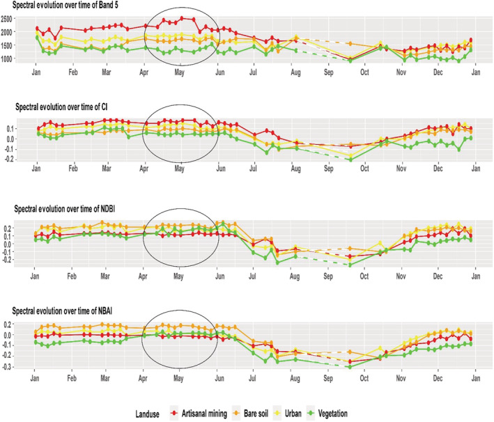
Spectral evolution over time of B5, CI, NDBI, and NBAI for Kharakhena. The circled part corresponds to the period from April to June (T2).
In order to confirm or update the list of spectral indices or bands that are optimal for detection of AGSM, an analysis of the separability between classes is carried out and presented in section 4.5.
4.5. Assessment of Best Indices and Bands to Classify ASGM Sites Versus Other Classes
The efficiency of separation based on spectral bands or spectral indices may be evaluated with the “separability measure” J (Equation 2). For each class, the index with the highest value of J is interpreted as the best index. Values of J higher than 1.9 are qualified as very good separability and values between 1.5 and 1.9 are qualified as good separability. Figure 13 presents the results of the calculation of separability measures between the ASGM class and the other land use for Bantakokouta and Kharakhena. All spectral bands and indices, for the period T3 (April–June), were included in this analysis. For each figure, the horizontal axis intersects the vertical axis at the fixed threshold value of 1.5. Thus, for each band and index, the classes whose separability threshold is greater than 1.5 appear above the x axis and those whose separability is less than 1.5 appear below the x axis. For the Bantakokouta site (Figure 13a), the bands 3, 4, 5, 11, and spectral index BIa have separability measures with bare soils above the threshold value. This is explained by the presence of quartz (which constitutes the main part of mining waste) which increases the brightness of the soils. For the urban class, all separability measures are below the threshold, and therefore, confusion will remain possible in all cases. As for the water and vegetation classes, the high values of J mean that there is no possibility of confusing these classes with artisanal gold mining sites. For the Kharakhena site (Figure 13b), the BSI and CI, B4, and B5 remain the most relevant index to separate the mining site from all other classes. B6, B7, and B8 and BI can also be used to avoid confusion between the urban class, bare soil, and artisanal mining site. The indices of soil redness (RI) and the NDVI may be used to refine the classification. The most relevant variables differ between these two sites, and we can explain this by the fact that the types of land (ore zone) are different (quartz veins for Bantakokouta and lateritic duricrust for Kharakhena). We also examined the J values between bare soils and urban classes, to determine how the confusion may be avoided between these two classes. After a complete analysis of the separability between the different classes for each site, the following variables are taken as an input to our classification algorithm: B4, B5, B6, B7, B8, B8A, B11, NDVI, NDWIa, CI, BIa, NDWIb, and NDBI for Bantakokouta and B4, B5, B6, B7, B8, B11, CI, BIa, RI, BIb, and BSI for Kharakhena. The maps that are produced by the classification process are presented in section 4.6.
Figure 13.

Bantakokouta (a) and Kharakhena (b) area separability measurements between the mining site and other classes, estimated for all spectral bands and spectral indices for the period T2 (April–June). The x axis represents the spectral bands and indices and y axis the values of J.
4.6. Maps of ASGM Areas
The final classification is therefore based on the use of the set of training samples for each site and considering satellite data acquired during the period of April to June. Only bands and indices with high values of separability are used. The classification is achieved using the SVM as explained in section 3. The result of the classification was exported in tiff format into a Google Drive. The Figure 14 presents the results of the Bantakokouta (left) and Kharakhena (right) classification. Once exported, this file is opened in QGIS, and site mapping is completed manually. This step consists of doing a quality control and vector editing to eliminate major/ubiquitous misclassification of mining areas. The vector editing was straightforward and concerned only a few pixels in the villages that were clearly not related to mining sites (see Figures S4–S6). Minimal knowledge of the terrain would be required for such manual editing in other areas where automatic classification is achieved with the same performance. On the maps shown in Figure 14 (after vector editing), artisanal mining sites are labeled in red and official corridors are framed in black. The final result of this study is therefore a map of ASGM sites. By cross validating with the field reality, an overall accuracy of 0.89 is found for the Bantakokouta site (Kappa = 0.85) and 0.80 for Kharakhena (kappa = 0.73). According to the validation matrix presented in Tables 1 and 2, the mining areas are well identified (no omission error for Bantakokouta and 11% for Kharakhena) by the approach developed here. The remaining sources of confusion occur between artisanal mining sites, urban, and bare soils.
Figure 14.

Results of classification derived by the application of the SVM on selected spectral bands in indices on Sentinel 2 scenes from April to June and after manual vector editing. (left) Bantakokouta and (right) Kharakhena. Official corridors are framed in black.
Table 1.
Confusion Matrix According to Validation Data for Bantakokouta Area
| Reference data | |||||||
|---|---|---|---|---|---|---|---|
| ASGM | Bare soil | Urban | Vegetation | Water | Total | ||
| Classified Pixels? | ASGM | 289 | 2 | 5 | 0 | 0 | 296 |
| Bare soil | 0 | 489 | 29 | 0 | 0 | 518 | |
| Urban | 0 | 112 | 178 | 0 | 0 | 290 | |
| Vegetation | 0 | 28 | 0 | 335 | 0 | 363 | |
| Water | 0 | 0 | 0 | 8 | 226 | 226 | |
| Total | 289 | 631 | 212 | 343 | 226 | 1,693 | |
Note. For instance, the 212 pixels corresponding to urban areas based on field work were classified as ASGM (5 pixels), bare soils (29 pixels), and urban (178 pixels).
Table 2.
Confusion Matrix According to Validation Data for Kharakhena Area
| Reference data | ||||||
|---|---|---|---|---|---|---|
| ASGM | Bare soil | Urban | Vegetation | Total | ||
| Classified Data | ASGM | 362 | 13 | 56 | 0 | 431 |
| Bare soil | 18 | 319 | 62 | 4 | 403 | |
| Urban | 27 | 66 | 282 | 0 | 375 | |
| Vegetation | 4 | 52 | 4 | 288 | 348 | |
| Total | 411 | 450 | 404 | 292 | 1,557 | |
Note. For instance, the 411 pixels corresponding to ASGM based on field work were classified as ASGM (362 pixels), bare soils (18 pixels), urban (27 pixels), and vegetation (4 pixels).
Once these results are obtained, we can perform a vector editing and extract only the gold mining sites. All areas erroneously classified as ASGM are erased after vectorization. This step depends on our knowledge of the terrain and the validation step.
5. Discussion
Considering that until now, no methodology has been developed for monitoring artisanal gold mining in Senegal; this research proposes a fast, robust, and inexpensive technique for accurate identifying and mapping sites. This methodology is adapted to the context of developing countries by focusing on free data (Sentinel 2), open access software (R and QGIS), and cloud computing (GEE). The selection and download of Sentinel 2 data that would take a long time is avoided by the cloud computing alternative option on the GEE Platform. The calculation and extractions of the spectral information and the results of the calculations can be obtained in a few minutes. (This only includes computation time, not the time for the analyses of separability and threshold results and selection of spectral bands and indices.) This represents a decisive advantage in a context where there are limited computing resources and internet bandwidth dedicated to such applications.
The methodology relies on a series of statistical methods that can be implemented elsewhere in West Africa, to determine, in each particular case, the optimal period of the year and the optimal spectral indices or spectral bands to discriminate artisanal mining sites from other land use. Field observations are needed at the first step, but the optimized parameters may be applied to the neighboring regions with similar vegetation, land use, and climatic conditions. The separability of classes shows that soil indices such as brightness, color indices, and bare soil indices are much more relevant for identifying sites, in the context of our case of study where there is a lot of difficulty in identifying the different types of bare soil including those related to artisanal mining. The thresholds obtained with the calculation of the Jeffries‐Matusita distances can be used in case we want to automate the detection of sites. The optimal spectral parameters may partly change over short distance, as it was observed to be the case between Bantakokouta and Kharakhena. However, it is of note that for the neighboring sites in Eastern Senegal, the optimum period is the end of the dry season, and these results are probably valid for the Sahelian region characterized by one rainy season. The fact that the end of the dry season is the best to identify mining site appears to be the confirmation of an intuitive result; as for the geologist, the vegetation cover during the rainy season is generally an obstacle to discriminate between geology units; the same would apply to the capacity to discriminate between other types of land use.
As mentioned in section 1, remote sensing has been used since 2004 in West Africa (Kusimi, 2008; Manu et al., 2004; Obodai et al., 2019; Snapir et al., 2017) but these studies were all focused on Ghanaian mining sites and used pre‐Sentinel imagery. The approaches used in these studies share similarities: use of time series, supervised classification, calculation of vegetation loss, mapping extent and expansion of ASGM, land use and land cover change etc. The locations of Ghana's mining districts are well known, which can facilitate the detection of change over several years over large areas. The novel aspects of this study with respect to previous ones are as follows: the application to mining sites in Senegal, in a region with Sahelian climate, rather than tropical climate, the use of Sentinel data (more frequent images, larger number of spectral channel with high resolution), and the application to small mining sites.
Snapir et al. (2017) are the only study to our knowledge that used UK‐DMC2, a multispectral imaging satellite operating in green, red and near infrared at 22 m resolution (better than Landsat resolution) to map the extent and expansion of illegal gold mining from 2011 to 2015. This study could be completed by using the Sentinel 2 data available since the end of 2015, taking advantage of the extended multispectral capabilities and resolution (pixel size of 10 m). It is of note that other classification approaches are possible such as maximum likelihood, minimum distance and spectral angle mapper. For instance, Obodai et al. (2019) and Boakye et al. (2020) used the spectral angle mapper in Ghana. The performance of this classification methods has been qualitatively estimated in our ROI, and we found that these alternative approaches do not surpass the SVM classifier (see Figures S7 and S8). Indeed, this study demonstrates the added value of including spectral indices in addition to spectral band.
Extrapolation of these results to tropical areas, for instance, in Southern Ghana, Guinea, and Côte d'Ivoire where artisanal mining activities are also important. At this stage, it is not clear which part of the year would be the best to identify mining sites in these regions, although all of the studies cited were done with data acquired in dry season, to avoid cloud coverage. The high frequency of sentinel acquisition would certainly allow to analyze scenes acquired during the rainy seasons (with occasional cloud‐free skies) to apply our quantitative approach to determine the best season for mapping ASGM sites. New field observations would be necessary to adapt the current method to these sites, but an overall similar methodology could be applied. Recently, Forkuor et al. (2020) used Sentinel 1 data (radar) for mapping and monitoring small‐scale mining activities in Ghana (2015–2019). An approach based on detection of surface properties modifications has allowed the detection of new illegal sites on an annual basis at the beginning and end of the rainy season. This approach can be combined with optical imagery in future studies to continue monitoring ASGM areas even during the rainy season. The use of higher resolution optical data (Pleiades, planet) or Radar (Radarsat‐2, CosmoSkymed, ALOS‐2) can be considered for more precise site detection (especially new sites in the early stages of formation).
Also, the classification which can take a lot of time with GIS software is done very quickly on GEE. SVM has many advantages because it can complete an accurate classification with little training data. However, the very low separability index found between urban and bare soil means that there is always a risk of confusion influencing our global kappa (validation) index.
This methodology can be easily automated for the detection of other artisanal gold mining sites. Once detected, these sites can be vectorized and these vectors can feed a GIS database where all the necessary information for the follow‐up of the gold mining would be included. It should also be noted that once detected, the sites could be superimposed on the legal perimeters, which would allow the authorities in charge of monitoring this activity to better localize legal and clandestine activities. Some legal sites also extend beyond the permits and become illegal, hence the need for decision makers to better review the areas granted for artisanal mining. Assuming that it always exists at least one appropriate and optimal period of the year to identify artisanal mining sites, it is possible to initiate a database of mining site maps with a 1 year step between two consecutive maps.
6. Conclusion
This article presents a method for detecting and mapping ASGM sites in eastern Senegal. It is based on the use of Sentinel 2 data, GEE cloud computing, and multivariate statistical methods. The method requires two sessions of field work for collecting training samples and validation data. The novel aspects of this research are the mapping of small mining sites in Senegal and the use of Sentinel 2 time series and statistical methods to determine the optimal period of the year and the most efficient bands or spectral indices for mapping ASGM sites. With respect to the current issues with the regulation of artisanal mining in Senegal, this study provides a solution to build objective knowledge regarding the past and recent development around legal and illegal artisanal mining sites in Senegal. Finally, this study could stimulate the development of similar cost‐effective approaches in other West African countries facing the same challenges for the monitoring and regulation of artisanal gold mining activities.
Conflict of Interest
The authors declare no conflicts of interest relevant to this study.
Supporting information
Supporting Information S1
Acknowledgments
This research was developed in a partnership between the University Cheikh Anta Diop of Senegal (UCAD) and the UMR 228 ESPACE‐DEV (Maison de la Télédétection) of Montpellier (France). The authors would like to acknowledge financial support from the French National Research Institute for Sustainable Development (IRD, LMI MINERWA Laboratory for Responsible Mining in West Africa) and the French embassy in Senegal which supported the lead author as part of her PhD research project. N. M. N. received a PhD grant from the Ministry of Higher Education and Research and Innovation of the Republic of Senegal. We thank the two anonymous reviewers for their critical comments which helped us significantly to improve the manuscript.
Ngom, N. M. , Mbaye, M. , Baratoux, D. , Baratoux, L. , Catry, T. , Dessay, N. , et al. (2020). Mapping artisanal and small‐scale gold mining in Senegal using Sentinel 2 data. GeoHealth, 4, e2020GH000310 10.1029/2020GH000310
Data Availability Statement
Data supporting our conclusions can be obtained from the Open Science Framework website (https://osf.io/k7enc/quickfiles).
References
- Agence Nationale de la Statistique et de la Démographie (2018). Rapport de l'étude Monographique Sur l'orpaillage Au Sénégal. Sénégal: ANSD; http://www.ansd.sn/ressources/rapports/RAPPORT_EMOR_du_20_juillet_2018.pdf [Google Scholar]
- Ako, T. A. , Onoduku, U. S. , Adamu, I. A. , Ali, S. E. , Mamodu, A. , & Ibrahim, A. T. (2014). Environmental impact of artisanal gold mining in Luku, Minna, Niger State, North Central Nigeria. Journal of Geosciences and Geomatics, 2(1), 28–37. 10.12691/jgg-2-1-5 [DOI] [Google Scholar]
- Aryee, B. , Bernard, N. A. , Ntibery, K. , & Atorkui, E. (2003). Trends in the small‐scale mining of precious minerals in Ghana: A perspective on its environmental impact. Journal of Cleaner Production, 11(2), 131–140. 10.1016/S0959-6526(02)00043-4 [DOI] [Google Scholar]
- Bakia, M. (2014). East Cameroon's artisanal and small‐scale mining bonanza: How long will it last? Futures, 62, 40–50. 10.1016/j.futures.2013.10.022 [DOI] [Google Scholar]
- Bamba, O. , Pelede, S. , Sako, A. , Kagambega, N. , & Miningou, M. Y. W. (2013). Impact de l'artisanat minier sur les sols d'un environnement agricole amenage au Burkina Faso 13: 12.
- Banko, G. (1998). A review of assessing the accuracy of classifications of remotely sensed data and of methods including remote sensing data in forest inventory. IIASA Interim Report IR‐98‐081. Laxenburg, Austria: IIASA. http://pure.iiasa.ac.at/5570/
- Boakye, E. , Anyemedu, F. O. K. , Quaye‐Ballard, J. A. , & Donkor, E. A. (2020). Spatio‐temporal analysis of land use/cover changes in the Pra River Basin, Ghana. Applied Geomatics, 12(1), 83–93. 10.1007/s12518-019-00278-3 [DOI] [Google Scholar]
- Boudou, A. , Dominique, Y. , Cordier, S. , & Frery, N. (2006). Les Chercheurs d'or et La Pollution Par Le Mercure En Guyane Française: Conséquences Environnementales et Sanitaires. Environnement, Risques & Santé, 5(n° 3), 14. [Google Scholar]
- Bruzzone, L. , Chi, M. , & Marconcini, M. (2006). A novel transductive SVM for Semisupervised classification of remote‐sensing images. IEEE Transactions on Geoscience and Remote Sensing, 44(11), 3363–3373. 10.1109/TGRS.2006.877950 [DOI] [Google Scholar]
- Buxton, A. (2013). Responding to the challenge of artisanal and small‐scale mining. How can knowledge networks help? London: IEED; https://pubs.iied.org/pdfs/16532IIED.pdf [Google Scholar]
- Diop, C. T. (2008). Recensement Des Sites d'orpaillage Dans Les Régions de Kédougou et Tambacounda, Sénégal. Direction des Mines et de la Géologie du Sénégal.
- Elmes, A. , Gabriel Yarlequé Ipanaqué, J. , Rogan, J. , Cuba, N. , & Bebbington, A. (2014). Mapping licit and illicit mining activity in the Madre de Dios Region of Peru. Remote Sensing Letters, 5(10), 882–891. 10.1080/2150704X.2014.973080 [DOI] [Google Scholar]
- Eludoyin, A. O. , Ojo, A. T. , Ojo, T. O. , & Awotoye, O. O. (2017). Effects of artisanal gold mining activities on soil properties in a part of southwestern Nigeria. Edited by Thaddeus Nzeadibe. Cogent Environmental Science, 3(1), 1305650 10.1080/23311843.2017.1305650 [DOI] [Google Scholar]
- Foody, G. M. , & Mathur, A. (2004). Toward intelligent training of supervised image classifications: Directing training data acquisition for SVM classification. Remote Sensing of Environment, 93(1–2), 107–117. 10.1016/j.rse.2004.06.017 [DOI] [Google Scholar]
- Forkuor, G. , Ullmann, T. , & Griesbeck, M. (2020). Mapping and monitoring small‐scale mining activities in Ghana using Sentinel‐1 time series (2015–2019). Remote Sensing, 12(6), 911 10.3390/rs12060911 [DOI] [Google Scholar]
- Gerson, J. R. , Driscoll, C. T. , Hsu‐Kim, H. , & Bernhardt, E. S. (2018). Senegalese artisanal gold mining leads to elevated total mercury and methylmercury concentrations in soils, sediments, and rivers. Elementa Science of Anthropocene, 6(1), 11 10.1525/elementa.274 [DOI] [Google Scholar]
- Gond, V. , & Brognoly, C. (2005). Télédétection et aménagement du territoire: localisation et identification des sites d'orpaillage en Guyane française. Bois et Forêts des tropiques, 286(4), 5–13. [Google Scholar]
- Hilson, G. (2002). Harvesting mineral riches: 1000 years of gold mining in Ghana. Resources Policy, 28(1–2), 13–26. 10.1016/S0301-4207(03)00002-3 [DOI] [Google Scholar]
- Hilson, G. (2008). A load too heavy: Critical reflections on the child labor problem in Africa's small‐scale mining sector. Children and Youth Services Review, 30(11), 1233–1245. 10.1016/j.childyouth.2008.03.008 [DOI] [Google Scholar]
- Hilson, G. (2009). Small‐scale mining, poverty and economic development in sub‐Saharan Africa: An overview. Resources Policy, 34(1–2), 1–5. 10.1016/j.resourpol.2008.12.001 [DOI] [Google Scholar]
- Hilson, G. (2010). Child labour in African artisanal mining communities: Experiences from northern Ghana: Child labour in artisanal mining communities (northern Ghana). Development and Change, 41(3), 445–473. 10.1111/j.1467-7660.2010.01646.x [DOI] [Google Scholar]
- Husson, F. , Lê, S. , & Pagès, J. (2017). Exploratory Multivariate Analysis by Example Using R. 13 978‐1‐1381‐9634–6. New York: Taylor & Francis Group, LLC. [Google Scholar]
- Ifarraguerri, A. , & Prairie, M. W. (2004). Visual method for spectral band selection. IEEE Geoscience and Remote Sensing Letters, 1(2), 101–106. 10.1109/LGRS.2003.822879 [DOI] [Google Scholar]
- Isidro, C. M. , McIntyre, N. , Lechner, A. M. , & Callow, I. (2017). Applicability of earth observation for identifying small‐scale mining footprints in a wet tropical region. Remote Sensing, 9(9), 945 10.3390/rs9090945 [DOI] [Google Scholar]
- Kassambara (2017). Articles—Méthodes des composantes principales Dans R: Guide pratique. Statistical Tools For High‐Throughput Data Analysis. 2017. http://www.sthda.com/french/articles/38-methodes‐des‐composantes‐principales‐dans‐r‐guide‐pratique/73‐acp‐analyse‐en‐composantes‐principales‐avec‐r‐l‐essentiel/
- Kitula, A. G. N. (2006). The environmental and socio‐economic impacts of mining on local livelihoods in Tanzania: A case study of Geita District. Journal of Cleaner Production, 14(3–4), 405–414. 10.1016/j.jclepro.2004.01.012 [DOI] [Google Scholar]
- Kusimi, J. M. (2008). Assessing land use and land cover change in the Wassa West District of Ghana using remote sensing. GeoJournal, 71(4), 249–259. 10.1007/s10708-008-9172-6 [DOI] [Google Scholar]
- LaJeunesse Connette, K. , Connette, G. , Bernd, A. , Phyo, P. , Aung, K. , Tun, Y. , Thein, Z. , Horning, N. , Leimgruber, P. , & Songer, M. (2016). Assessment of mining extent and expansion in Myanmar based on freely‐available satellite imagery. Remote Sensing, 8(11), 912 10.3390/rs8110912 [DOI] [Google Scholar]
- Laperche, V. , Nontanovanh, M. , & Thomassin, J. F. (2008). Synthèse Critique Des Connaissance s Sur Les Conséquences Environne,Entqtles de l'orpaillage En Guyanes. BRGM/RP‐56652‐FR. http://infoterre.brgm.fr/rapports/RP‐56652‐FR.pdf
- Le Billon, P. (2006). Fatal transactions: Conflict diamonds and the (anti)terrorist consumer. Antipode, 38(4), 778–801. 10.1111/j.1467-8330.2006.00476.x [DOI] [Google Scholar]
- Le Billon, P. (2008). Diamond wars? Conflict diamonds and geographies of resource wars. Annals of the Association of American Geographers, 98(2), 345–372. 10.1080/00045600801922422 [DOI] [Google Scholar]
- Lewis, H. G. , & Brown, M. (2001). A generalized confusion matrix for assessing area estimates from remotely sensed data. International Journal of Remote Sensing, 22(16), 3223–3235. 10.1080/01431160152558332 [DOI] [Google Scholar]
- Lobo, F. (2015). Spatial and temporal analysis of water siltation caused by artisanal small‐scale gold mining in the Tapajós Water Basin, Brazilian Amazon: An optics and remote sensing approach. Ph.D., University of Victoria. 10.13140/RG.2.1.4455.6247 [DOI]
- Lobo, F. , Costa, M. , Novo, E. , & Telmer, K. (2016). Distribution of artisanal and small‐scale gold mining in the Tapajós River Basin (Brazilian Amazon) over the past 40 years and relationship with water siltation. Remote Sensing, 8, 579 10.3390/rs8070579 [DOI] [Google Scholar]
- Lobo, F. d. L. , de Moraes Novo, E. M. L. , Barbosa, C. C. F. , & de Vasconcelos, V. H. F. (2018). Monitoring water siltation caused by small‐scale gold mining in Amazonian Rivers using multi‐satellite images. Limnology ‐ Some New Aspects of Inland Water Ecology. 10.5772/intechopen.79725 [DOI] [Google Scholar]
- MacDonald, K. (2006). Artisanal and small‐scale mining in West Africa: Achieving sustainable development through environmental and human rights law In Hilson G. (Ed.), Chap 7Small‐Scale Mining, Rural Subsistence and Poverty in West Africa, edited by (pp. 75–101). Rugby, Warwickshire, United Kingdom: Practical Action Publishing; 10.3362/9781780445939 [DOI] [Google Scholar]
- Mantero, P. , Moser, G. , & Serpico, S. B. (2005). Partially supervised classification of remote sensing images through SVM‐based probability density estimation. IEEE Transactions on Geoscience and Remote Sensing, 43(3), 559–570. 10.1109/TGRS.2004.842022 [DOI] [Google Scholar]
- Manu, A. , Twumasi, Y. A. , & Coleman, T. L. (2004). Application of remote sensing and GIS technologies to assess the impact of surface Mining at Tarkwa, Ghana In IGARSS 2004. 2004, IEEE International Geoscience and Remote Sensing Symposium. 1:572–74. Anchorage, AK, USA: IEEE. 10.1109/IGARSS.2004.1369091 [DOI]
- Mathur, A. , & Foody, G. M. (2008). Crop classification by support vector machine with intelligently selected training data for an operational application. International Journal of Remote Sensing, 29(8), 2227–2240. 10.1080/01431160701395203 [DOI] [Google Scholar]
- Mhangara, P. , Tsoeleng, L. T. , & Mapurisa, W. (2020). Monitoring the development of artisanal mines in South Africa. Journal of the Southern African Institute of Mining and Metallurgy, 120(4). 10.17159/2411-9717/938/2020 [DOI] [Google Scholar]
- Niane, B. , Guedron, S. , Feder, F. , Legros, S. , Ngom, P. M. , & Moritz, R. (2019). Impact of recent artisanal small‐scale gold mining in Senegal: Mercury and methylmercury contamination of terrestrial and aquatic ecosystems. Science of the Total Environment, 669, 32 10.1016/j.scitotenv.2019.03.108 [DOI] [PubMed] [Google Scholar]
- Nussbaum, S , Niemeyer, I. , & Canty, M. J. (2006). SEATH—A new tool for automated feature extraction in the context of object‐based image analysis.” In, XXXVI:7. Salzburg.
- Obodai, J. , Adjei, K. A. , Odai, S. N. , & Lumor, M. (2019). Land use/land cover dynamics using Landsat data in a gold mining basin—The Ankobra, Ghana. Remote Sensing Applications: Society and Environment, 13(January), 247–256. 10.1016/j.rsase.2018.10.007 [DOI] [Google Scholar]
- Persaud, W. , Anthony, K. T. , Costa, M. , & Moore, M.‐L. (2017). Artisanal and small‐scale gold mining in Senegal: Livelihoods, customary authority, and formalization. Society & Natural Resources, 30, 1–14. 10.1080/08941920.2016.1273417 [DOI] [Google Scholar]
- Prause, L. (2016). West Africa's golden future? Conflicts around gold mining in Senegal. Natural Resources, 2016. [Google Scholar]
- Rahm, J. B. , Lauger, A. , de Carvalho, R. , Vale, L. , Totaram, J. , Cort, K. A. , Djojodikromo, M. , Hardjoprajitno, M. , Neri, S. , Vieira, R. , Watanabe, E. , do Carmo Brito, M. , Miranda, P. , Paloeng, C. , Moe Soe Let, V. , Crabbe, S. , & Calmel, M. (2014). Monitoring the impact of gold mining on the forest cover and freshwater in the Guiana shield. REDD + for the Guiana shield Project and WWf Guianas. Retrieved from https://www.wwf.fr/sites/default/files/doc‐2017‐10/1708_Rapport_Gold_mining_on_the_forest_cover_and_freshwater_in_the_Guiana_shield2.pdf
- Schueler, V. , Kuemmerle, T. , & Schröder, H. (2011). Impacts of surface gold mining on land use systems in Western Ghana. Ambio, 40(5), 528–539. 10.1007/s13280-011-0141-9 [DOI] [PMC free article] [PubMed] [Google Scholar]
- Snapir, B. , Simms, D. M. , & Waine, T. W. (2017). Mapping the expansion of galamsey gold mines in the cocoa growing area of Ghana using optical remote sensing. International Journal of Applied Earth Observation and Geoinformation, 58, 225–233. 10.1016/j.jag.2017.02.009 [DOI] [Google Scholar]
- Tourneau, F‐M. L. , & Albert, B. (2005). Sensoriamento remoto num contexto multidisciplinar: Atividade garimpeira, agricultura ameríndia e regeneração natural na Terra Indígena Yanomami (Roraima). In Anais do XII Symposium Brasileiro de Sensoriamento Remoto, 583–591.
Associated Data
This section collects any data citations, data availability statements, or supplementary materials included in this article.
Supplementary Materials
Supporting Information S1
Data Availability Statement
Data supporting our conclusions can be obtained from the Open Science Framework website (https://osf.io/k7enc/quickfiles).