

Abstract
When estimating causal effects, careful handling of missing data is needed to avoid bias. Complete-case analysis is commonly used in epidemiologic analyses. Previous work has shown that covariate-stratified effect estimates from complete-case analysis are unbiased when missingness is independent of the outcome conditional on the exposure and covariates. Here, we assess the bias of complete-case analysis for adjusted marginal effects when confounding is present under various causal structures of missing data. We show that estimation of the marginal risk difference requires an unbiased estimate of the unconditional joint distribution of confounders and any other covariates required for conditional independence of missingness and outcome. The dependence of missing data on these covariates must be considered to obtain a valid estimate of the covariate distribution. If none of these covariates are effect-measure modifiers on the absolute scale, however, the marginal risk difference will equal the stratified risk differences and the complete-case analysis will be unbiased when the stratified effect estimates are unbiased. Estimation of unbiased marginal effects in complete-case analysis therefore requires close consideration of causal structure and effect-measure modification.
Keywords: complete-case analysis, conditional estimates, epidemiologic methods, heterogeneity, marginal estimates, missing data, risk differences
Abbreviations
- CCA
complete-case analysis
- DAG
directed acyclic graph
- RD
risk difference
When estimating causal effects, careful handling of missing data is needed to avoid bias. Complete-case analysis (CCA), also known as listwise deletion (1), uses only the data records without missing values for any variable needed for analysis. CCA is the default method of several commonly used statistical packages, including SAS (SAS Institute, Inc., Cary, North Carolina) and many R packages (R Foundation for Statistical Computing, Vienna, Austria), and it is frequently used in epidemiologic analyses. Before conducting CCA, it is important to understand whether it will yield a valid estimate of the effect that the study aims to measure.
Missing data are often classified by the dependency of the missingness on measured and unmeasured data (2, 3). Data are “missing completely at random” when the probability of missingness is independent of all measured and unmeasured data. Data are “missing at random” when the missingness is independent of the unmeasured data conditional on measured data and are “missing not at random” when missingness is dependent on the unmeasured data. It is well accepted that CCA is valid when data are missing completely at random (2, 3). CCA may also be valid under some circumstances when data are missing at random and missing not at random; this is because the validity depends on the association of the outcome and missingness as generated by the underlying causal structure (1, 3–11). Specifically, when the outcome ( ) is independent of missingness (
 for completely observed) conditional on exposure (
 ) and measured covariates (
 ), then
  and CCA is expected to be valid. The parameters of the conditional mean function
  can be estimated in a number of ways, including regression analysis. However, in such a regression analysis the model specification may have important implications. This is critical, as many findings in the literature regarding the potential bias of CCA apply to stratum-specific (or stratified) effects (such as those obtained from a saturated regression model) but not necessarily (for example) those obtained from a main-effects regression model. For example, under heterogeneity, the conditions of Daniel et al. (8) ensure that
  but will not in general ensure that the association between
  and
and  (
( in the following) estimated with a main-effects model
  equals the association between
  and
and  unconditional on
  . While it is standard to refer to all effects estimated from a regression model as “conditional,” this term does not distinguish between the stratified conditional estimates and a conditional estimate (a weighted average) from the main-effects model. Therefore, to avoid this ambiguity, we will in general specifically use the term stratified or stratum-specific.
Previous work examining the validity of CCA has focused on estimating stratified effects and has largely ignored estimation of an adjusted marginal effect (i.e., an effect standardized to the covariate distribution of the study sample before any missing data). Marginal effects arguably inform public health and policy more readily than stratified effects and are the effects typically estimated by randomized trials (12). Closely related, simulations assessing the validity of CCA have rarely considered effect-measure modification (4–7, 10, 11), the presence of which would produce a marginal effect that is different from the stratified effects regardless of effect-measure collapsibility (13).
In this paper, our objective is to assess the statistical consistency of CCA for marginal effect measures under various causal structures of missingness. We specifically focus on estimation of the marginal risk difference (RD) in scenarios where stratified effect estimates are unbiased.
FRAMEWORK FOR DISCUSSION
Suppose that we have enrolled participants in a study (our study sample) with the objective of estimating the causal effect of binary exposure  on binary outcome
  in a target population from which our study sample was randomly selected (14). An individual causal effect can be expressed as
  , where subjects are indexed by
  and
and  is the outcome that would have occurred if the subject had, possibly counter to fact, experienced exposure at level
  (15). We assume that the subjects are independent and identically distributed, and for notational simplicity we drop the subject-level index,
  , hereafter. The sample average causal effect is
  (15).
(15).
In the complete data, the effect of  on
on  is confounded by a single binary variable
  (see the causal directed acyclic graph (DAG) in Figure 1) (16). We assume that accounting for
  is sufficient to achieve conditional exchangeability between exposure groups (15). We further assume positivity (all subjects in either stratum of
  have nonzero probabilities of being exposed and unexposed) (17), causal consistency (the observed outcome under exposure
  is equal to the potential outcome
  ) (18), and no measurement error (19).
Figure 1.
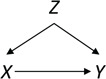
Direct acyclic graph without missing data.  , exposure;
  , outcome;
  , confounder.
We will estimate the RD nonparametrically using a standardization approach that is equivalent to nonparametric g-computation (i.e., the g-formula; see Hernán and Robins (15), part 2, pp. 23–27). This estimator provides a clear illustration of how bias can arise in CCA. Under the previously stated identification conditions, the average causal effect of  on
on  can be expressed in terms of observable quantities, specifically
 |
To obtain the standardized marginal RD in our study sample, we can apply this standardization formula to the observed data from our study. Table 1 shows a general form of the  -stratified 2 × 2 tables from the study sample. In the table,
  is the number of exposed (
 ) subjects with the outcome (
 ) without confounder
  (
( ) and
) and  is the number of exposed subjects with the outcome with confounder
  (
( ). Applying the notation from Table 1 to our standardization formula, we obtain
 |
(1) |
Table 1.
Stratified 2 × 2 Tables From the Full Study Samplea
| X |
Y  1 1 |
Y  0 0 |
Total |
|---|---|---|---|

| |||

|

|

|

|

|

|

|

|
| Total |

|

|

|

| |||

|

|

|

|

|

|

|

|
| Total |

|

|

|
a X, exposure; Y, outcome; Z, confounder.
We observe that the marginal RD can be expressed as the weighted average of the stratum-specific RDs. Specifically, each stratum-specific RD is weighted by the proportion of the population with that value of  . Therefore, in order to obtain the equivalent RD from CCA, we must obtain valid estimates of both the stratum-specific RDs and the distribution of
  from the study sample. One important exception to this is that if the 2 stratum-specific RDs are identical (homogenous on the absolute scale), then we do not need the distribution of
  , because any weighted average of the two will yield the correct marginal RD; that is,
  . Therefore, the distribution of
  will not affect the marginal RD when
  is not an effect-measure modifier. However, because
  is a cause of
  (Figure 1), when there is a nonnull effect of
  on
on  and of
  on
on  , there will be effect-measure modification by
  on at least 1 scale (either absolute or relative) (14). For example, if the RD for the effect of
  on
on  is the same regardless of the value of
  , the risk ratio will be different by the value of
  (though we may lack the statistical power to detect this in real data). Thus, even if the distribution of
  in the study sample is not needed to obtain a valid marginal RD, the distribution will generally be required to obtain a valid risk ratio (and vice versa).
MISSING DATA AND COMPLETE-CASE ANALYSIS
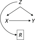
Now we introduce missing data to the DAG by including an additional node,  , which is an indicator of missingness (Figure 2). We use
  to indicate participants for whom the full data are observed and
  for participants with missing data on at least 1 variable among the exposure, outcome, or confounder. CCA is an analysis conditional on (restricted to)
  , which is depicted in Figure 2 by a box around
  .
.
Figure 2.
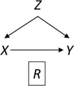
Causal diagram for data missing completely at random.  , missing-data indicator;
  , exposure;
  , outcome;
  , confounder.
As outlined above, to validly estimate the marginal RD, CCA must provide valid estimates of both 1) the stratum-specific RDs and 2) the distribution of Z from the study sample. First, the stratum-specific RDs conditional on  will equal the stratum-specific RDs in the study sample (unconditional on
  ),
),
 |
when  is independent of
  conditional on
  and
and  . This condition has been previously described in the literature (1, 3–11) and in the Introduction above. Second, the distribution of confounder
  conditional on
  will equal the distribution in the study sample,
  , when
  is independent of
  . In the remainder of this paper, we pay particular attention to this condition. This condition is sufficient; however, it is not necessary when
  does not modify the effect of
  on
on  on the scale of interest (homogeneity).
Data missing completely at random
Figure 2 depicts the causal structure in which data are missing completely at random, since  is independent of other nodes on the DAG. If the probability that we observe complete data (
 ) is
) is  and we conduct a CCA, we obtain new stratified 2 × 2 tables (Table 2). Using these new data tables and formula 1 above, the marginal RD estimate is
 |
Table 2.
Stratified 2 × 2 Tables From a Complete-Case Analysis in Which Data Are Missing Completely at Randoma,b
| X |
Y  1 1 |
Y  0 0 |
Total |
|---|---|---|---|

| |||

|

|

|

|

|

|

|

|
| Total |

|

|

|

| |||

|

|

|

|

|

|

|

|
| Total |

|

|

|
a The table reflects the structure of missingness shown in Figure 2.
b f, probability that complete data are observed; X, exposure; Y, outcome; Z, confounder.
We observe that  cancels out in the stratum-specific RDs,
 |
and the distribution of  . These equalities hold because in Figure 2
  is independent of
  and
and  , respectively. Because the stratum-specific RDs and the distribution of
  are identifiable, the marginal RD obtained from CCA is a valid estimate of the marginal RD in the study sample.
Missingness caused by a confounder
Figure 3 depicts confounder  as the cause of missingness. In these simple DAGs, the causal structure does not dictate which data elements are missing. Confounder
  causes
  , but
, but  represents missing data for any data element, so the DAG does not distinguish between data that are missing at random and data that are missing not at random. In Figure 3, data are missing at random if only exposure or outcome data were missing; data are missing not at random if confounder data were missing.
Figure 3.
Causal diagram for missingness caused by a confounder.  , missing-data indicator;
  , exposure;
  , outcome;
  , confounder.
Considering Figure 3, if the probability that we observe complete data ( ) is
) is  for subjects with Z = 0 and
  for subjects with
  and we conduct a CCA, we would obtain new stratified 2 × 2 tables (Table 3). Using these tables and formula 1, the marginal RD estimate is
 |
Table 3.
Stratified 2 × 2 Tables From a Complete-Case Analysis in Which Missing Data Are Caused by a Confoundera,b
| X |
Y  1 1 |
Y  0 0 |
Total |
|---|---|---|---|

| |||

|

|

|

|

|

|

|

|
| Total |

|

|

|

| |||

|

|

|

|

|

|

|

|
| Total |

|

|

|
a The table reflects the structure of missingness shown in Figure 3.
b f, probability that complete data are observed when  ; g, probability that complete data are observed when
  ; X, exposure; Y, outcome; Z, confounder.
We observe that  and
and  cancel out of the stratum-specific RDs:
 |
and
 |
This equality holds because in Figure 3,  is independent of
  conditional on
  (
( ). However, the estimated distribution of
  is no longer a valid estimate of the unconditional distribution of
  in the study sample:
  . In Figure 3, we observe that
  is not independent of
  because there is a path from
  to
to  and therefore
  .
.
Since the estimate of the  distribution from CCA is not valid, the marginal RD will not be a valid estimate of the marginal RD in the study sample, except when the effect of
  on
on  is homogeneous across strata of
  on the absolute scale. If the RD is homogeneous by
  , we would likely not be able to obtain the valid marginal risk ratio, however, because the risk ratio will not be homogeneous (unless there is a null effect of
  on
on  in both strata of
  ). If
). If  data are not missing and are therefore available in the full data, we can apply the fully observed study sample distribution of
  to the stratum-specific estimates from CCA to recover the valid marginal RD. If
  data are missing, we may be able to recover the distribution of
  by multiple imputation or weighting (20).
If there were not an arrow from  to
to  ,
,  would not be a confounder and we would no longer need to control for
  to remove confounding. However, in such a case, conditioning on
  might still be required to block the path between
  and
and  (the first condition discussed above) in order to obtain unbiased stratified effect estimates. Here,
  is sometimes called an auxiliary variable (21), a variable that is not a confounder but is nonetheless necessary for conditional independence of missingness and outcome. When we condition on
  , we will need a valid estimate of the distribution of
  to estimate the marginal effect. Therefore, the unconditional independence of
  and
and  also applies to auxiliary variables.
Missingness caused by exposure
Figure 4A depicts exposure as the cause of missingness. If the probability that we observe the complete data ( ) is
) is  for subjects with exposure
  and
and  for subjects with exposure
  and we conduct a CCA, we obtain new stratified 2 × 2 tables (Table 4). Using these tables and formula 1, the marginal RD is
 |
Figure 4.
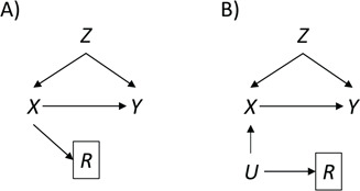
Causal diagrams for missingness associated with exposure. A) Exposure causes missingness; B) exposure and missingness have a common cause.  , missing-data indicator;
  , common cause of exposure and missingness;
  , exposure;
  , outcome;
  , confounder.
Table 4.
Stratified 2 × 2 Tables From a Complete-Case Analysis in Which Missing Data Are Caused by Exposurea,b
| X |
Y  1 1 |
Y  0 0 |
Total |
|---|---|---|---|

| |||

|

|

|

|

|

|

|

|
| Total |

|

|

|

| |||

|

|

|

|

|

|

|

|
| Total |

|

|

|
a The table reflects the structure of missingness shown in Figure 4A.
b f, probability that complete data are observed when  ; g, probability that complete data are observed when
  ; X, exposure; Y, outcome; Z, confounder.
Again,  and
and  cancel out of the stratum-specific RDs:
  . This equality holds because in Figure 4A,
  is independent of
  conditional on
  . Conditioning on
  blocks both paths from
  to
to  and
and  ). We must also condition on
  because it is a confounder. The estimate of the distribution of
  , however, is biased,
 |
because there is an open path from  to
to 
 . Analysis generally would condition on
  ; one might expect that conditioning on
  would block this path, but this is not sufficient. We need to recover the unconditional distribution of
  , not the distribution of
  conditional on
  . Therefore, similar to the previous example (Figure 3), the marginal RD from CCA will not be a valid estimate of the marginal RD in the study sample, except in the case of homogeneity over
  on the absolute scale.
To gain further understanding of how we can use the causal diagram to determine whether the distribution of  is altered in CCA, we examine a new DAG (Figure 4B). A new node
  , which is a common cause of
  and
and  , is added. Under this causal structure, the distribution of
  in CCA is unbiased because
  is now a collider on the path from
  to
to  , and thus the path is not open (see Hernán and Robins (15), part 1, p. 75). In summary, if there is an open path between a variable and a missingness indicator, then, in general, the distribution of that variable (here
  ) in CCA will not be a valid estimate of the distribution in the study sample.
DISCUSSION
Epidemiology is the study of population health (22, 23), and thus estimation of population-level effects (i.e., marginal effects) is often a primary aim. Here we have shown that conclusions drawn about the validity of stratified effects from CCA in previous work (1, 3–11) may not hold for the estimation of marginal effects and that effect-measure modification plays an important role in validity.
Stratified effect estimates from CCA are consistent when missingness is independent of the outcome conditional on exposure and covariates. If the aim is to estimate effects stratified by confounders and auxiliary variables (21) required for conditional independence of missingness and the outcome, then this condition may be sufficient to conduct CCA. If, however, the aim is to estimate a marginal effect, a valid estimate of the distribution of the covariates (confounders and auxiliary variables) that are effect modifiers is needed. In the causal structures we examined, when missingness was unconditionally independent of the confounder, the estimate of the confounder distribution in CCA was valid and thus so was the marginal RD. When missingness was associated with the confounder, the confounder distribution estimate was not valid in CCA and the marginal RD estimate was biased, except when the effect was homogeneous over the confounder on the absolute scale. Note that the marginal risks (as opposed to contrasts in risks) will be biased when the distribution of confounders and auxiliary variables is biased, regardless of modification. While our illustration uses standardization, estimation via inverse probability weighting would be expected to behave similarly.
We have focused on estimation of marginal effects, which is a contrast of the weighted average of the covariate-stratified risks weighted by the proportion of the population in each stratum. In much of the applied epidemiologic literature, however, it is common practice to obtain a single estimate of the effect of an exposure on an outcome from a main-effects regression. This conditional estimate is a statistical information-weighted average of the covariate-stratified effects. When the covariate distribution is altered in CCA, the statistical information provided by each stratum is also likely to be altered. Our conclusions, therefore, are expected to apply to these information-weighted average estimates obtained from main-effects models. Technically, when there is heterogeneity, a main-effects model is misspecified; however, it is common in practice to fit this model without checking the homogeneity assumption in order to produce a single effect estimate when stratified effects are not of interest.
Below we present a series of questions with responses to aid discussion of these results.
Question 1. It is known that for collapsible effect measures, stratified and marginal effects will be equal under homogeneity but will not be equal when there is effect-measure modification ( 13). What do your results add?
First, we hope that our paper provides intuition for the relationship between stratified and marginal effects to readers who may not already have that foundation. Primarily, the work highlights that for equivalence of stratified and marginal effects in CCA there must be, in general, homogeneity of the exposure effect over the distribution of confounders and auxiliary variables. When we include only records with complete data, the distribution of modifiers that is necessary for the valid estimation of a marginal effect may be altered. Our work attempts to illustrate how to use DAGs to identify whether the unconditional distribution of covariates will be biased in CCA compared with the full study sample.
Question 2. Why have you not discussed the scenario in which the outcome is a cause of missingness?
When the outcome causes missingness, stratified RDs and risk ratios are biased (9). When stratified estimates are biased, it is generally not possible to estimate a valid marginal effect. The odds ratio estimate may be unbiased; however, this work focuses on contrasts of risks. We refer readers to the paper by Daniel et al. (8), which includes a visualization of the collider bias produced when the outcome is a cause of missingness.
Question 3. Is this a discussion of internal or external validity, and how does it relate to generalizability or selection bias?
The independence of selection and effect modifiers has been largely discussed in the context of generalizability (24, 25). Generalizability is usually related to external validity asking, Does the estimate obtained from the study sample generalize to an external or larger target population? Because the aim of this work was to estimate a marginal effect in the study sample (our study target), our question was one of internal validity. The question of internal validity of CCA is analogous to generalizability asking, for example, Does the estimate obtained from the subset of records without missing data “generalize” to the study sample?
The potential bias that arises in CCA when missingness is dependent on modifiers may also be called selection bias without colliders (26). When the missingness is a direct or downstream effect of a modifier, then the missingness indicator itself is a modifier (effect modification by proxy) (27). It has been proposed that selection bias due to restricting analysis to 1 level of a modifier be called type 2 selection bias, whereas type 1 selection bias is conditioning on a collider (28).
Question 4. Have these results been illustrated before in prior work?
Daniel et al.’s algorithm (8) uses causal diagrams to determine whether stratified risks obtained from CCA are biased and includes a brief discussion of bias in marginal risks when the distribution of covariates is biased. Because work focuses on risk estimation, the potential impact of effect modification on the effect is not discussed. Causal diagrams specifically for missingness, m-graphs, have been developed (29, 30). Because our conclusions are agnostic to which variables have missing data, we have not used m-graphs. An algorithm for ascertaining the “recoverability” of effects from an m-graph has been published (31). This work builds on Bareinboim et al.’s (32) conditions for recoverability from selection bias. The importance of the dependence of missingness on an effect modifier in CCA has been illustrated in simulations by Choi et al. (33). In scenarios with effect modification, CCA was biased even when data missingness was conditionally independent of the outcome. The authors explained that the CCA estimate is valid for the full study sample only if the modifier and missing-data indicator are unconditionally independent. Our work attempts to explain this observation. Howe et al. (34) have previously discussed these concepts related to loss to follow-up and have called this selection bias. Additionally, although the simulations are focused on estimation of the odds ratio, Bartlett et al. (11) discussed these concepts under the topic of model misspecification.
Question 5. What are the implications?
Estimation of unbiased marginal effects in CCA requires close consideration of causal structure and effect-measure modification. However, the amount of bias may not be meaningful. Further work is needed to understand how the amount of missingness, the strength of dependence of missingness on modifiers, and the extent of modification influence this bias.
ACKNOWLEDGMENTS
Author affiliations: Department of Epidemiology, Gillings School of Global Public Health, University of North Carolina at Chapel Hill, Chapel Hill, North Carolina (Rachael K. Ross, Alexander Breskin, Daniel Westreich); and NoviSci, Durham, North Carolina (Alexander Breskin).
This work was supported by the Eunice Kennedy Shriver National Institute of Child Health and Human Development (grant 1DP2HD084070-01). R.K.R. was supported by the National Institute on Aging (grant R01 AG056479).
Conflict of interest: none declared.
REFRENCES
- 1. Little RJ. Regression with missing X’s: a review. J Am Stat Assoc. 1992;87(420):1227–1237. [Google Scholar]
- 2. Rubin DB. Inference and missing data. Biometrika. 1976;63(3):581–592. [Google Scholar]
- 3. Little RJ, Rubin DB. Statistical Analysis With Missing Data. New York, NY: John Wiley & Sons, Inc.; 1987. [Google Scholar]
- 4. Vach W, Blettner M. Biased estimation of the odds ratio in case-control studies due to the use of ad hoc methods of correcting for missing values for confounding variables. Am J Epidemiol. 1991;134(8):895–907. [DOI] [PubMed] [Google Scholar]
- 5. Rathouz PJ. Identifiability assumptions for missing covariate data in failure time regression models. Biostatistics. 2007;8(2):345–356. [DOI] [PubMed] [Google Scholar]
- 6. Giorgi R, Belot A, Gaudart J, et al. The performance of multiple imputation for missing covariate data within the context of regression relative survival analysis. Stat Med. 2008;27(30):6310–6331. [DOI] [PubMed] [Google Scholar]
- 7. White IR, Carlin JB. Bias and efficiency of multiple imputation compared with complete-case analysis for missing covariate values. Stat Med. 2010;29(28):2920–2931. [DOI] [PubMed] [Google Scholar]
- 8. Daniel RM, Kenward MG, Cousens SN, et al. Using causal diagrams to guide analysis in missing data problems. Stat Methods Med Res. 2012;21(3):243–256. [DOI] [PubMed] [Google Scholar]
- 9. Westreich D. Berkson’s bias, selection bias, and missing data. Epidemiology. 2012;23(1):159–164. [DOI] [PMC free article] [PubMed] [Google Scholar]
- 10. Bartlett JW, Carpenter JR, Tilling K, et al. Improving upon the efficiency of complete case analysis when covariates are MNAR. Biostatistics. 2014;15(4):719–730. [DOI] [PMC free article] [PubMed] [Google Scholar]
- 11. Bartlett J, Harel O, Carpenter JR. Asymptotically unbiased estimation of exposure odds ratios in complete records logistic regression. Am J Epidemiol. 2015;182(8):730–736. [DOI] [PMC free article] [PubMed] [Google Scholar]
- 12. Austin PC. An introduction to propensity score methods for reducing the effects of confounding in observational studies. Multivar Behav Res. 2011;46(3):399–424. [DOI] [PMC free article] [PubMed] [Google Scholar]
- 13. Mohammad K, Hashemi-Nazari SS, Mansournia N, et al. Marginal versus conditional causal effects. J Biostat Epidemiol. 2015;1(3-4):121–128. [Google Scholar]
- 14. Westreich D, Edwards JK, Lesko CR, et al. Target validity and the hierarchy of study designs. Am J Epidemiol. 2019;188(2):438–443. [DOI] [PMC free article] [PubMed] [Google Scholar]
- 15. Hernán M, Robins J. Causal Inference. (August 13, 2018, version) Boca Raton, FL: Chapman & Hall/CRC Press; In press https://www.hsph.harvard.edu/miguel-hernan/causal-inference-book/. Accessed August 28, 2020. [Google Scholar]
- 16. Greenland S, Pearl J, Robins JM. Causal diagrams for epidemiologic research. Epidemiology. 1999;10(1):37–48. [PubMed] [Google Scholar]
- 17. Westreich D, Cole SR. Invited commentary: positivity in practice. Am J Epidemiol. 2010;171(6):674–677. [DOI] [PMC free article] [PubMed] [Google Scholar]
- 18. Cole SR, Frangakis CE. The consistency statement in causal inference: a definition or an assumption? Epidemiology. 2009;20(1):3–5. [DOI] [PubMed] [Google Scholar]
- 19. Edwards JK, Cole SR, Westreich D. All your data are always missing: incorporating bias due to measurement error into the potential outcomes framework. Int J Epidemiol. 2015;44(4):1452–1459. [DOI] [PMC free article] [PubMed] [Google Scholar]
- 20. Perkins NJ, Cole SR, Harel O, et al. Principled approaches to missing data in epidemiologic studies. Am J Epidemiol. 2018;187(3):568–575. [DOI] [PMC free article] [PubMed] [Google Scholar]
- 21. Thoemmes F, Rose N. A cautious note on auxiliary variables that can increase bias in missing data problems. Multivar Behav Res. 2014;49(5):443–459. [DOI] [PubMed] [Google Scholar]
- 22. Rose G. Sick individuals and sick populations. Int J Epidemiol. 2001;30(3):427–432. [DOI] [PubMed] [Google Scholar]
- 23. Rockhill B. Theorizing about causes at the individual level while estimating effects at the population level: implications for prevention. Epidemiology. 2005;16(1):124–129. [DOI] [PubMed] [Google Scholar]
- 24. Lesko CR, Buchanan AL, Westreich D, et al. Generalizing study results: a potential outcomes perspective. Epidemiology. 2017;28(4):553–561. [DOI] [PMC free article] [PubMed] [Google Scholar]
- 25. Cole SR, Stuart EA. Generalizing evidence from randomized clinical trials to target populations: the ACTG 320 trial. Am J Epidemiol. 2010;172(1):107–115. [DOI] [PMC free article] [PubMed] [Google Scholar]
- 26. Hernán MA. Invited commentary: selection bias without colliders. Am J Epidemiol. 2017;185(11):1048–1050. [DOI] [PMC free article] [PubMed] [Google Scholar]
- 27. VanderWeele TJ, Robins JM. Four types of effect modification: a classification based on directed acyclic graphs. Epidemiology. 2007;18(5):561–568. [DOI] [PubMed] [Google Scholar]
- 28. Lu H, Cole SR, Westreich D. Toward a clearer definition of selection bias Presented at the 52nd Annual Meeting of the Society for Epidemiologic Research, Minneapolis, Minnesota, June 18–21, 2019. [Google Scholar]
- 29. Mohan K, Pearl J, Tian J. Graphical models for inference with missing data In: Burges CJC, Bottou L, Welling M, et al., eds. NIPS’13: Proceedings of the 26th International Conference on Neural Information Processing Systems. Vol. 1. Red Hook, NY: Curran Associates, Inc.; 2013:1277–1285. [Google Scholar]
- 30. Thoemmes F, Mohan K. Graphical representation of missing data problems. Struct Equ Model Multidiscip J. 2015;22(4):631–642. [Google Scholar]
- 31. Moreno-Betancur M, Lee KJ, Leacy FP, et al. Canonical causal diagrams to guide the treatment of missing data in epidemiologic studies. Am J Epidemiol. 2018;187(12):2705–2715. [DOI] [PMC free article] [PubMed] [Google Scholar]
- 32. Bareinboim E, Tian J, Pearl J. Recovering from selection bias in causal and statistical inference Presented at the 28th AAAI Conference on Artificial Intelligence, Quebec City, Quebec, Canada, July 27–31, 2014. [Google Scholar]
- 33. Choi J, Dekkers OM, Le Cessie S. A comparison of different methods to handle missing data in the context of propensity score analysis. Eur J Epidemiol. 2019;34(1):23–36. [DOI] [PMC free article] [PubMed] [Google Scholar]
- 34. Howe CJ, Cole SR, Lau B, et al. Selection bias due to loss to follow up in cohort studies. Epidemiology. 2016;27(1):91–97. [DOI] [PMC free article] [PubMed] [Google Scholar]