A novel bioinformatics approach to identify the consistently well-performing normalization strategy for current metabolomic studies

Abstract

Unwanted experimental/biological variation and technical error are frequently encountered in current metabolomics, which requires the employment of normalization methods for removing undesired data fluctuations. To ensure the ‘thorough’ removal of unwanted variations, the collective consideration of multiple criteria (‘intragroup variation’, ‘marker stability’ and ‘classification capability’) was essential. However, due to the limited number of available normalization methods, it is extremely challenging to discover the appropriate one that can meet all these criteria. Herein, a novel approach was proposed to discover the normalization strategies that are consistently well performing (CWP) under all criteria. Based on various benchmarks, all normalization methods popular in current metabolomics were ‘first’ discovered to be non-CWP. ‘Then’, 21 new strategies that combined the ‘sample’-based method with the ‘metabolite’-based one were found to be CWP. ‘Finally’, a variety of currently available methods (such as cubic splines, range scaling, level scaling, EigenMS, cyclic loess and mean) were identified to be CWP when combining with other normalization. In conclusion, this study not only discovered several strategies that performed consistently well under all criteria, but also proposed a novel approach that could ensure the identification of CWP strategies for future biological problems.

Introduction

Unwanted experimental/biological variation and technical error are frequently encountered in current metabolomics [1], which greatly hamper the understanding of the mechanism underlying a variety of physiological conditions or aberrant processes [2]. Due to the difficulty in measuring and quantifying the variation components [3], it is very tough to understand the corresponding cause and subsequently remove the variations/errors from given metabolomic experiments [4]. To deal with this problem, the normalization is employed as an integral part of data processing, which is essential for improving the differential profiles by detecting and removing undesired fluctuations [5]. Nowadays, normalization has been adopted in metabolomics to identify the enriched metabolites in prostate cancer patients [6], gage the exposome effects on human health [7] and reveal the pathology of chronic disease [8].

However, the discovery of the normalization methods appropriate for the studied chemical/biological problems remains one of the key issues in current metabolomic analyses [3, 9]. Particularly, the well-performing (WP) methods identified by different evaluating criteria are frequently inconsistent [1], and the normalization results of different methods are sometimes conflicting due to their distinct underlying theories [6, 9]. To cope with these problems, the strategy enabling a ‘thorough’ assessment of method is proposed to collectively consider multiple criteria [1, 9] (‘intragroup variation’ [10], ‘marker stability’ [11] and ‘classification capability’ [12–15]). Since there is a limited number of available methods, it is difficult to further identify any one able to meet all criteria [1]. In other words, it is urgently needed to choose appropriate (or even develop new) WP methods under all criteria [16].

To date, ≥17 methods have been widely applied to normalize metabolomic dataset, and can be roughly divided into two categories: ‘sample’-based and ‘metabolite’-based (Table 1) [17]. For the majority of previous metabolomic studies, either a ‘sample’-based or a ‘metabolite’-based method is independently used for removing unwanted variations [18–22]. But the combined normalization between ‘sample’-based and ‘metabolite’-based methods is also found to be effective by a few recent metabolomic studies [23, 24]. Moreover, as a special normalization based on both ‘samples’ and ‘metabolites’ [25] (Table 1), the variance stabilizing normalization (VSN) is identified as performing ‘superior’ among most of the analyzed methods [21]. Due to the large number (>100) of possible combinations between ‘sample’-based and ‘metabolite’-based methods, it is of great interest to systematically compare the performances of all the combinations, which may facilitate the discovery of any combination of greatly enhanced performances under all criteria.

Table 1.

Classification of each studied method based on the description of previous publications. The key descriptions for defining methods’ classification were underlined and in italic. Abbreviation (abbr.) was assigned and used to indicate each method in the whole manuscript

Methods	Abbr.	Descriptions
A. Sample-based normalization methods
Contrast	CON	Using nonlinear curve fitting to normalize all studied samples based on a baseline sample [42, 48]
Cubic splines	CUB	A nonlinear baseline method aiming at making the distribution of metabolite concentrations similar for all samples [42, 45]
Cyclic loess	LOE	Normalizing by comparing any two samples, and fitting a curve based on nonlinear local regression [26, 42]
EigenMS	EIG	Preserving the original differences and removing the bias by reducing the sample-to-sample variations [26, 49, 50]
Linear baseline	LIN	Normalizing all studied samples based on a baseline constructed by the median intensity across all samples [42]
Mean	MEA	During the normalization, the means of the intensities for each sample are forced to be equal to 1 [43, 51]
Median	MED	Normalizing the studied samples by assuming that each sample has the same median intensity [52]
MSTUS	MST	Dividing the intensity by sum of all intensities in studied samples (assuming an equivalence between increased and decreased ones) [45, 53, 54]
PQN	PQN	Dividing by the median quotient for each intensity between the studied sample and a reference one [26, 42, 55]
Quantile	QUA	Achieving the same distribution of intensities across all samples using quantile–quantile plot to visualize distribution similarity [26, 42, 56]
Total sum	SUM	Assigning an appropriate weight to each sample to minimize differences among all samples by the sum of squares in the studied sample [3, 52]
B. Metabolite-based normalization methods
Auto scaling	AUT	Scaling the metabolite to unit variance, and using the SD of certain metabolite in all samples as the scaling factor [13, 57]
Level scaling	LEV	Scaling certain metabolite relative to the average of the metabolite in all samples by using the mean concentration as the scaling factor [57]
Pareto scaling	PAR	Using the square root of the SD for certain metabolite as the scaling factor, and reducing the weight of large fold changes [42, 57]
Range scaling	RAN	Using the difference between minimal and maximal concentration of a certain metabolite over all samples as the scaling factor [57, 58]
Vast scaling	VAS	Stabilizing variables using the SD for a metabolite across all samples and the coefficient of variation as scaling factors [57]
C. Sample- and metabolite-based normalization methods
VSN	VSN	This normalization method both reduces the sample-to-sample variation and adjusts the variance of different metabolites [42, 45, 46]

Herein, a comprehensive assessment among the performances of 17 normalization methods and their 110 possible combinations were conducted, which was achieved using three popular assessing criteria. ‘First’, the normalization strategies WP under each of these criteria were identified using the hierarchical clustering. ‘Second’, all the single methods (Table 1) were discovered to be incapable of performing consistently well under all criteria. ‘Finally’, 21 novel strategies that combined ‘sample’-based with ‘metabolite’-based methods were identified to perform well under all criteria. All in all, this study discovered a number of strategies that could significantly enhance the performance assessed by all criteria, which could thus help to fill in the blanks in discovering the most appropriate methods.

Materials and Methods

Normalization methods studied and benchmark datasets analyzed in this work

The ‘sample’-based normalization aims at reducing systematic biases among samples to make the data from all samples directly comparable to each other [17], while the ‘metabolite’-based normalization is used for eliminating the impacts of very large feature values and making all features more comparable or normally distributed [26]. Herein, 17 methods popular in current metabolomics were ‘first’ collected via literature reviews (Table 1), and their corresponding category (‘sample’-based or ‘metabolite’-based) was defined by (A) whether the method could reduce sample-to-sample variation based on a reference or a baseline sample (‘sample’-based) and (B) whether the method could decrease the metabolic signal variations based on a scaling factor (‘metabolite’-based). As shown in Table 1, the VSN could eliminate sample-to-sample variation and adjust the variances of different metabolites, which was thus known as a special method based on both ‘sample’ and ‘metabolite’ [25]. The detailed descriptions on all studied methods could be found in Supplementary Method S1.

In order to ensure a systematic assessment on the studied methods, several benchmarks acquired from a variety of analytical platforms were collected. These platforms included the liquid chromatography coupled with mass spectrometry (LC–MS, both positive and negative modes), nuclear magnetic resonance spectroscopy (NMR), gas chromatography coupled with mass spectrometry (GC–MS) and direct-infusion mass spectrometry (DIMS). As a result, five benchmark datasets were collected (Table 2), which included (1) MTBLS17-POS (LC–MS positive) [27], (2) MTBLS17-NEG (LC–MS negative) [27], (3) MTBLS123 (NMR) [28], (4) MTBLS79 (DIMS) [29] from ‘MetaboLights’ database [30] and (5) GC–MS dataset (GC–MS) [31]. Particularly, as provided in Table 2, (1) MTBLS17-POS (LC–MS positive) included 1586 metabolites detected from 60 hepatocellular carcinoma (HCC) patients and 129 cirrhotic (CIR) controls [27], (2) MTBLS17-NEG (LC–MS negative) contained 940 metabolites from 59 HCC and 126 CIR patients [27], (3) MTBLS123 (NMR) provided 51 metabolites discovered from 27 fasted-fed and 26 carbohydrate-fed pigs [28], (4) MTBLS79 (DIMS) included 48 metabolites from 66 cow and 68 sheep samples [29]; (5) GC–MS dataset (GC–MS) included 46 metabolites from mixtures of different concentrations (15 versus 15 samples) [31].

Table 2.

Five benchmark datasets analyzed in this study. Each dataset was collected as representatives of the diverse analytical platforms (LC–MS of positive and negative modes, GC–MS, NMR and DIMS)

ID	Reference	Platform	Dataset description
LC–MS Positive Mode	Anal Chim Acta 2012;743:90–100	LC–MS positive	1586 metabolites from 60 HCC patients and 129 CIR controls
LC–MS Negative Mode	Anal Chim Acta 2012;743:90–100	LC–MS negative	940 metabolites from 59 HCC patients and 126 CIR controls
GC–MS	Anal Chem 2009;81:7974–80	GC–MS	46 metabolites from mixtures of different concentrations (15 versus 15)
NMR Spectroscopy	Metabolomics 2014;10:950–7	NMR	51 metabolites from 27 fasted and 26 carbohydrate prefed pigs
Direct Infusion MS	Sci Data 2014;1:140012	DIMS	48 metabolites pertaining to 66 cow and 68 sheep samples

Multiple criteria for the assessment of normalization performance

Three well-established criteria available for assessing the normalization performance were applied in this study. Criterion (Ca) is the method’s ability to reduce the intragroup variations  among the samples in each sample group [10]. Particularly, intragroup variations were assessed using the pooled median absolute deviation (PMAD) [9]. The lower the PMAD value was, the more thorough the removals of experimentally induced noise were by a studied method [6]. Criterion (Cb) is the method’s consistency in discovering metabolic markers  from different datasets [11]. Under this criterion, consistency score (CS) was applied to quantitatively measure the overlap among multiple lists of the metabolic markers identified from different partitions of a dataset [11]. The higher the CS value was, the more robust the studied method was in biomarker discovery [11]. Criterion (Cc) is the method’s classification capacity for  independent dataset based on the identified markers [12]. In this situation, the values of area under curve (AUC) for the receiver operating characteristic (ROC) were used for achieving the assessments using support vector machine (SVM) [21]. In particular, the differential markers were ‘first’ identified using the partial least squares discriminant analysis method. ‘Second’, the SVM model was constructed using these differential markers. After k-folds cross validation, the normalization method of higher AUC value was recognized as WP. All in all, each criterion assessed method performance based on their distinct underlying theory, and the combination of multiple criteria could therefore achieve comprehensive evaluation on the studied method. Detailed information of all criteria was shown in Supplementary Method S2.

Categorizing the studied methods based on the clustering of their performances

In total, 128 normalization strategies were constructed and assessed in this study, which included the 17 methods shown in Table 1, 55 strategies sequentially combining each ‘sample’-based method with each ‘metabolite’-based one, 55 strategies sequentially combining each ‘metabolite’-based method with each ‘sample’-based one and non-normalization (NON). ‘First’, based on the benchmark datasets shown in Table 2, the performance of each strategy was assessed from multiple perspectives by metrics such as PMAD, CS and AUC. ‘Second’, under each criterion, the values of the corresponding metric among five benchmarks were used to construct a five-dimensional vector. ‘Third’, the hierarchical clustering was applied to investigate the relationship among the 128 vectors using R statistical analysis package, and ‘Manhattan’ distance [32] was used to measure the relation between any two vectors. Ward’s minimum variance method was used to reduce total within-cluster variance to the maximum extent [33]. ‘Fourth’, the constructer of hierarchical trees (‘iTOL’ [34]) was used to draw the graph illustrating relation among studied strategies. The performance of each strategy was highlighted by color based on the value/rank of each metric. In particular, the methods with PMADs of ‘superior performance’ (≤0.3 [9]), ‘good performance’ (>0.3 and <0.7 [35]) and ‘poor performance’ (>0.7 [35]) were colored using dark orange, light orange and gray, respectively; the methods with the AUCs of ‘superior performance’ (>0.9 [35]), ‘good performance’ (>0.7 and ≤0.9 [36]) and ‘poor performance’ (≤0.7 [36]) were colored using dark green, light green and gray, respectively (AUC value of 1 represented perfect classification [35]); and the methods that ranked to be the top one-third, the bottom one-third and the remaining one-third by their CS values [37–41] were colored by dark blue, gray and light blue, respectively.

Results and Discussion

Identifying the normalization strategies WP under each criterion

To ensure the systematic assessment on the studied methods, five benchmarks acquired from a variety of analytical platforms were collected, which were named in Table 2 as LC–MS Positive Mode, LC–MS Negative Mode, GC–MS, NMR Spectroscopy and Direct Infusion MS by their analytical platform. In other words, these benchmarks were used as the representative dataset for each analytical platform, and the collective analysis of all five benchmarks could result in a systematic evaluation on the studied strategies. Particularly, the performances of all 128 strategies were evaluated based on three assessing criteria, which were quantitatively measured by three metrics (PMAD, AUC and CS). As illustrated in Supplementary Table S1, the performances of all normalization strategies across the five benchmarks as measured by three different criteria were fully provided. Based on these quantitative measurements, the values of the corresponding metric under each criterion among five benchmark datasets were used to construct a five-dimensional vector. As shown in Figure 1, the relationships among the performances of 128 normalization strategies were identified using the hierarchical clustering of the corresponding five-dimensional vectors. As a result, the strategies of the similar performances were clustered together, which could help to identify the strategies WP irrespective of the analytical platform.

Figure 1.

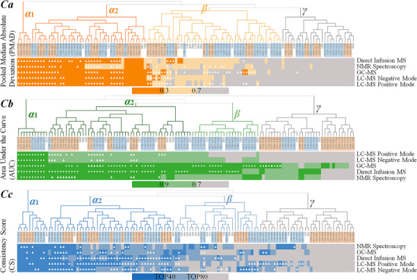
The relationship among the performances of all studied normalization strategies identified based on the hierarchical clustering of the quantitative metrics across all five benchmarks representing different analytical platforms. The analyzed metrics for each criterion (Ca, Cb and Cc) were PMAD, AUC and CS, respectively. The leaves of the hierarchical tree gave the name of the studied strategies. The background colors of the strategies of a single method, sequential combination of ‘sample’-based and ‘metabolite’-based methods and sequential integration of ‘metabolite’-based and ‘sample’-based ones were white, light blue and light orange, respectively. (Ca) The methods with PMAD of superior (≤0.3), good (>0.3 and <0.7) and poor (>0.7) performance were colored by dark orange, light orange and gray, respectively. (Cb) The methods with AUC value of superior (>0.9), good (>0.7 and ≤0.9) and poor (≤0.7) performances were colored by dark green, light green and gray, respectively. If the AUC values of a combined strategy and any single method in this combination equaled to 1 (perfect classification), a white round dot was applied to highlight that strategy. (Cc) The methods that ranked to be the top one-third, bottom one-third and remaining one-third by their CS values were indicated by dark blue, gray and light blue color, respectively. If the performance of a combined strategy was better than both single methods within this combination, a triangle was used to highlight that strategy.

For the criterion Ca, the hierarchical clustering identified four partitions (α1, α2, β and γ, as illustrated in Figure 1Ca and Supplementary Figure S1). The leaves of the hierarchical tree provided the name of the studied strategies. The backgrounds of the strategies of a single method, sequential combination of ‘sample’-based and ‘metabolite’-based methods and sequential combination of ‘metabolite’-based and ‘sample’-based methods were colored in white, light blue and light orange, respectively. The methods with the PMAD of superior (≤0.3), good (>0.3 and <0.7) and poor (>0.7) performance were colored by dark orange, light orange and gray, respectively. If the performance of a combined strategy was better than both single methods in this combination, a triangle was used to highlight that strategy. As shown in Figure 1Ca, the strategies in both Partitions α1 and α2 were discovered to be the ‘consistently well-performing’ (CWP) strategies across all five benchmarks. Particularly, all PMADs in Partition α1 were <0.3, and the majority of the PMADs in Partition α2 were <0.3 with the remaining PMADs within the range between 0.3 and 0.7. The strategies in Partition β were identified as the ‘WP’ ones, since most of the PMADs were within the range between 0.3 and 0.7. The strategies in Partition γ were found to be ‘poor-performing’ with almost all PMADs >0.7. Moreover, most of the ‘triangles’ were concentrated in Partition α, many were in Partition β and very few were in Partition γ.

Similar to Figure 1Ca, the corresponding hierarchical trees (Figure 1Cb and Figure 1Cc) were drawn for criterion Cb and Cc, respectively. The methods with the AUC value of superior (>0.9), good (>0.7 and ≤0.9) and poor (≤0.7) performances were colored by dark green, light green and gray, respectively. If the AUC values of a combined strategy and any single method within this combination equaled to 1.0 (perfect classification), a white round dot was applied to highlight that strategy (Figure 1Cb). The methods that ranked to be the top one-third, the bottom one-third and the remaining one-third by their CS values were indicated by dark blue, gray and light blue color, respectively (Figure 1Cc). Detailed illustrations were also provided in Supplementary Figures S2 and S3. As illustrated, the strategies in both Partitions α1 and α2 were discovered to be ‘CWP’ across all benchmarks, the strategies in Partition β were identified to be ‘WP’ and the strategies in Partition γ were found to be ‘poor-performing’. Moreover, the majority of the ‘triangles’ and ‘round dots’ were concentrated in Partition α, many were in Partition β and very few were in Partition γ.

The strategies identified to be ‘CWP’ or ‘WP’ by each criterion provided valuable information for the discovery of WP strategy. However, due to the distinct underlying theories of the three criteria, the strategies identified by different criteria varied greatly. Thus, the assessments that collectively considered multiple criteria were required.

Performance of the strategies of single method assessed by multiple criteria

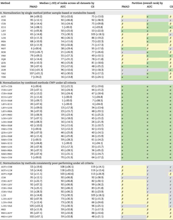
The collective assessment of the performance of the strategies of single method using multiple criteria could be achieved by analyzing the ranks and partitions in Figure 1. Therefore, the quantitative data of the ranks and partitions of each strategy of single method under multiple criteria were provided in Table 3A. On one hand, the ranks of these strategies assessed by a given criterion varied significantly. For example, under criterion Cc, the EigenMS was ranked the 4th (the highest among all strategies of single method), while the Linear Baseline was ranked the 103rd (the lowest among all these strategies). On the other hand, the ranks and partitions of given strategy evaluated by different criteria also varied substantially. For instance, the ranks of MSTUS strategy assessed by PMAD, AUC and CS were 6th (top 5%), 38th (top 32%) and 95th (top 79%), respectively, and its partitions were therefore extensively ranging from α to β to γ. As shown in Figure 2A, none of those 17 methods in Table 1 was partitioned to be CWP under all criteria, and only 5 methods were in Partition α (Figure 1) of two of the three criteria (EIG, LEV, PAR, RAN and VSN). When both Partitions α and β were considered (Figure 2B), 12 single methods were partitioned to be CWP or WP under all criteria. In other words, these popular methods (Table 1) did not provide any normalization strategy capable of performing consistently well irrespective of the studied analytical platform (within Partition α in Figure 1). These results indicated that several methods reported as WP under single criterion (such as VSN [21], QUA [42] and CUB [43]) did not work well under all criteria as identified in this study, and some methods popular in current metabolomics (such as MSTUS [44]) would not perform consistently well under all criteria for all datasets. The detailed partitions of each method could also be found in Table 3A.

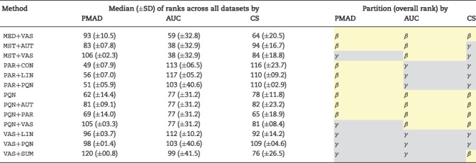
Table 3.

The normalization performance under each criterion (PMAD, AUC and CS) assessed by the ranks of five representative datasets and the clustering partitions (α, β and γ) illustrated in Figure 1. There were three method types: (A) 17 ‘sample/metabolite’-based methods, (B) 21 combined strategies CWP under all three criteria and (C) 28 methods consistently poor-performing under all three criteria. Median and SD represented the median value and the SD of the ranks of five representative datasets, respectively

Figure 2.

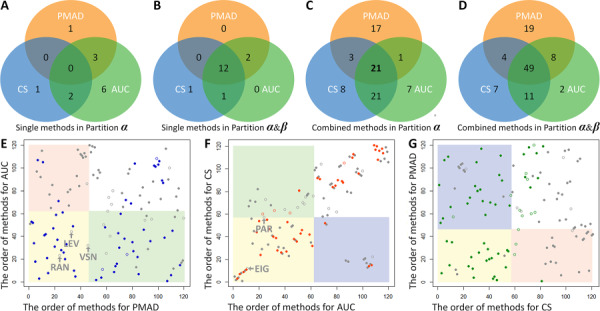
Venn diagram of the numbers of the single method in Partitions α (A) and α&β (B) of Figure 1, and the combined strategy in Partitions α (C) and α&β (D) of Figure 1 by all criteria. Identification of the WP strategy under two of the three criteria based on the orders of the studied strategies ranked by any two criteria in Figure 1. (E) AUC and PMAD; (F) CS and AUC; (G) PMAD and CS.

The incapability of these single methods discussed above might originate from the sole consideration of either ‘sample’-based or ‘metabolite’-based removal of unwanted variation. As the only method based on both ‘sample’ and ‘metabolite’ [45], the VSN was identified to be CWP as assessed by criteria Ca and Cb, and be WP by criterion Cc. Based on the ranks of VSN and other methods in Table 3A, it seemed that VSN was one of the best performing methods in Table 1. This result was consistent with previous report that the VSN performed well in variation reduction and differential expression analysis [9, 21]. Particularly, VSN aimed at keeping the variance constant over the entire data range. ‘First’, the sample-to-sample variations were reduced by linearly mapping the concentration of each sample to a reference sample (the first one in dataset). ‘Then’, the variance was adjusted based on an inverse hyperbolic sine transformation [25, 46]. Due to its hybrid between ‘sample’-based and ‘metabolite’-based normalization, it performed relatively well in adjusting the variance of different samples and metabolites.

Discovering the normalization strategies WP under all criteria

Contrary to the incapability of single methods, the combined strategies showed significantly enhanced performances under all criteria. As shown in Figure 2C, 21 combined strategies were partitioned to be CWP under all three criteria, and another 25 strategies were in Partition α (Figure 1) of two of those three criteria. When both Partitions α and β were considered (Figure 2D), 49 combined strategies were partitioned to be CWP or WP under all criteria, and another 23 strategies were in Partition α (Figure 1) of two of the three criteria. In other words, 21 combined strategies were successfully identified as performing consistently well irrespective of the studied analytical platforms (Partition α in Figure 1). The ranks and partitions of these 21 combined strategies were shown in Table 3B. Moreover, the orders of the studied strategies ranked by any two criteria in Figure 1 were used to draw Figure 2E–G. The round dots and annuluses denoted the combined strategies and single methods, respectively. Those five single methods clustered in Partition α of two of the three criteria (Figure 2A) were marked in Figure 2E and F. Those dots colored in blue (Figure 2E), orange (Figure 2F) and green (Figure 2G) referred to the strategies clustered in Partition α of CS, PMAD and AUC, respectively.

The corresponding assessment values of each of those 21 newly identified strategies were illustrated in Figure 3A and Table 3B. As shown, 11 out of those 17 single methods appeared in these combined strategies for at least one time, which included 6 ‘sample’-based (CUB, LOE, EIG, MEA, QUA, MED) and all 5 ‘metabolite’-based (RAN, LEV, VAS, PAR, AUT) methods. For ‘sample’-based method, CUB appeared the most (in 6 combined strategies), and RAN appeared the most (in 10 combined strategies) among all ‘metabolite’-based methods. To eliminate unbalance between the numbers of ‘sample’-based and ‘metabolite’-based methods, the percentages of each method’s appearance over the total number of its all possible combinations were provided in Figure 3B. As illustrated, the bars colored in light blue and light orange indicated the sequential combination of ‘sample’-based and ‘metabolite’-based methods and sequential combination of ‘metabolite’-based and ‘sample’-based methods, respectively. Six single methods in Table 1 (CUB, RAN, LEV, EIG, LOE and MEA) were found to generate CWP strategies regardless of their position in the corresponding strategy, but different percentages for different positions were observed in Figure 3B. Taking CUB as an example, 80% of the ‘metabolite’-based methods could be followed by CUB to generate CWP strategies, while the percentage reduced to 40% when applying CUB before any ‘metabolite’-based method (Figure 3B). Besides those six single methods, VAS, AUT and PAR were found to generate CWP strategies only by following with ‘sample’-based method, while QUA was discovered to generate CWP strategies by following with ‘metabolite’-based method. MED was also found to form CWP strategies, but only after the application of the ‘metabolite’-based method. A few method combinations had been reported in metabolomic analyses. For example, PAR was used along with MED for analyzing the MS-based metabolomic data [23], QUA and CUB were combined with some ‘metabolite’-based methods to achieve consistent and reproducible results [26] and ‘metabolite’-based methods were used after sample-wised ones before metabolic marker identification [47]. These previous reports further confirmed the usefulness of the novel approach proposed here for identifying the CWP normalization strategy for current metabolomics.

Figure 3.

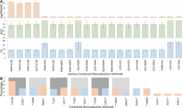
The performances of the 21 newly identified CWP strategies. (A) Quantitative illustrations of the assessing results using PMAD (light orange bar), AUC (light green bar) and CS (light blue bar). (B) The percentages of each method’s appearance over the total number of its possible combinations. The bars colored in light blue and light orange indicated the sequential combination of ‘sample’-based and ‘metabolite’-based methods and the sequential combination of ‘metabolite’-based and ‘sample’-based methods, respectively.

Moreover, 28 strategies were found to be non-CWP under three criteria (none of these strategies was clustered into Partition α of any criterion in Figure 1). The assessment values of each of those 28 ‘badly performing’ strategies were shown in Figure 4A and Table 3C. As shown, 10 out of those 17 single methods appeared in these combined strategies for at least one time, which included 6 ‘sample’-based (PQN, LIN, CON, MED, MST, SUM) and 4 ‘metabolite’-based (VAS, AUT, PAR, LEV) methods. For ‘sample’-based method, PQN, LIN and CON appeared the most (all in six combined strategies), and VAS and AUT appeared the most (both in eight combined strategies) among all ‘metabolite’-based methods. As shown in Figure 4B, six single methods in Table 1 (CON, LIN, PQN, VAS, AUT and PAR) were found to generate ‘badly performing’ strategies regardless of their position in corresponding strategies, but slightly different percentages for different positions were also observed. Taking VAS as an example, 45.5% of ‘sample’-based methods could be followed by VAS to generate ‘badly performing’ strategies, while the percentage reduced to 33.3% when applying VAS before any ‘sample’-based method (Figure 4B). Besides those six methods, MED and MST were found to result in ‘badly performing’ strategies only by following with ‘metabolite’-based method, while LEV was found to lead to ‘badly performing’ strategies by following with ‘sample’-based method. SUM was also found to form ‘badly performing’ strategies, but only after the application of ‘metabolite’-based method. The blue dash line in Figure 4B indicated that four single methods (CON, LIN, MED, PQN) also perform bad under all criteria.

Figure 4.

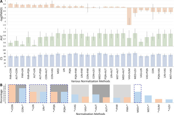
The performances of the 28 ‘badly performing’ strategies. (A) Quantitative illustrations of the assessing results by PMAD (light orange bar), AUC (light green bar) and CS (light blue bar). (B) The percentages of each method’s appearance over the total number of its possible combinations. The bars colored in light blue and light orange indicated the sequential combination of ‘sample’-based and ‘metabolite’-based method and sequential combination of ‘metabolite’-based and ‘sample’-based method, respectively. The blue dash line indicated the single methods performing badly under all criteria.

Conclusion

Herein, various normalization methods (such as CUB, RAN, LEV, EIG, LOE and MEA) were found performing consistently well under all three criteria through combining with other methods other than their normalization type (‘sample’-based or ‘metabolite’-based). Moreover, several other methods (such as CON, LIN, PQN, VAS, AUT and PAR) were discovered to perform badly as assessed by different criteria if they combined with certain methods. However, the dataset-dependent nature was frequently reported in current metabolomic studies [1, 10]. Thus, it was very important to understand the nature of the studied problem in the first place, and then select the appropriate strategies based on the similar pipeline adopted in this study.

 

Qingxia Yang, Jiajun Hong and Yi Li are PhD candidates of Zhejiang University. Their main research interests include OMICs-based bioinformatics and statistical metabolomics.

 

Weiwei Xue is an associate professor of Chongqing University. His main research interests include OMICs, metabolomics and computer-aided drug design.

 

Song Li and Hui Yang are professors of Army Medical University. Their main research interests include the metabolomics-facilitated discovery of anti-cancer therapy for pituitary adenomas.

 

Feng Zhu is a professor of College of Pharmaceutical Sciences in Zhejiang University, China. He got his PhD degree from National University of Singapore. His research group (https://idrblab.org/) has been working in the fields of bioinformatics, OMIC-based drug discovery, system biology and medicinal chemistry. Readers are welcome to visit his personal website at https://idrblab.org/Peoples.php.

 

Key Points

• The discovery of the appropriate normalization methods that can meet multiple criteria in current metabolomics is extremely challenging.

• A novel approach was proposed here to discover the normalization strategies that are CWP under all criteria.

• Twenty-one strategies that combined the ‘sample’-based method with the ‘metabolite’-based one were discovered in this study to be CWP.

• A variety of currently available methods (such as cubic splines and EigenMS) were found to be able to become CWP when combining with other normalization.

Funding

National Key Research and Development Program of China (2018YFC0910500), National Natural Science Foundation of China (81872798), Fundamental Research Fund for Central University (2018QNA7023, 10611CDJXZ238826, 2018CDQYSG0007 and CDJZR14468801) and Innovation Project on Industrial Generic Key Technologies of Chongqing (cstc2015zdcy-ztzx120003). Foundation of Xinqiao Hospital (No.2016YXKJC06).

References

- 1. Li B, Tang J, Yang Q, et al. NOREVA: normalization and evaluation of MS-based metabolomics data. Nucleic Acids Res 2017;45:W162–70. [DOI] [PMC free article] [PubMed] [Google Scholar]
- 2. Chen J, Zhang P, Lv M, et al. Influences of normalization method on biomarker discovery in gas chromatography-mass spectrometry-based untargeted metabolomics: what should be considered? Anal Chem 2017;89:5342–8. [DOI] [PubMed] [Google Scholar]
- 3. De Livera AM, Sysi-Aho M, Jacob L, et al. Statistical methods for handling unwanted variation in metabolomics data. Anal Chem 2015;87:3606–15. [DOI] [PMC free article] [PubMed] [Google Scholar]
- 4. Boysen AK, Heal KR, Carlson LT, et al. Best-matched internal standard normalization in liquid chromatography–mass spectrometry metabolomics applied to environmental samples. Anal Chem 2018;90:1363–9. [DOI] [PubMed] [Google Scholar]
- 5. De Livera AM, Dias DA, De Souza D, et al. Normalizing and integrating metabolomics data. Anal Chem 2012;84:10768–76. [DOI] [PubMed] [Google Scholar]
- 6. Puhka M, Takatalo M, Nordberg ME, et al. Metabolomic profiling of extracellular vesicles and alternative normalization methods reveal enriched metabolites and strategies to study prostate cancer-related changes. Theranostics 2017;7:3824–41. [DOI] [PMC free article] [PubMed] [Google Scholar]
- 7. Gil AM, Duarte D, Pinto J, et al. Assessing exposome effects on pregnancy through urine metabolomics of a Portuguese (Estarreja) cohort. J Proteome Res 2018;17:1278–89. [DOI] [PubMed] [Google Scholar]
- 8. Grams ME, Shafi T, Rhee EP. Metabolomics research in chronic kidney disease. J Am Soc Nephrol 2018;29:1588–90. [DOI] [PMC free article] [PubMed] [Google Scholar]
- 9. Valikangas T, Suomi T, Elo LL. A systematic evaluation of normalization methods in quantitative label-free proteomics. Brief Bioinform 2018;19:1–11. [DOI] [PMC free article] [PubMed] [Google Scholar]
- 10. Chawade A, Alexandersson E, Levander F. Normalyzer: a tool for rapid evaluation of normalization methods for omics data sets. J Proteome Res 2014;13:3114–20. [DOI] [PMC free article] [PubMed] [Google Scholar]
- 11. Wang X, Gardiner EJ, Cairns MJ. Optimal consistency in microRNA expression analysis using reference-gene-based normalization. Mol Biosyst 2015;11:1235–40. [DOI] [PubMed] [Google Scholar]
- 12. Risso D, Ngai J, Speed TP, et al. Normalization of RNA-seq data using factor analysis of control genes or samples. Nat Biotechnol 2014;32:896–902. [DOI] [PMC free article] [PubMed] [Google Scholar]
- 13. Gromski PS, Xu Y, Hollywood KA, et al. The influence of scaling metabolomics data on model classification accuracy. Metabolomics 2015;11:684–95. [Google Scholar]
- 14. Yang Q, Li B, Tang J, et al. Consistent gene signature of schizophrenia identified by a novel feature selection strategy from comprehensive sets of transcriptomic data. Brief Bioinform 2019; doi: 10.1093/bib/bbz049. [DOI] [PubMed] [Google Scholar]
- 15. Li Y, Li X, Hong J, et al. Clinical trials, progression-speed differentiating features and swiftness rule of the innovative targets of first-in-class drugs. Brief Bioinform 2019; doi: 10.1093/bib/bby130. [DOI] [PMC free article] [PubMed] [Google Scholar]
- 16. De Livera AM, Olshansky G, Simpson JA, et al. NormalizeMets: assessing, selecting and implementing statistical methods for normalizing metabolomics data. Metabolomics 2018;14:54. [DOI] [PubMed] [Google Scholar]
- 17. Xia JG, Wishart DS. Web-based inference of biological patterns, functions and pathways from metabolomic data using MetaboAnalyst. Nat Protoc 2011;6:743–60. [DOI] [PubMed] [Google Scholar]
- 18. Willforss J, Chawade A, Levander F. NormalyzerDE: online tool for improved normalization of omics expression data and high-sensitivity differential expression analysis. J Proteome Res 2019;18:732–40. [DOI] [PubMed] [Google Scholar]
- 19. Li XK, Lu QB, Chen WW, et al. Arginine deficiency is involved in thrombocytopenia and immunosuppression in severe fever with thrombocytopenia syndrome. Sci Transl Med 2018;10:eaat4162. [DOI] [PubMed] [Google Scholar]
- 20. Naz S, Kolmert J, Yang M, et al. Metabolomics analysis identifies sex-associated metabotypes of oxidative stress and the autotaxin–lysoPA axis in COPD. Eur Respir J 2017;49:1602322. [DOI] [PMC free article] [PubMed] [Google Scholar]
- 21. Li B, Tang J, Yang Q, et al. Performance evaluation and online realization of data-driven normalization methods used in LC/MS based untargeted metabolomics analysis. Sci Rep 2016;6:38881. [DOI] [PMC free article] [PubMed] [Google Scholar]
- 22. Yin J, Sun W, Li F, et al. VARIDT 1.0: variability of drug transporter database. Nucleic Acids Res 2019; doi: 10.1093/nar/gkz779. [DOI] [PMC free article] [PubMed] [Google Scholar]
- 23. Wang Y, Feng R, He C, et al. An integrated strategy to improve data acquisition and metabolite identification by time-staggered ion lists in UHPLC/Q-TOF MS-based metabolomics. J Pharm Biomed Anal 2018;157:171–9. [DOI] [PubMed] [Google Scholar]
- 24. Gao X, Sanderson SM, Dai Z, et al. Dietary methionine influences therapy in mouse cancer models and alters human metabolism. Nature 2019;572:397–401. [DOI] [PMC free article] [PubMed] [Google Scholar]
- 25. Hochrein J, Zacharias HU, Taruttis F, et al. Data normalization of (1)H NMR metabolite fingerprinting data sets in the presence of unbalanced metabolite regulation. J Proteome Res 2015;14:3217–28. [DOI] [PubMed] [Google Scholar]
- 26. Emwas AH, Saccenti E, Gao X, et al. Recommended strategies for spectral processing and post-processing of 1D (1)H-NMR data of biofluids with a particular focus on urine. Metabolomics 2018;14:31. [DOI] [PMC free article] [PubMed] [Google Scholar]
- 27. Ressom HW, Xiao JF, Tuli L, et al. Utilization of metabolomics to identify serum biomarkers for hepatocellular carcinoma in patients with liver cirrhosis. Anal Chim Acta 2012;743:90–100. [DOI] [PMC free article] [PubMed] [Google Scholar]
- 28. Determan CE, Lusczek ER, Witowski NE, et al. Carbohydrate fed state alters the metabolomic response to hemorrhagic shock and resuscitation in liver. Metabolomics 2014;10:950–7. [Google Scholar]
- 29. Kirwan JA, Weber RJ, Broadhurst DI, et al. Direct infusion mass spectrometry metabolomics dataset: a benchmark for data processing and quality control. Sci Data 2014;1:140012. [DOI] [PMC free article] [PubMed] [Google Scholar]
- 30. Haug K, Salek RM, Conesa P, et al. MetaboLights—an open-access general-purpose repository for metabolomics studies and associated meta-data. Nucleic Acids Res 2013;41:D781–6. [DOI] [PMC free article] [PubMed] [Google Scholar]
- 31. Redestig H, Fukushima A, Stenlund H, et al. Compensation for systematic cross-contribution improves normalization of mass spectrometry based metabolomics data. Anal Chem 2009;81:7974–80. [DOI] [PubMed] [Google Scholar]
- 32. Zhang Y, Ying JB, Hong JJ, et al. How does chirality determine the selective inhibition of histone deacetylase 6? A lesson from Trichostatin A enantiomers based on molecular dynamics. ACS Chem Nerosci 2019;10:2467–80. [DOI] [PubMed] [Google Scholar]
- 33. Kim J, Mouw KW, Polak P, et al. Somatic ERCC2 mutations are associated with a distinct genomic signature in urothelial tumors. Nat Genet 2016;48:600–6. [DOI] [PMC free article] [PubMed] [Google Scholar]
- 34. Letunic I, Bork P. Interactive Tree Of Life (iTOL) v4: recent updates and new developments. Nucleic Acids Res 2019;47:W256–9. [DOI] [PMC free article] [PubMed] [Google Scholar]
- 35. Fu J, Tang J, Wang Y, et al. Discovery of the consistently well-performed analysis chain for SWATH-MS based pharmacoproteomic quantification. Front Pharmacol 2018;9:681. [DOI] [PMC free article] [PubMed] [Google Scholar]
- 36. Jiang J, Yin XY, Song XW, et al. EgoNet identifies differential ego-modules and pathways related to prednisolone resistance in childhood acute lymphoblastic leukemia. Hematology 2018;23:221–7. [DOI] [PubMed] [Google Scholar]
- 37. Tang J, Fu J, Wang Y, et al. Simultaneous improvement in the precision, accuracy, and robustness of label-free proteome quantification by optimizing data manipulation chains. Mol Cell Proteomics 2019;18:1683–99. [DOI] [PMC free article] [PubMed] [Google Scholar]
- 38. Pergoli L, Cantone L, Favero C, et al. Extracellular vesicle-packaged miRNA release after short-term exposure to particulate matter is associated with increased coagulation. Part Fibre Toxicol 2017;14:32. [DOI] [PMC free article] [PubMed] [Google Scholar]
- 39. Oh HK, Tan AL, Das K, et al. Genomic loss of miR-486 regulates tumor progression and the OLFM4 antiapoptotic factor in gastric cancer. Clin Cancer Res 2011;17:2657–67. [DOI] [PubMed] [Google Scholar]
- 40. Tang J, Fu J, Wang Y, et al. ANPELA: analysis and performance assessment of the label-free quantification workflow for metaproteomic studies. Brief Bioinform 2019; doi: 10.1093/bib/bby127. [DOI] [PMC free article] [PubMed] [Google Scholar]
- 41. Xue W, Yang F, Wang P, et al. What contributes to serotonin–norepinephrine reuptake inhibitors' dual-targeting mechanism? The key role of transmembrane domain 6 in human serotonin and norepinephrine transporters revealed by molecular dynamics simulation. ACS Chem Nerosci 2018;9:1128–40. [DOI] [PubMed] [Google Scholar]
- 42. Kohl SM, Klein MS, Hochrein J, et al. State-of-the art data normalization methods improve NMR-based metabolomic analysis. Metabolomics 2012;8:146–60. [DOI] [PMC free article] [PubMed] [Google Scholar]
- 43. Ejigu BA, Valkenborg D, Baggerman G, et al. Evaluation of normalization methods to pave the way towards large-scale LC–MS-based metabolomics profiling experiments. OMICS 2013;17:473–85. [DOI] [PMC free article] [PubMed] [Google Scholar]
- 44. Gagnebin Y, Tonoli D, Lescuyer P, et al. Metabolomic analysis of urine samples by UHPLC-QTOF-MS: impact of normalization strategies. Anal Chim Acta 2017;955:27–35. [DOI] [PubMed] [Google Scholar]
- 45. Saccenti E. Correlation patterns in experimental data are affected by normalization procedures: consequences for data analysis and network inference. J Proteome Res 2017;16:619–34. [DOI] [PubMed] [Google Scholar]
- 46. Huber W, von Heydebreck A, Sultmann H, et al. Variance stabilization applied to microarray data calibration and to the quantification of differential expression. Bioinformatics 2002;18:S96–104. [DOI] [PubMed] [Google Scholar]
- 47. Shen X, Zhu ZJ. MetFlow: an interactive and integrated workflow for metabolomics data cleaning and differential metabolite discovery. Bioinformatics 2019;35:2870–2. [DOI] [PubMed] [Google Scholar]
- 48. Astrand M. Contrast normalization of oligonucleotide arrays. J Comput Biol 2003;10:95–102. [DOI] [PubMed] [Google Scholar]
- 49. Karpievitch YV, Nikolic SB, Wilson R, et al. Metabolomics data normalization with EigenMS. PLoS One 2014;9:e116221. [DOI] [PMC free article] [PubMed] [Google Scholar]
- 50. Karpievitch YV, Taverner T, Adkins JN, et al. Normalization of peak intensities in bottom-up MS-based proteomics using singular value decomposition. Bioinformatics 2009;25:2573–80. [DOI] [PMC free article] [PubMed] [Google Scholar]
- 51. Andjelkovic V, Thompson R. Changes in gene expression in maize kernel in response to water and salt stress. Plant Cell Rep 2006;25:71–9. [DOI] [PubMed] [Google Scholar]
- 52. De Livera AM, Olshansky M, Speed TP. Statistical analysis of metabolomics data. Methods Mol Biol 2013;1055:291–307. [DOI] [PubMed] [Google Scholar]
- 53. Warrack BM, Hnatyshyn S, Ott KH, et al. Normalization strategies for metabonomic analysis of urine samples. J Chromatogr B Analyt Technol Biomed Life Sci 2009;877:547–52. [DOI] [PubMed] [Google Scholar]
- 54. Jacob CC, Dervilly-Pinel G, Biancotto G, et al. Evaluation of specific gravity as normalization strategy for cattle urinary metabolome analysis. Metabolomics 2014;10:627–37. [Google Scholar]
- 55. Dieterle F, Ross A, Schlotterbeck G, et al. Probabilistic quotient normalization as robust method to account for dilution of complex biological mixtures. Application in 1H NMR metabonomics. Anal Chem 2006;78:4281–90. [DOI] [PubMed] [Google Scholar]
- 56. Bolstad BM, Irizarry RA, Astrand M, et al. A comparison of normalization methods for high density oligonucleotide array data based on variance and bias. Bioinformatics 2003;19:185–93. [DOI] [PubMed] [Google Scholar]
- 57. van den Berg RA, Hoefsloot HCJ, Westerhuis JA, et al. Centering, scaling, and transformations: improving the biological information content of metabolomics data. BMC Genomics 2006;7:142. [DOI] [PMC free article] [PubMed] [Google Scholar]
- 58. Smilde AK, van der Werf MJ, Bijlsma S, et al. Fusion of mass spectrometry-based metabolomics data. Anal Chem 2005;77:6729–36. [DOI] [PubMed] [Google Scholar]
Associated Data
This section collects any data citations, data availability statements, or supplementary materials included in this article.