Deep learning based spectral extrapolation for dual-source, dual-energy x-ray computed tomography

Abstract

Purpose:

Data completion is commonly employed in dual-source, dual-energy computed tomography (CT) when physical or hardware constraints limit the field of view (FoV) covered by one of two imaging chains. Practically, dual-energy data completion is accomplished by estimating missing projection data based on the imaging chain with the full FoV and then by appropriately truncating the analytical reconstruction of the data with the smaller FoV. While this approach works well in many clinical applications, there are applications which would benefit from spectral contrast estimates over the larger FoV (spectral extrapolation)—e.g. model-based iterative reconstruction, contrast-enhanced abdominal imaging of large patients, interior tomography, and combined temporal and spectral imaging.

Methods:

To document the fidelity of spectral extrapolation and to prototype a deep learning algorithm to perform it, we assembled a data set of 50 dual-source, dual-energy abdominal x-ray CT scans (acquired at Duke University Medical Center with 5 Siemens Flash scanners; chain A: 50 cm FoV, 100 kV; chain B: 33 cm FoV, 140 kV + Sn; helical pitch: 0.8). Data sets were reconstructed using ReconCT (v14.1, Siemens Healthineers): 768×768 pixels per slice, 50 cm FoV, 0.75 mm slice thickness, “Dual-Energy - WFBP” reconstruction mode with dual-source data completion. A hybrid architecture consisting of a learned piecewise-linear transfer function (PLTF) and a convolutional neural network (CNN) was trained using 40 scans (5 scans reserved for validation, 5 for testing). The PLTF learned to map chain A spectral contrast to chain B spectral contrast voxel-wise, performing an image-domain analog of dual-source data completion with approximate spectral reweighting. The CNN with its U-net structure then learned to improve the accuracy of chain B contrast estimates by copying chain A structural information, by encoding prior chain A, chain B contrast relationships, and by generalizing feature-contrast associations. Training was supervised, using data from within the 33 cm chain B FoV to optimize and assess network performance.

Results:

Extrapolation performance on the testing data confirmed our network’s robustness and ability to generalize to unseen data from different patients, yielding maximum extrapolation errors of 26 HU following the PLTF and 7.5 HU following the CNN (averaged per target organ). Degradation of network performance when applied to a geometrically simple phantom confirmed our method’s reliance on feature-contrast relationships in correctly inferring spectral contrast. Integrating our image-domain spectral extrapolation network into a standard dual-source, dual-energy processing pipeline for Siemens Flash scanner data yielded spectral CT data with adequate fidelity for the generation of both 50 keV monochromatic images and material decomposition images over a 30 cm FoV for chain B when only 20 cm of chain B data was available for spectral extrapolation.

Conclusions:

Even with a moderate amount of training data, deep learning methods are capable of robustly inferring spectral contrast from feature-contrast relationships in spectral CT data, leading to spectral extrapolation performance well beyond what may be expected at face value. Future work reconciling spectral extrapolation results with original projection data is expected to further improve results in outlying and pathological cases.

1. Introduction

In the context of x-ray CT, data completion is the process of extending truncated projection data to avoid artifacts introduced by reconstruction with filtered backprojection. Single-source data completion methods are commonly employed in applications such as the imaging of obese patients to avoid bright banding artifacts at the periphery of the reconstructed field of view (FoV).¹ In this work, we focus on the extension of data completion methods to dual-source, dual-energy CT, where physical or hardware constraints limit the FoV covered by one of two imaging chains.

Perhaps the most well-established application of dual-source data completion is as a preprocessing step for analytical reconstruction of data acquired with Siemens’ dual-source CT scanners (e.g. SOMATOM Definition Flash, SOMATOM Force).² These systems consist of energy-integrating detectors referred to as chain “A,” which covers the scanner’s maximum FoV (here, lower kVp), and chain “B,” which covers a smaller FoV (here, higher kVp). Prior to analytical reconstruction with weighted filtered back projection (WFBP³), the chain B projection data is completed using rescaled chain A data to allow artifact-free projection filtration. In this way, dual-energy imaging and dose-efficient cardiac imaging with high temporal resolution are possible within the FoV of chain B. Recently, Siemens and Mayo Clinic have further expanded these data completion methods for the reconstruction of spectral CT data acquired with their prototype energy-integrating detector (chain A) and photon-counting detector (chain B) hybrid system.⁴ These data completion methods are effective in many practical applications; however, they face several important limitations. For example, virtual non-contrast imaging and material decomposition cannot be performed outside of the FoV of chain B in contrast-enhanced abdominal and chest scans of large patients. Furthermore, in advanced applications such as dual-source, dual-energy cardiac imaging, spectral information is averaged to achieve the highest possible temporal resolution. Finally, in related applications such as model-based reconstruction, interior tomography, and radiation therapy calculations, assumptions are required to handle incompletely sampled data.

Building on earlier work in simulations,⁵ here we propose and demonstrate a refined deep-learning based, image domain approach to spectral extrapolation (formerly referred to as spectral data completion) using clinical CT data. Given dual-source, dual-energy CT data acquired in the configuration described above, spectral extrapolation produces an estimate of chain B spectral contrast over the entire FoV of chain A, with the intent to allow spectral processing over the chain A FoV. At face value, this extrapolation of chain B is ill-conditioned. The attenuation of voxels containing predominantly air, fat, or unenhanced soft tissue may be approximately remapped to chain B attenuation values with a dual-energy histogram, but voxels containing calcium and iodine yield ambiguous attenuation values, with more than one possible material basis describing the contrast relationship between chains. As with all ill-conditioned inverse problems, regularization based on prior information and prior assumptions may be employed to more uniquely determine the problem’s solution.

To this end, we propose a hybrid deep learning method to extrapolate chain B spectral contrast: a learned piecewise linear transfer function (PLTF) and a convolution neural network (CNN). As the name suggests, the PLTF provides an unambiguous mapping of chain A attenuation values (Hounsfield Units, HU) to chain B attenuation values, where the mapped value is determined to provide the minimum mean-squared error over attenuation value pairs seen in the training set. With parallels to data completion for dual-source CT, this chain B image, estimated from chain A, is fused with a seed region from the analytical reconstruction of chain B in the image domain. The chain A and seeded chain B data are passed into a CNN. During training, this multi-resolution CNN, based on the popular U-net architecture,⁶ is expected to encode prior information on both local and non-local feature-contrast relationships relevant to the refinement of the chain B attenuation estimate. In this work, we conduct a series of experiments to demonstrate the feasibility of dual-energy spectral extrapolation and to begin to explore the significance of these forms of prior information to the network’s performance.

While we are the first to demonstrate spectral extrapolation in clinical CT data, we note that there is considerable precedent for the value of deep learning in CT processing pipelines⁷ and the regularization of inverse problems.⁸ This includes a growing body of work on CNN-based post-reconstruction denoising for reproducing full-dose CT data from low-dose CT data.^9–11 More relevant here, this also includes several papers demonstrating the advantages of spatial contextual information in the problems of material decomposition^12–14 and the synthesis of non-contrast images¹⁵ and monochromatic images.¹⁶ More broadly, application of deep learning to the problem of spectral extrapolation is motivated by prior successes in a number of closely related image processing problems, including inpainting,¹⁷ pan-sharpening,¹⁸ and assigning color to grayscale images.¹⁹

2. Materials and Methods

To develop the proposed model for spectral extrapolation, Secs. 2.A and 2.B provide a description of the clinical data used to train, validate, and test the model and the phantom data used to assess the model’s reliance on feature-contrast relationships. Next the model’s construction and training procedures (Sec. 2.C) and experiments used to test the model’s performance (Sec. 2.D) are described. Finally, Sec. 2.E details a plan to incorporate the trained model into current clinical dual-source, dual-energy data processing workflows.

2.A. Clinical data

Training, validation, and testing of the proposed model was conducted with a set of 50 dual-source, dual-energy abdominal x-ray CT scans (acquired with 5 Siemens SOMATOM Flash scanners: 2x Duke Hospital, 1x Duke Emergency Department, 2x Duke Cancer Center; Siemens Healthineers, Forchheim, Germany) and included projection data for each scan. The data was collected retrospectively as part of a research study approved by Duke University Medical Center’s Institutional Review Board (IRB# Pro00102466). The patient population included 21 females and 29 males with the aggregate statistics shown in Table 1. All scans followed a consistent protocol for contrast-enhanced portal venous phase imaging. ISOVUE-370 iodine-based contrast agent (Bracco, Milan, Italy) was injected in 6 patients, while ISOVUE-300 was used for all other patients. The average contrast agent dose was 151.1 mL (± 23.5 SD).

Table 1.

Patient statistics.

	Average	SD	Minimum	Maximum
Height (cm)	170.54	9.63	144.8	188.0
Weight (kg)	79.44	16.43	42.9	112.4
BMI	27.30	5.30	18.5	38.8
Age (years)	60.58	14.31	17	85

The Flash scanners were operated with a consistent imaging protocol: chain A (50 cm FoV) operating at 100 kVp, chain B (33 cm FoV) operating at 140 kVp with a Sn filter, helical pitch of 0.8, and CARE Dose4D enabled. The quality control program for all of these scanners meets or exceeds standards set by the American College of Radiology.²⁰ All reconstructions were performed using research software, which reproduces protocols accessible from the scanner console (ReconCT v14.1; Siemens Healthineers, Erlangen, Germany). Reconstruction parameters included 768×768 pixels per slice, a 50 cm FoV (0.651×0.651 mm in-plane voxel size), 0.75 mm thick slices every 0.75 mm, and the “Dual-Energy - WFBP” reconstruction mode using the D30f reconstruction kernel. Notably, deviation from the standard image matrix size (512×512) allowed consistent reconstruction for the 50 cm FoV of chain A and approximately isotropic image voxels, standardizing the data for network training and testing. Furthermore, the reconstruction protocol produced an estimate of the chain B reconstruction over the entire 50 cm FoV of chain A, reconstructed following projection domain data completion of the chain B projection data with the chain A projection data. This estimated data is for artifact free reconstruction only and is not displayed or further processed in clinical software.

2.B. Phantom data

Two variants of the Gammex Multi-Energy CT Phantom (Middleton, WI)²¹ were scanned to assess the potential influence of beam hardening on network performance and to study network performance in the absence of strong feature-contrast relationships. Data from this phantom was excluded from network training and validation. The phantom data was scanned and reconstructed using Flash scan parameters and ReconCT reconstruction parameters identical to those described for the patient data in Sec. 2.A. The phantom includes a number of interchangeable material rods (~3 cm diameter) inserted in a 20 cm head phantom or a 40×30 cm torso phantom made from water attenuation equivalent plastic (HE CT Solid Water®). Each rod contains a reference material, including adipose, muscle, iodine (2, 5, 10, 15 mg/mL), iodine in blood (2, 4 mg/mL), and calcium (50, 100, 300 mg/mL).

2.C. Network setup and training

The general strategy for training and testing the proposed spectral extrapolation network is outlined in Fig. 1. Because the true reconstruction for chain B outside of 33 cm is not known, a smaller training mask is defined (red, dashed circle) and the halo between this training mask and a 30 cm chain B mask (blue, solid circle) is extrapolated and compared with the known chain B reconstruction (training labels). As described below, the known chain B reconstruction is inserted inside of the training mask during network evaluation to seed the extrapolation of spectral contrast within the halo. To ensure that the halo always includes meaningful image data for patients and anatomy of varying size, the size of the training mask is dynamically adjusted (between 4–24 cm in 2 cm increments) to the smallest diameter which contains at least 35% of the total image intensity (intensity scale: HU/1000 + 1.0; average diameter: 20 cm; adjusted per 2D image slice). Notably, the chain B mask diameter (30 cm) is intentionally set to be slightly smaller than the chain B FoV (33 cm) to accommodate blending of chain A and B projection data which occurs during projection-domain data completion. Overall, this training strategy has several advantages. Due to the spatial invariance of CNNs, this strategy exactly reproduces the problem of extrapolating spectral contrast between the normal chain B FoV and the chain A FoV, allowing the trained network to be applied within standard clinical processing pipelines. Also, seeding the chain B data with the true chain B reconstruction, within the training mask, and then minimizing the training cost over the entire chain B mask (not just the halo) grounds the network to produce unbiased extrapolation results.

Fig. 1.

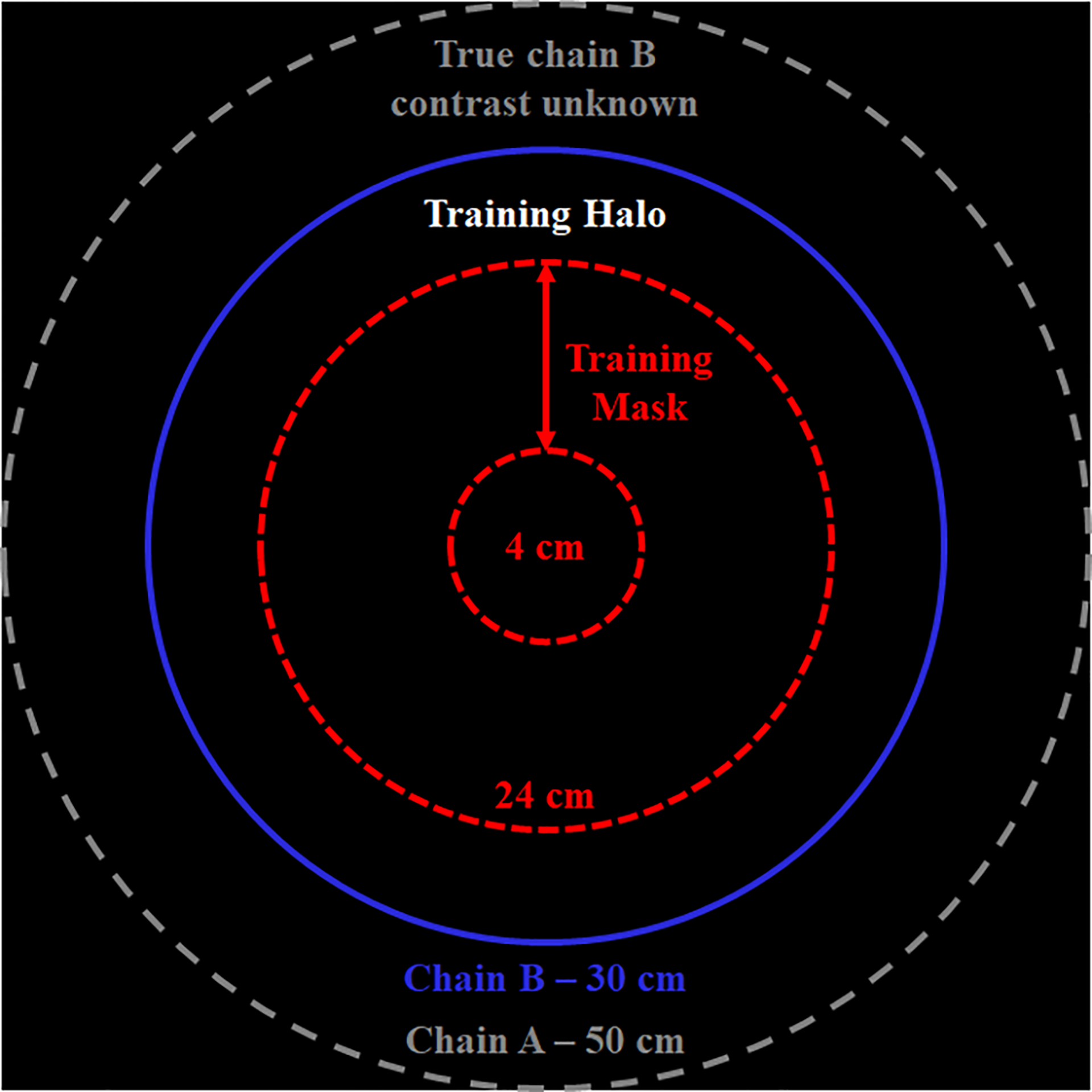
Spectral extrapolation training and testing strategy. Because the true chain B contrast is only known within a restricted FoV (blue solid circle, chain B mask), a smaller training mask is defined (red, dashed circle) and the training halo between the training mask and the chain B mask is extrapolated and compared with the known chain B reconstruction (training labels). To accommodate varying patient sizes and anatomy, the size of the training mask was dynamically adjusted (between 4 and 24 cm; average diameter: 20 cm). Diagram not to scale.

Network training and evaluation proceeds in two steps: (1) the estimation of chain B attenuation by the application of a PLTF to the chain A data and (2) the evaluation of a CNN. The PLTF, shown in Fig. 2, included 17 trainable parameters, learned coefficients (c), and their corresponding fixed grid points (g). The grid points were placed at −2000 HU, 3000 HU, and at 200 HU increments from −1000 to 1800 HU (chain A attenuation values). Given the attenuation of the chain A data, X_A, at voxel n, an estimate of the chain B attenuation, X_AB, is then produced by evaluating the following equation:

$${\text{X}}_{\text{AB}}\left(n\right)=\text{PLTF}\left({\text{X}}_{\text{A}}\left(n\right)\right)=\frac{({\text{X}}_{\text{A}}\left(n\right)-{\text{g}}_{\text{Low}})}{\left({\text{g}}_{\text{High}}-{\text{g}}_{\text{Low}}\right)}{\text{c}}_{\text{High}}+\frac{\left({\text{g}}_{\text{High}}-{\text{X}}_{\text{A}}\left(n\right)\right)}{\left({\text{g}}_{\text{High}}-{\text{g}}_{\text{Low}}\right)}{\text{c}}_{\text{Low}},$$

$${\text{g}}_{\text{Low}}\le {\text{X}}_{\text{A}}\left(n\right)<{\text{g}}_{\text{High}}$$ (1)

Evaluation of this equation amounts to linear interpolation between the learned coefficients (chain B attenuation values) associated with the grid points nearest to the input chain A attenuation value: g_Low, g_High. To ensure fast convergence during training, the coefficient values were initially set to the values of their corresponding grid points (identity mapping: X_AB(n) = X_A(n)). The objective function minimized during network training was root-mean-squared error (RMSE):

$$\text{RMSE}\left({\text{X}}_{\text{AB}},{\text{X}}_{\text{B}}\right)=\sqrt{\frac{1}{{\text{N}}_{\text{B}}}{\sum }_{n\in {\text{mask}}_{\text{B}}}{\left({\text{X}}_{\text{AB}}\left(n\right)-{\text{X}}_{\text{B}}\left(n\right)\right)}^2},$$ (2)

Where N_B denotes the number of voxels in the chain B mask (mask_B) and X_B denotes the known chain B reconstruction. Notably, the PLTF and the CNN (described next) were trained simultaneously for convenience. The PLTF minimized the objective in Eq. 2 only and was not updated with gradients backpropagated from the CNN.

Fig. 2.

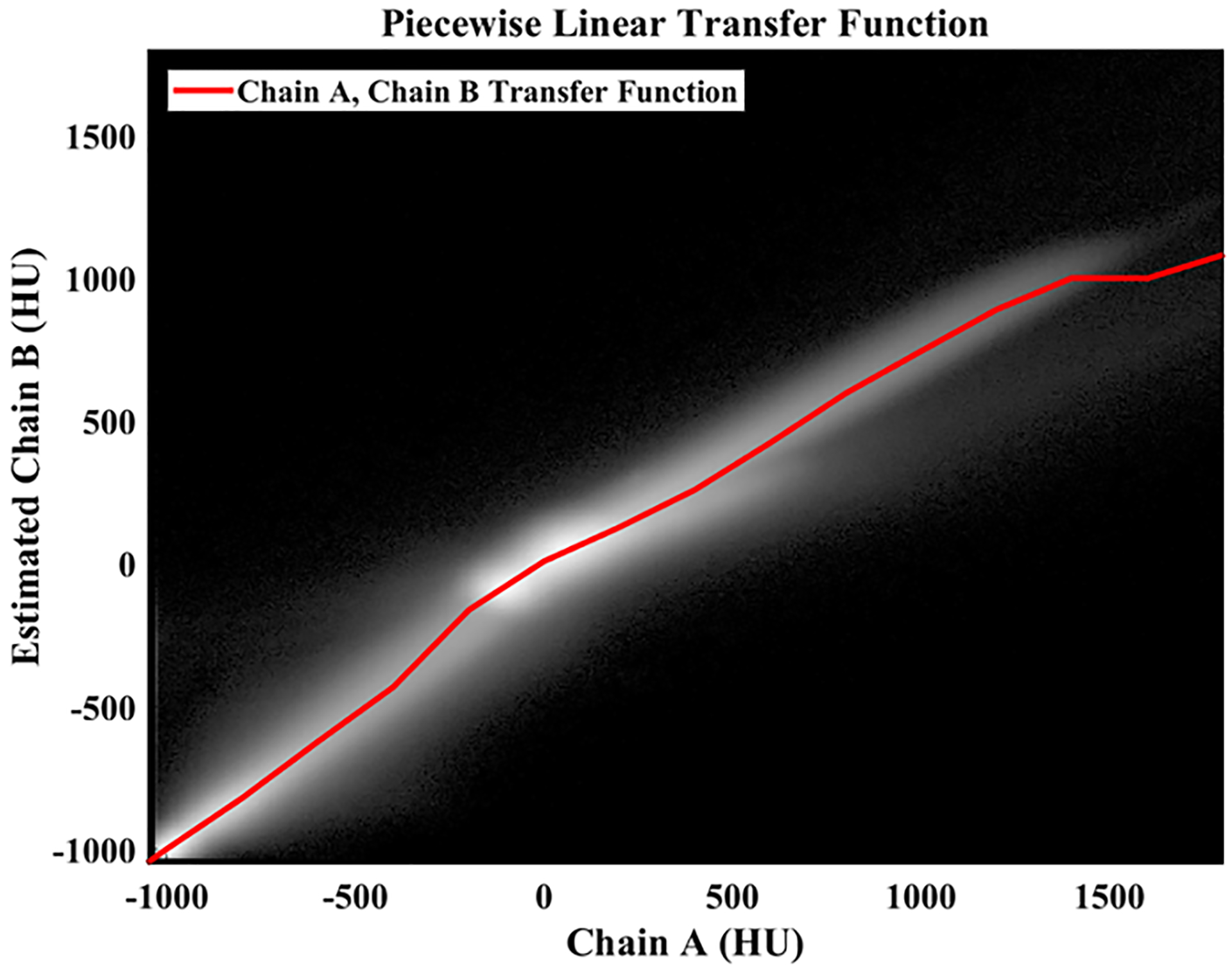
Learned piecewise linear transfer function (PLTF). Background: 2D histogram of chain A and chain B attenuation values measured in Hounsfield units (HU) and computed over the entire training data set (within the FoV of chain B; natural log intensity scale). The learned PLTF is shown as a red line and maps chain A attenuation values (x-axis) to chain B attenuation values (y-axis) to minimize root-mean-squared error.

Prior to evaluation of the CNN, the estimated chain B data, X_AB, is fused with the known chain B reconstruction, X_B (Fig. 3A–B). Specifically, X_AB voxels within the training mask (Fig. 1) are replaced with X_B voxels. This composite image and the original chain A reconstruction, X_A, are then the inputs to the CNN (Fig. 3C; collectively, X₀; bold denotes N_e = 2 total energy channels indexed by e). To couple the chain A and B data during CNN processing and to better zero center the data, a low pass residual connection is employed (Fig. 3D):

$${\text{X}}_{\text{LP}}=\text{G}\otimes \left(\frac{1}{{\text{N}}_e}{\sum }_e{X}_{0,e}\right),$$ (3)

$${\mathbf{\text{X}}}_{\text{HP},e}={\mathbf{\text{X}}}_{0,e}-{\text{X}}_{\text{LP}}.$$ (4)

Low-pass filtration of the energy average is performed by convolution (⨂) with a 2D Gaussian kernel, G, (FWHM, 7 voxels; kernel diameter, 15 voxels) yielding X_LP (Eq. 3). This low-pass, energy average image is then subtracted from each CNN input channel (X_HP, Eq. 4) and added back to each CNN output channel (Fig. 3F; yields Y_A, Y_B). The CNN itself (Fig. 3E) is a 5-level U-net⁶ which uses paired 3×3 convolution kernels with leaky ReLU activation functions²² (no activation after the last convolution layer), 2×2 bilinear up- and down-sampling, skip connections between the input and output branches of the network with feature map concatenation, and padded convolution operations (reflection padding). The depth of the network is calibrated to approximately span the average distance between the training mask (~20 cm) and the chain B mask (30 cm) following two 3×3 convolution operations (average halo size: 5 cm; effective kernel size at level 5: 3.1 cm). Similar to Eq. 2, the CNN was trained to minimize two RMSE objective functions with equal weight:

$$\text{RMSE}\left({\text{X}}_{\text{A}},{\text{Y}}_{\text{A}}\right)=\sqrt{\frac{1}{{\text{N}}_{\text{A}}}{\sum }_n{\left({\text{X}}_{\text{A}}\left(n\right)-{\text{Y}}_{\text{A}}\left(n\right)\right)}^2},$$ (5)

$$\text{RMSE}\left({\text{X}}_{\text{B}},{\text{Y}}_{\text{B}}\right)=\sqrt{\frac{1}{{\text{N}}_{\text{B}}}{\sum }_{n\in {\text{mask}}_{\text{B}}}{\left({\text{X}}_{\text{B}}\left(n\right)-{\text{Y}}_{\text{B}}\left(n\right)\right)}^2}.$$ (6)

Fig. 3.

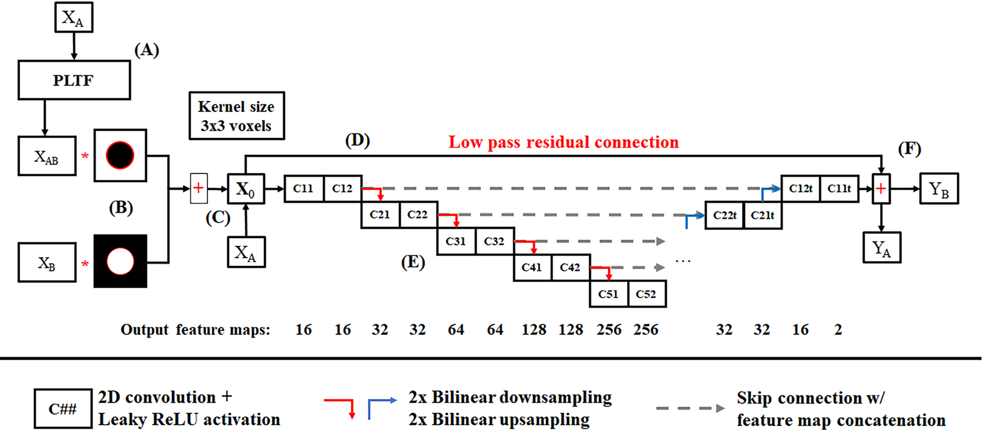
Convolutional neural network (CNN) for spectral extrapolation. (A) X_AB, the output of the PLTF applied to the chain A reconstruction, and X_B, the chain B reconstruction, are fused with a masking procedure (B) (Fig. 1), and the composite image and the original chain A reconstruction, X_A, are passed as two separate channels into the CNN (C). (D) To control intensity bias and to zero center the network inputs, the network inputs are low-pass filtered and the average of the two input channels is subtracted from the network inputs, X₀, and then is added back to the network outputs. (E) The CNN is a U-net which uses bilinear up- and down-sampling, skip connections with feature map concatenation, and a symmetric arrangement of padded convolution operations. (F) The network outputs, Y_A and Y_B, ensure the preservation of chain A contrast and the recovery of chain B contrast, respectively, under a root-mean-squared error penalty function.

Concurrent training of the PLTF and the CNN was conducted using Keras (keras.io), Tensorflow (v.2.0.0; tensorflow.org), and Python (v3.6.8, python.org). Prior to training, the 50 patient data sets, each reconstructed with 0.75 mm slices, were averaged to produce non-overlapping, 3 mm thick slices, yielding a total of ~5000 2D, axial slices (per chain) for training, validation, and testing. The 3 mm slice thickness was chosen because it reflects a common choice in clinical workflows. 40 patient data sets were used for network training, while 5 patient data sets were reserved for network optimization and validation during training (evaluated after every 5^th epoch) and 5 other patient data sets were reserved for testing the final trained network. Training proceeded with a mini-batch size of four 768×768 slices reconstructed for chain A and chain B, with each 2D slice evaluated once per epoch. Data augmentation during training included random assignment of individual slices across patients to mini-batches, random flipping and rotation of the input slices (±180°), and random translation of the training mask within the fixed chain B mask (Fig. 1). Data augmentation was not applied to the validation or testing data. Prior to network evaluation the data for each chain was linearly rescaled from HU to 0 in air and 1 in water, scaling which is reversed after network evaluation. The network’s objective functions were minimized using the ADAM optimizer²³ (β₁, 0.9; β₂, 0.999; learning rate, 3e-4; learning rate decay, 8.8e-5; L2 weight decay, 0.3). Training spanned 100 epochs and was performed with a NVIDIA Quadro RTX 8000 GPU on an Ubuntu 18.04 Linux workstation with 64 GB of RAM and an Intel i7 5960X CPU (total training time: 7.5 hours). Using the same hardware and software, the network can be evaluated on 100 slices (the average number of 3.0 mm slices per patient) in less than 10 seconds.

2.D. Network testing

Prior to network training, a test was conducted with the Gammex phantom to gauge the suitability of a CNN-based solution to the spectral extrapolation problem. Specifically, because CNNs are spatially invariant and consider data within a limited receptive field, it was necessary to confirm the linearity of contrast material measurements (here, calcium, iodine) as a function of non-linear effects such as scatter and beam hardening and their associated corrections applied by Siemens software. If the relationship between contrast materials and their associated HU values does not remain linear as a function of patient size, for instance, then it would be difficult or impossible to train a CNN to correctly extrapolate spectral contrast because it cannot inherently consider patient size. Furthermore, even if the network could compensate for such factors, it would introduce inconsistencies between the extrapolated data and Siemens spectral processing, making the network incompatible with current clinical workflows. To test the linearity of spectral contrast measurements as a function of patient size, the 20 cm Gammex head phantom and the 30×40 cm Gammex torso phantom were imaged with the scanning protocol described in Sec 2.A. The configuration of iodine (2 mg/mL, 5 mg/mL, 15 mg/mL) and calcium (50 mg/mL, 100 mg/mL) inserts remained the same between scans, and linear regression was used to characterize the effects of patient size on spectral contrast.

Following network training, both the validation and testing results were qualitatively and quantitatively assessed. Qualitative evaluation enabled general assessment of network performance in terms of image texture preservation and the identification of outlying cases where the network failed to accurately extrapolate spectral contrast. Quantitative evaluation included the analysis of residual images computed relative to the expected chain B reconstructions and HU error measurements within anatomically relevant regions of interest (ROIs). Overall, the testing data performance was summarized by measuring average contrast recovery errors and their standard deviations as a function of network stage (after the PLTF, after the CNN), patient (5 total), and target organ (liver, right kidney, left kidney, spleen). Organ segmentations were performed semi-automatically using the Avizo software package (v9.3; Thermo Fisher Scientific, Waltham, MA). Error measurements were taken only at the intersection of the training halo (Fig. 1) and the target organs.

The trained network was also applied to the 30×40 cm Gammex torso phantom containing various fat, muscle, blood, iodine, and calcium equivalent inserts to gauge the network’s worst-case performance—i.e. when it is applied to data with no meaningful correlations between image structure and spectral contrast. Network performance was quantitatively measured as a function of location (inside the training mask, inside and beyond the training halo), network stage (after the PLTF, after the CNN), and material. Modulation transfer function (MTF) measurements were also taken as a function of location to assess the impact of spectral extrapolation on spatial resolution. To partially control for the non-linear nature of CNNs, the MTF measurements were derived from radial line profiles drawn through similarly high contrast material rods (15 mg/mL I, 100 mg/mL Ca). These line profiles were used to measure the average edge spread function and then the axial MTF.²⁴

2.E. Deep-learning enhanced dual-source, dual-energy data processing workflow

To demonstrate the network’s potential incorporation into existing clinical workflows for dual-source, dual-energy CT, spectral processing results were compared between a standard clinical workflow and the proposed extrapolation workflow. The standard workflow included the previously described reconstruction with ReconCT followed by the synthesis of 50 keV monochromatic images, quantitative iodine material maps, and virtual non-contrast (VNC) images (3 mm slice thickness) using the syngo.via software package (Siemens Healthineers, Forchheim, Germany). The extrapolation workflow was identical to the standard workflow except that the chain B data was masked and then extrapolated within the training halo prior to spectral processing. The workflows are compared qualitatively, through visual assessment, and quantitatively through signal-to-noise ratio (SNR) measurements and mean iodine concentration measurements (mg/mL) taken within ROIs located in the training halo.

Finally, to demonstrate the uniformity of spectral extrapolation results for performing quantitative spectral measurements, contrast-enhanced liver parenchyma measurements from one of the testing data sets are compared between the training mask (20 cm), the training halo (20–30 cm), and beyond the training halo (30+ cm). The same measurement ROIs are used for comparison across the extrapolated chain B data, the iodine material map, and the VNC image (1 cm slice thickness). Notably, because the syngo.via software package does not perform spectral processing outside of the nominal chain B FoV for Flash scanner data (33 cm), clinically consistent conversion of the iodine map to mg/mL units was not possible. Instead, the iodine and VNC measurements are presented as fractions of contrast measurements taken in the lumen of the abdominal aorta (iodine map: 75 HU; VNC image: 59 HU).

3. Results

3.A. Network training and testing

Fig. 4 numerically summarizes the results of training the PLTF and CNN over 100 epochs for the 40 training data sets (red, solid lines) and the 5 validation data sets (blue, dashed lines). Given only 17 free parameters, the PLTF cost (Fig. 4.1, Eq. 2) converges within the first 10 epochs for both the validation data and the training data without obvious generalization error or overfitting (note the y-axis scale). Visually, the CNN outputs for chain A (Fig. 4.2, Eq. 5) and chain B (Fig. 4.3, Eq. 6) converge after roughly 100 epochs (1.96 million free parameters). The average errors in the chain A output, Y_A, are negligible (below 1 HU) with strong agreement in the CNN’s performance between the training and validation data. The average errors in the chain B output, Y_B, which are measured within the 30 cm chain B training mask, are below 22 HU for both the training and validation data at convergence. There is some variation in the validation data performance with epoch; however, there is a negligible difference in the validation and testing performance overall, ruling out generalization errors and model overfitting.

Fig. 4.

Training (red, solid) and validation (blue, dashed) cost function values by epoch for the proposed network. The validation data sets were evaluated once every 5 epochs. (1) PLTF results evaluated within the 30 cm mask for chain B (Eq. 2). (2) Cost computed for the final network output for chain A, Y_A, over the 50 cm FoV of chain A (Eq. 5). (3) Cost computed for the final network output for chain B, Y_B, within the 30 cm mask for chain B (Eq. 6).

Following network training, Fig. 5 highlights network testing results produced with one of the five testing data sets not seen during network training. Matching ReconCT reconstructions are shown for chain A (1) and chain B (2) in comparison with the network outputs (PLTF and CNN) for chain A (3) and chain B (4) (3 mm slice thickness). Consistent with the training curves reporting negligible output errors for chain A, the chain A network input and output are effectively identical. The chain B input and output are nearly identical within the chain B training mask (see Fig. 5.8); however, image smoothing is observed outside of the training mask. Fig 5.6–5.8 display the attenuation differences between the chain A and chain B network inputs (6) and between the chain B network input and the output of the PLTF (7) and then the CNN (8). These images visualize the success of spectral extrapolation with the expectation of zero difference between the chain B network input and the chain B network output. ROIs (yellow, dashed circles) drawn in fat, contrast-enhanced kidney, and the spleen report mean attenuation values measured in these difference maps. Notably, the 17 parameter PLTF nearly equates the chain A attenuation values to the chain B attenuation values in all three regions; however, correlated differences in attenuation are still visible in regions of high contrast such as the kidneys, the aorta, and the spinal column (Fig. 5.7). Evaluation of the CNN eliminates these remaining differences in the training halo while explicitly preserving the chain B data introduced inside of the red training mask (inner mask, Fig. 5.8).

Fig. 5.

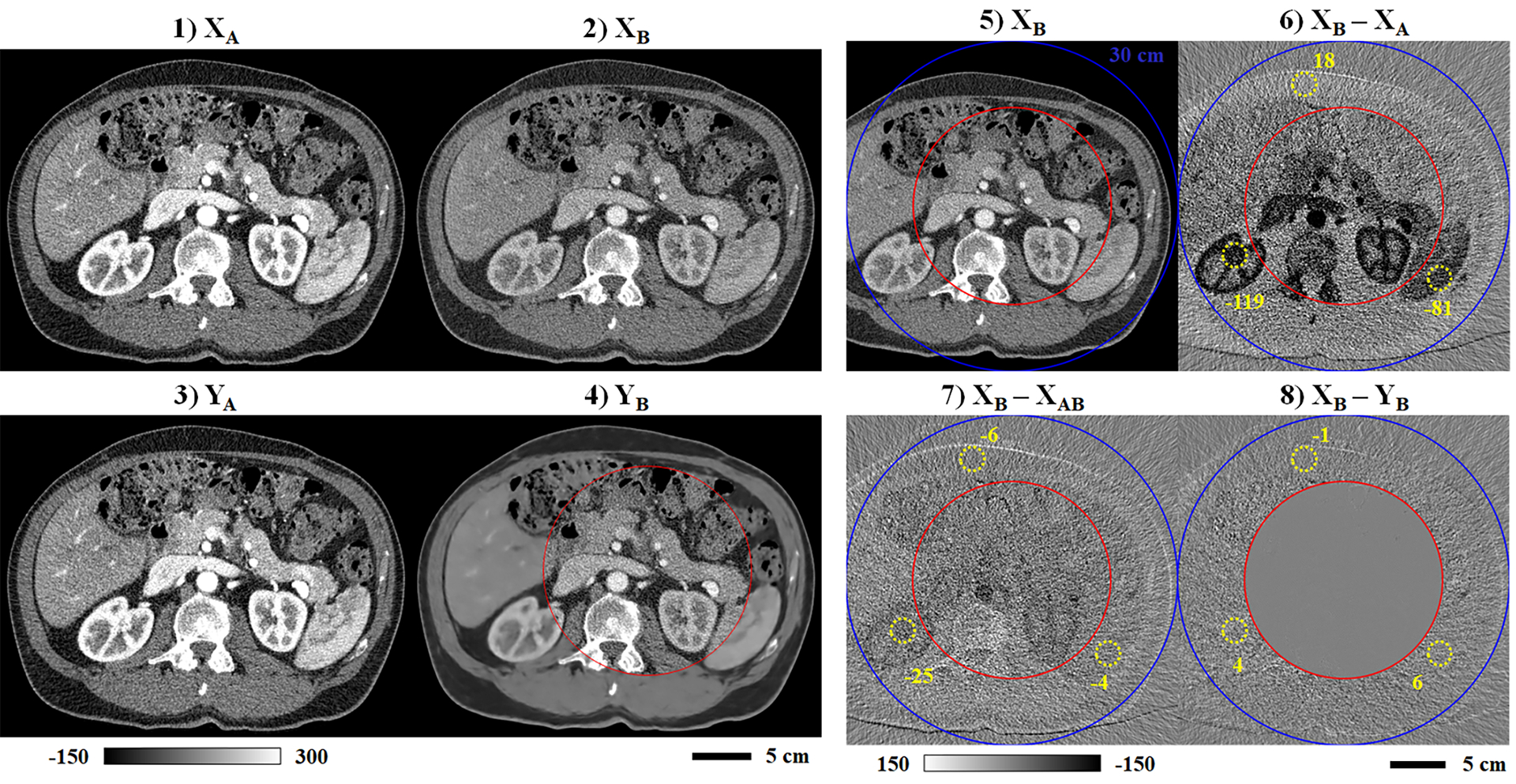
Sample network testing results (3 mm slice thickness). Matching network inputs are shown for chain A (1) and chain B (2). Matching network outputs (PLTF and CNN) are also shown for chain A (3) and chain B (4). (5) Repeat of the chain B input (2), including the 30 cm chain B mask (outer mask, blue) and the training mask (inner mask, red). Intensity differences are shown computed between the original chain B reconstruction and the chain A reconstruction (6), the PLTF estimate of the chain B contrast (7), and the final CNN output for chain B (8). Matching, dashed yellow circles denote regions of interest and the average intensity measured inside (HU). Calibration bar units: HU.

Following the format of Fig. 5, Fig. 6 summarizes the trained network’s performance on one of the validation data sets, highlighting an outlying case where spectral extrapolation fails to accurately recover spectral contrast. As shown in Fig. 6.1–6.2, the ROI (yellow square) includes a cystic lesion in the cortex of the right kidney with higher measured attenuation in the chain B reconstruction (113 HU) than in the chain A reconstruction (107 HU). Because this defect falls within the training halo and is extrapolated based on the chain A data, the extrapolated chain B image structure (Fig. 6.4, inset) closely resembles the chain A data rather than the original chain B data. Furthermore, the extrapolated attenuation, 73 HU, is lower than the chain A attenuation, 107 HU, as would normally be expected. Referencing the difference images (Fig. 6.6–6.8), an extrapolation error of 40 HU in recovering this cystic lesion is clearly visible following evaluation of the PLFT and persists following evaluation of the CNN.

Fig. 6.

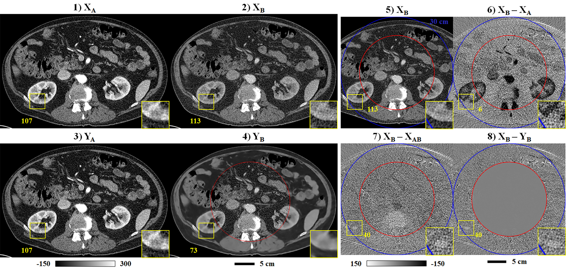
Notable error in spectral extrapolation results (validation data). Following the format of Fig. 5, the network inputs (1–2) and outputs (3–4) are shown for chains A and B (3 mm slice thickness). Yellow squares and corresponding insets (240% zoom) denote the location of an apparent cystic lesion of the kidney cortex with a higher HU value measured in the chain B data than in the chain A data (yellow text). This feature is not correctly recovered following spectral extrapolation (4). (5) Repeat of the chain B input (2), including the 30 cm chain B mask (outer mask, blue) and the training mask (inner mask, red). Calibration bar units: HU.

Finally, Fig. 7 and Table 2 summarize the trained network’s performance on all five test data sets, broken down into mean values measured in target organs: liver, right kidney, left kidney, and spleen. The measurements are restricted to the intersection of each target organ with the training halo to measure the success of spectral extrapolation (see voxel counts in Table 2). Similar to the difference images in Figs. 5–6, the success of spectral extrapolation is measured by comparing the initial difference in attenuation between chains A and B (|X_B – X_A|, blue) with the difference from the known chain B reconstruction after the PLTF (|X_B – X_AB|, red) and then after the CNN (|X_B – Y_B|, yellow). Overall, the PLTF corrects a majority of the attenuation difference between chains A and B, estimating the expected chain B contrast to within 26 HU across all test cases and target organs. With the exception of several small errors in the spleen, the CNN further improves the chain B contrast estimation accuracy for each case and target organ, resulting in maximum average errors below 7.5 HU. Notably, small thumbnail sized images are included with each plot to show the diversity in patient size represented in the testing set. The exact error measurements with their corresponding signs and standard deviations are included in Table 2. This table confirms the reported error measurements and shows that the precision of the spectral extrapolation measurements improves following both the PLTF and the CNN.

Fig. 7.

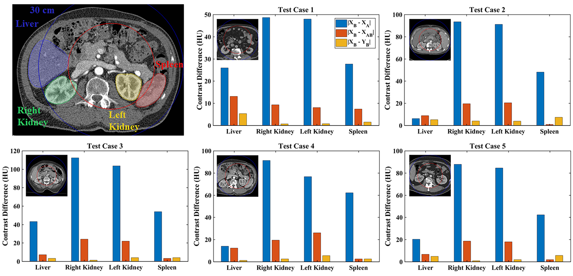
Summary of spectral extrapolation results by segmented organ (colored labels) and test data case (1–5). Mean absolute intensity differences measured in the halo between the chain B mask (outer blue circle) and the training mask (inner red circle) are plotted for each stage of the spectral extrapolation process: network inputs (X_B – X_A), PLTF function output (X_B – X_AB), CNN output (X_B – Y_B). Results are measured over all 3 mm thick slices containing the target anatomy (no overlap between slices). A small thumbnail image is shown for each test case.

Table 2.

Testing results by case and target organ (HU).

Test Case	Organ	Voxel Count (x10,000)	XB - XA		XB - XAB		XB - YB
			Mean	Stdev.	Mean	Stdev.	Mean	Stdev.
1	Liver	49.67	−25.95	56.18	13.13	43.78	5.34	35.01
	Right Kidney	13.71	−48.64	62.83	−9.32	44.59	−0.69	36.61
	Left Kidney	10.59	−47.99	60.88	−8.07	43.25	−0.75	35.48
	Spleen	8.04	−27.69	49.02	7.38	38.97	−1.51	31.62
2	Liver	72.87	−6.24	36.17	8.82	28.87	−5.29	24.16
	Right Kidney	6.41	−93.46	50.48	−19.68	32.92	−4.05	27.19
	Left Kidney	5.18	−91.07	54.73	−20.42	32.88	−3.95	26.73
	Spleen	49.54	−48.05	42.03	−0.94	31.28	−7.43	26.13
3	Liver	38.97	−43.17	34.09	7.15	26.40	3.35	21.97
	Right Kidney	3.99	−112.32	51.81	−24.19	31.21	1.26	25.93
	Left Kidney	4.57	−103.58	56.95	−21.94	31.12	4.05	25.83
	Spleen	4.66	−53.90	34.00	3.23	26.70	4.05	22.49
4	Liver	78.05	−13.99	46.77	12.36	36.36	1.29	29.95
	Right Kidney	13.98	−91.25	69.12	−19.38	42.12	2.49	34.70
	Left Kidney	0.02	−76.78	74.80	−26.12	37.31	5.53	24.07
	Spleen	16.39	−62.25	47.80	−2.52	34.21	2.57	28.45
5	Liver	131.08	−20.33	49.67	6.67	38.88	−4.90	32.28
	Right Kidney	7.44	−87.76	60.45	−18.65	41.20	−0.85	34.03
	Left Kidney	11.76	−84.55	61.69	−18.04	41.11	−1.85	34.29
	Spleen	41.52	−42.29	46.32	1.87	36.02	−5.76	30.12

Note: Bold text indicates the lowest magnitude mean and standard deviation (Stdev.) value in each row.

3.B. Gammex phantom

Fig. 8 shows material sensitivity measurements (3) taken in the Gammex head phantom (1) and torso phantom (2). By measuring the same material rods in each variant of the phantom, changes in apparent calcium (Ca, blue) and iodine (I, red) attenuation as function of phantom size can be visualized. As expected, calcium (50, 100 mg/mL) and iodine (2, 5, 15 mg/mL) attenuation values are underestimated in the torso phantom (‘x’ markers) relative to the head phantom (‘o’ markers) due to beam hardening, particularly at the highest concentration of each material. Despite this effect, linear regression through each set of measurements quantifies the strong linearity of attenuation measured in these reference materials with concentration (Pearson correlation coefficients > 0.99). These results demonstrate that even in the presence of modest beam hardening, it is reasonable to expect a spatially invariant CNN to be able to perform spectral extrapolation because beam hardening manifests as an apparent change in concentration rather than as apparent change in material composition. Furthermore, it is expected that any beam hardening compensations applied during material decomposition in clinical software will apply equally well to extrapolated data because extrapolation will recover the apparent concentration without corrections.

Fig. 8.

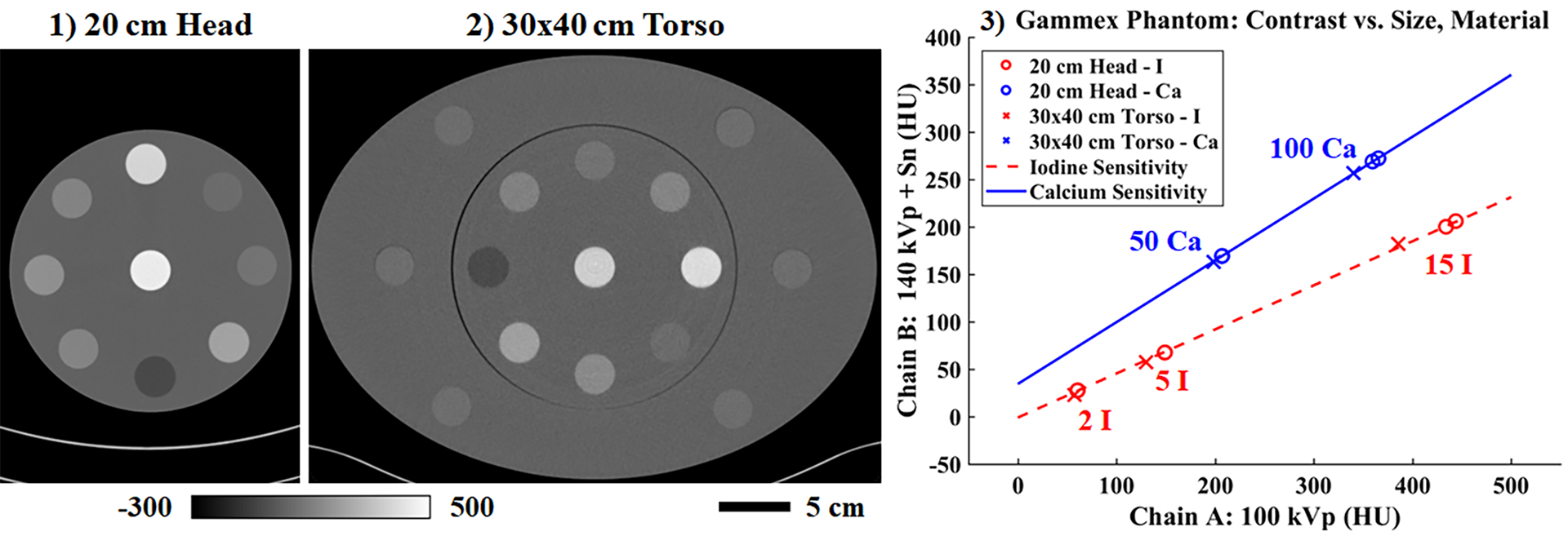
Reconstructed attenuation values in the Gammex phantom measured in the 20 cm head phantom (1) and then again in the 30×40 cm torso phantom (2) (chain A shown, 10 cm slice thickness). (3) Beam hardening effects are seen to reduce reconstructed intensity values for known concentrations of iodine (I) and calcium (Ca; units: mg/mL); however, the linear dependence of attenuation on material concentration is preserved. Calibration bar units: HU.

Spectral extrapolation results for the Gammex torso phantom and a second material rod configuration are shown in Fig. 9. Following the format of previous figures, contrast differences are shown between chains A and B (2) and between chain B and the output of the PLTF (3) and then the CNN (4). The material rods are numbered in (1) with the corresponding materials labeled in Table 3 along with their measured attenuation differences. Across all material rods, the PLTF generally reduces the chain B contrast estimation error relative to the initial contrast difference between chains A and B (exceptions: rod 3, “Blood”; rods 10, 12, 13, and 15, “Muscle”). For rods within the training mask (1–9), the CNN explicitly preserves the chain B contrast (maximum error by magnitude, 0.33 HU). For rods outside of the training mask and in the training halo (10–15), however, the CNN spectral extrapolation results are less consistent, particularly for the 2 and 15 mg/mL iodine rods (contrast estimation errors: −17.34 and −28.89 HU, respectively). Compared with the much smaller average errors seen in the testing data (Fig. 7, Table 2), these phantom results appear to confirm the significance of feature-contrast relationships in correctly inferring spectral contrast within the training halo, since such relationships are completely ambiguous within the Gammex phantom.

Fig. 9.

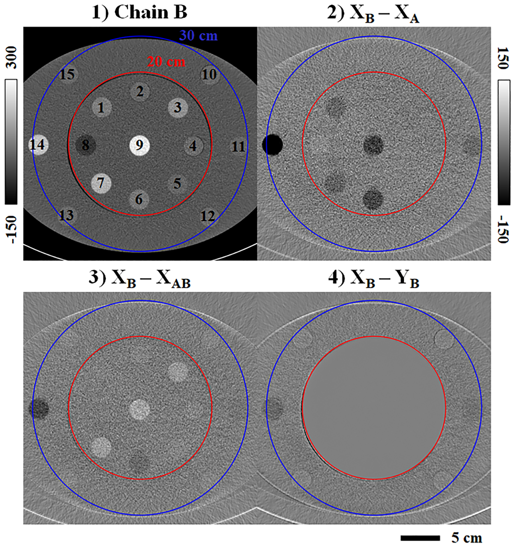
Spectral extrapolation applied to the Gammex Multi-Energy CT phantom. (1) Chain B CT data (3 cm slice thickness) with labeled material rods (legend in Table 3). The ReconCT reconstruction is shown prior to network evaluation. (2) Initial contrast difference between chain B and chain A. (3) Chain B contrast estimation error following the PLTF. (4) Chain B contrast estimation error following the CNN. Calibration bar units: HU.

Table 3.

Gammex phantom spectral contrast measurements (HU).

ROI	Material	XB	XB - XA	XB - XAB	XB - YB	Iodine(a) (YA, YB)
1	Blood Iodine (2 mg/mL)	67.49	−32.11	−1.00	−0.26
2	Muscle	33.96	−8.39	1.37	−0.08
3	Blood	104.45	−9.76	27.08	0.25
4	Muscle	35.99	−6.02	3.31	0.23
5	Brain	28.75	−1.92	3.70	0.30
6	Iodine (5 mg/mL)	58.29	−68.74	−26.82	−0.13	5.00(b)
7	Calcium (50 mg/mL)	160.39	−37.60	31.86	0.04
8	Adipose	−55.63	9.97	−8.04	−0.12
9	Calcium (100 mg/mL)	257.90	−78.20	39.57	0.33
10	Muscle	37.63	−4.21	4.53	1.22
11	Iodine (2 mg/mL)	28.79	−27.98	−13.61	−17.34	0.80
12	Muscle	38.09	−3.55	5.22	2.28
13	Muscle	38.81	−2.12	6.44	2.55
14	Iodine (15 mg/mL)	191.55	−205.07	−69.03	−28.89	12.90
15	Muscle	37.76	−0.43	6.98	3.49
16	Iodine (2 mg/mL)	28.79	−24.21	−8.87	−16.05	0.37
17	Iodine (15 mg/mL)	191.55	−203.11	−67.84	−27.26	12.88

Notes: Bold text indicates minimum HU errors by magnitude relative to X_B. Underlined text indicates assumed values.

^(a)Units of mg/mL.

^(b)Reference iodine measurement.

ROIs 1–9: within 20 cm mask. 10–15: within 30 cm mask. 16–17: extended 50 cm FoV.

Following the results in Figs. 5–6, which show that spectral extrapolation smooths image features, Fig. 10 quantifies the impact of this smoothing on spatial resolution measured within the chain B data. High contrast material rods (>190 HU) located within the chain B training mask (100 mg/mL Ca; black, cyan), mostly within the training halo (15 mg/mL I; magenta), and beyond the training halo (extended chain B FoV; 15 mg/mL I; green) are chosen for MTF measurements (colored, square ROIs). Comparing the resultant MTF curves, spatial resolution is very similar within the chain B training mask and the chain B halo (10% modulation transfer: 4.91–5.24 lp/cm), even when the phantom position is shifted 6 cm from the center of the scanner FoV (panel (1) vs. (2)). However, some loss of spatial resolution is observed in the extended chain B FoV: the spatial frequency at 10% modulation transfer decreases from 5.15 lp/cm (magenta box) to 4.15 lp/cm (green box) when the 15 mg/mL iodine rod is moved from the training halo (1) into the extended FoV (2). Consulting Table 3, the spectral extrapolation errors for the 2 and 15 mg/mL I rods are similar when the rods are moved from the training halo (−17.34 HU, ROI 11; −28.89 HU, ROI 14) to the extended FoV (−16.05 HU, ROI 16; −27.26 HU, ROI 17). Material decomposition calibrated by the 5 mg/mL iodine rod in the training mask (ROI 6) yields iodine measurements of 0.80, 12.90 mg/mL (training halo) and 0.37, 12.88 mg/mL (extended FoV) for the 2 and 15 mg/mL iodine rods, respectively. Similar errors for both rod configurations confirm the ambiguity of feature-contrast relationships in the Gammex phantom, as proximity to the chain B mask does not strongly influence extrapolation performance.

Fig. 10.

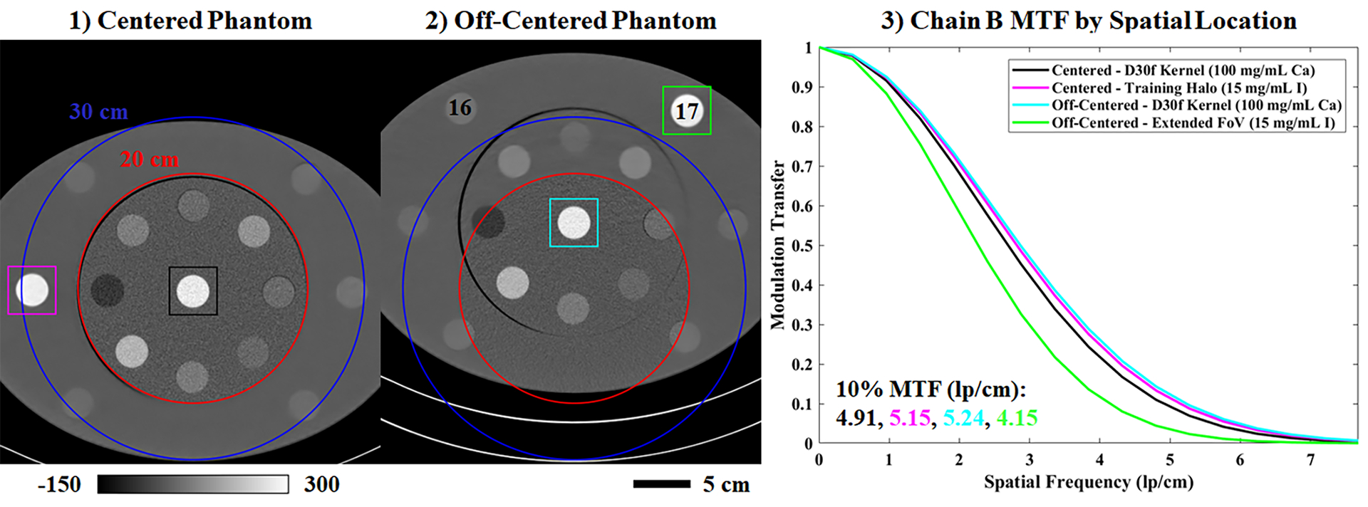
Spatial resolution following spectral extrapolation. (1) Chain B CT data (3 cm slice thickness) matching Fig. 9. The phantom is centered with respect to the chain B FoV. (2) Chain B CT data from a second scan where the phantom is off-centered, positioning two iodine rods outside of the training halo (legend in Table 3). (3) Color-coded, axial MTF measurements taken in the square ROIs denoted in (1) and (2). Calibration bar units: HU.

3.C. Deep-learning enhanced workflow

Following network training and testing, spectral post-processing was applied to one of the testing data sets following a “standard” clinical workflow (Fig. 11, row 1) and the proposed workflow augmented with spectral extrapolation (row 2). Fig. 11.3 compares 50 keV monoenergetic images synthesized within the two workflows. SNR values are reported in several matching ROIs (yellow circles, text) in the liver, right kidney, left kidney, and muscle for comparison. Because the errors in mean intensity between the two workflows are below 9 HU, reduced SNR values in the extrapolation results mostly indicate increased noise in the monoenergetic images produced with spectral extrapolation. This is somewhat counterintuitive given the image smoothing associated with spectral extrapolation in the training halo (Fig. 11.2). Fig. 11.4 demonstrates the quantitative accuracy of material decomposition into iodine (red) and virtual non-contrast (VNC, gray) images within the training halo. Yellow circles and text denote iodine concentration measurements in several matching ROIs in the liver, right kidney, and left kidney. The maximum measured discrepancy between the ROIs is 0.66 mg/mL of iodine measured in the hypo-enhancing, cystic liver lesion (left green box). This discrepancy does not appear to indicate a general bias in the extrapolation of low contrast structures as the discrepancy measured in a low contrast kidney cyst (right green box) is only 0.09 mg/mL of iodine. Furthermore, similar extrapolation errors are measured in the right (2.65 vs. 2.09 mg/mL) and left kidney ROIs (6.95 vs. 6.54 mg/mL) despite a 2.6x difference in reference iodine concentrations. Interestingly, for every pair of ROIs, the magnitude of the estimated iodine concentration is lower than the magnitude of the reference iodine concentration.

Fig. 11.

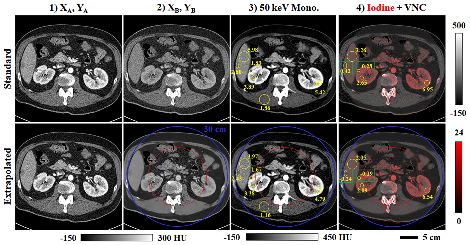
Spectral processing of extrapolated data (Test Case 5, Fig. 7). (1) Analytical reconstruction for chain A before (first row) and after (second row) application of the spectral extrapolation network. (2) Analogous data for chain B. (3) 50 keV monoenergetic images including matching ROIs (yellow circles, text) denoting SNR measurements. (4) Iodine decompositions (red color map, mg/mL) overlaid on complementary virtual non-contrast (VNC) images (calibration bars shown at right). Matching regions of interest (yellow circles, text; green boxes) compare mean reference (first row) and extrapolated (second row) iodine concentrations measured in the liver and kidneys.

Lastly, Fig. 12 summarizes contrast uniformity measurements to confirm the suitability of spectral extrapolation for performing quantitative spectral measurements. Neglecting the potential effects of beam hardening in the 140 kVp chain B data, contrast enhancement in the liver parenchyma is expected to be roughly uniform. Yellow ROIs and text in Fig. 12.1 report mean enhancement values measured within the chain B training mask (20 cm), within the training halo (20–30 cm), and in the extended FoV (30+ cm). For the chain B data, the maximum measurement discrepancy is 7.2 HU, or ~8% of the reference enhancement measured in the abdominal aorta (93.4 HU). Following material decomposition, the maximum discrepancies increase to ~12% in the iodine map (abdominal aorta: 75 HU) and the VNC image (59 HU) for the same ROIs. Comparing the iodine measurement discrepancies here (<1 mg/mL) and in Fig. 11.4 (max error: 0.66 mg/mL) with the iodine measurement errors seen in the Gammex phantom (Table 3, >1 mg/mL) suggests that spectral extrapolation performance is better in patient data than it is in Gammex phantom data. In future work, this could recommend phantom studies during network testing as a means to assess baseline performance.

Fig. 12.

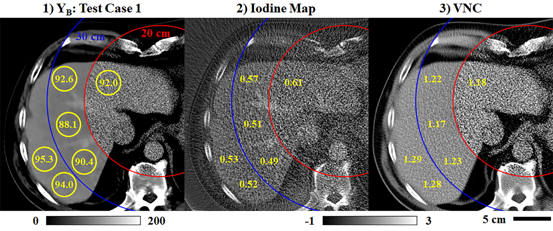
Uniformity of spectral measurements (Test Case 1, Fig. 7). (1) Extrapolated chain B data including several ROIs (yellow circles) where mean contrast measurements are reported (yellow text, HU calibration bar). Measurements span the training mask (red circle, 20 cm), the training halo (blue circle, 20–30 cm), and the extended FoV (30+ cm). (2–3) Analogous measurements taken in the iodine map (2) and the VNC image (3), normalized by the contrast measured in the abdominal aorta for each image (calibration bar: −1x to 3x abdominal aorta contrast).

4. Discussion and Conclusions

In this work we have proposed and demonstrated spectral extrapolation, an image domain procedure which uses a network composed of a PLTF and a CNN to robustly estimate spectral contrast over the complete FoV of dual-source, dual-energy x-ray CT data acquired with a clinical scanner. Exploiting the spatial invariance of our network, we were able to train it with existing, truncated dual-source, dual-energy CT data by artificially limiting the chain B FoV further, providing a halo where the true chain B data is known. This training procedure explicitly emulates the extrapolation of spectral contrast beyond the nominal 33 cm FoV for chain B, achieving the goal of extrapolating spectral contrast to the full FoV of chain A (50 cm; Figs. 10 and 12). Working in the gap in standard clinical workflows between data reconstruction and spectral post-processing, a further strength of our proposed method is that it yields a trained network which could be immediately integrated into existing clinical workflows without increases in workflow complexity.

While our primary goal in pursuing spectral extrapolation is to enable spectral processing over a larger FoV, increasing the value of dual-energy CT when scanning large patients, there are a number of closely related applications which may also benefit from spectral extrapolation. For instance, accurate spectral contrast estimation will likely improve model-based approaches to image reconstruction and artifact corrections by improving data consistency with an underlying forward model. Advanced cardiac applications such as dual-source, dual-energy cardiac CT, which typically compromise between spectral contrast and temporal resolution, could be enhanced by robustly estimating spectral contrast at quarter-rotation temporal resolution. The accuracy of radiotherapy calculations derived from extended dual-energy information²⁵ may also be improved. If spectral extrapolation becomes a proven technique, it may even lead to relaxation of CT system design parameters, enabling low-dose interior tomography for cardiac imaging or cost-effective, high-resolution photon counting CT. Such photon counting CT systems could potentially operate a standard, full FoV energy-integrating imaging chain in tandem with a photon counting imaging chain with a smaller FoV and pixel pitch.⁴

There are several important limitations of our work to be addressed in future studies. First, we demonstrate that spectral extrapolation is possible, but we do so within the limited scope of a single data acquisition and reconstruction protocol and with a somewhat limited amount of training data. These conditions establish a proof-of-concept, but do not establish spectral extrapolation as an all-purpose technique applicable under other imaging conditions or when targeting other organ systems. Performance limits for spectral extrapolation, such as the 0.66 mg/mL iodine error seen in Fig. 11, will have to be established in a task-dependent manner prior to its wide-spread application. Ultimately, greater standardization of clinical workflows and the quality-assurance procedures used to regulate them will likely be required for compatibility with this and many other deep-learning based algorithms. Second, our current approach to spectral extrapolation visibly smooths the chain B image data outside of the training mask (Figs. 5–6, 10–12). This smoothing is a result of matching independent noise observations between the chain A data and the known chain B data used as training labels. It is also a well-documented side effect of minimizing a mean-squared-error cost function during network training. This smoothing could be considered a positive feature: it is visually obvious where the spectral contrast is estimated and where it is known. Practically, however, alternative cost functions should be investigated in future work to better preserve image structure, to promote diagnostic confidence, and to maximize compatibility with down-stream spectral processing (e.g. to better control the noise level in monochromatic images, Fig. 11.3). Third, we claim that a CNN’s ability to learn complex feature-contrast relationships across multiple resolution levels is the reason why the spectral extrapolation problem may be better conditioned than it first appears and why extrapolation performs somewhat poorly on simple phantom data relative to patient data; however, the deep-learning “black box” makes it somewhat difficult to understand feature-contrast relationships and their limitations in practice. Future work will require the application of “explainable AI” techniques such as occlusion mapping to better understand the performance and limitations of spectral extrapolation.^26,27 Finally, on a technical note, we have proposed a low-pass residual connection strategy for modifying a U-net to explicitly couple chain A and B data during spectral processing (Eqs. 3–4, Fig. 3), but further comparison with a classic residual connection (adding X₀ to the network output instead of X_LP) has shown marginal changes in the validation performance of the trained network. Future work in the application of machine learning algorithms to multi-channel CT data should more thoroughly investigate optimal data normalization strategies.

Here, we have worked exclusively in the image domain; however, future work should compare reprojections of the extrapolated data with the original projection data for each imaging chain. The projection data acquired for chain B does not allow accurate analytical reconstruction outside of the chain B FoV, but the line integrals which are sampled by chain B are complete and should be consistent with reprojections through extrapolated data. Such consistency measures will lend confidence to the fidelity of spectral extrapolation on a patient-by-patient basis and may even allow the assignment of confidence intervals to extrapolated data or further improvements to spectral extrapolation accuracy. We speculate that the close ties between sparse representation, feature-contrast relationships, multi-resolution analysis, and deep learning may even yield a new paradigm for compressive sensing in spectral CT data acquisition and reconstruction, making use of spectral extrapolation to robustly estimate missing data.

References

- 1.Ohnesorge B, Flohr T, Schwarz K, Heiken J, Bae K. Efficient correction for CT image artifacts caused by objects extending outside the scan field of view. Medical physics. 2000;27(1):39–46. [DOI] [PubMed] [Google Scholar]
- 2.Flohr T, Bruder H, Stierstorfer K, Petersilka M, Schmidt B, McCollough C. Image reconstruction and image quality evaluation for a dual source CT scanner. Medical physics. 2008;35(12):5882–5897. [DOI] [PMC free article] [PubMed] [Google Scholar]
- 3.Stierstorfer K, Rauscher A, Boese J, Bruder H, Schaller S, Flohr T. Weighted FBP—a simple approximate 3D FBP algorithm for multislice spiral CT with good dose usage for arbitrary pitch. Physics in Medicine & Biology. 2004;49(11):2209. [DOI] [PubMed] [Google Scholar]
- 4.Yu Z, Leng S, Li Z, Halaweish AF, Kappler S, Ritman EL, McCollough CH. How low can we go in radiation dose for the data-completion scan on a research whole-body photon-counting CT system. Journal of computer assisted tomography. 2016;40(4):663. [DOI] [PMC free article] [PubMed] [Google Scholar]
- 5.Clark D, Badea C. Spectral data completion for dual-source x-ray CT. Paper presented at: Medical Imaging 2019: Physics of Medical Imaging2019. [Google Scholar]
- 6.Ronneberger O, Fischer P, Brox T. U-net: Convolutional networks for biomedical image segmentation. Paper presented at: International Conference on Medical Image Computing and Computer-Assisted Intervention2015. [Google Scholar]
- 7.Wang G A perspective on deep imaging. Ieee Access. 2016;4:8914–8924. [Google Scholar]
- 8.Lucas A, Iliadis M, Molina R, Katsaggelos AK. Using deep neural networks for inverse problems in imaging: beyond analytical methods. IEEE Signal Processing Magazine. 2018;35(1):20–36. [Google Scholar]
- 9.Chen H, Zhang Y, Kalra MK, Lin F, Chen Y, Liao P, Zhou J, et al. Low-dose CT with a residual encoder-decoder convolutional neural network. IEEE transactions on medical imaging. 2017;36(12):2524–2535. [DOI] [PMC free article] [PubMed] [Google Scholar]
- 10.Han Y, Ye JC. Framing U-Net via deep convolutional framelets: Application to sparse-view CT. IEEE transactions on medical imaging. 2018;37(6):1418–1429. [DOI] [PubMed] [Google Scholar]
- 11.Missert AD, Yu L, Leng S, Fletcher JG, McCollough CH. Synthesizing images from multiple kernels using a deep convolutional neural network. Medical physics. 2019. [DOI] [PubMed] [Google Scholar]
- 12.Zhang W, Zhang H, Wang L, Wang X, Hu X, Cai A, Li L, et al. Image domain dual material decomposition for dual‐energy CT using butterfly network. Medical physics. 2019;46(5):2037–2051. [DOI] [PubMed] [Google Scholar]
- 13.Chen Z, Li L. Preliminary research on multi-material decomposition of spectral CT using deep learning. Paper presented at: Proceeding of the 14th International Meeting on Fully Three-Dimensional Image Reconstruction in Radiology and Nuclear Medicine2017. [Google Scholar]
- 14.Clark D, Holbrook M, Badea C. Multi-energy CT decomposition using convolutional neural networks. Paper presented at: Medical Imaging 2018: Physics of Medical Imaging 2018. [Google Scholar]
- 15.Poirot MG, Bergmans RH, Thomson BR, Jolink FC, Moum SJ, Gonzalez RG, Lev MH, et al. physics-informed Deep Learning for Dual-energy computed tomography image processing. Scientific reports. 2019;9(1):1–9. [DOI] [PMC free article] [PubMed] [Google Scholar]
- 16.Shi Z, Li J, Li H, Hu Q, Cao Q. A Virtual Monochromatic Imaging Method for Spectral CT Based on Wasserstein Generative Adversarial Network With a Hybrid Loss. IEEE Access. 2019;7:110992–111011. [Google Scholar]
- 17.Liu G, Reda FA, Shih KJ, Wang T-C, Tao A, Catanzaro B. Image inpainting for irregular holes using partial convolutions. Paper presented at: Proceedings of the European Conference on Computer Vision (ECCV)2018. [Google Scholar]
- 18.Wei Y, Yuan Q, Shen H, Zhang L. Boosting the accuracy of multispectral image pansharpening by learning a deep residual network. IEEE Geoscience and Remote Sensing Letters. 2017;14(10):1795–1799. [Google Scholar]
- 19.Cheng Z, Yang Q, Sheng B. Deep colorization. Paper presented at: Proceedings of the IEEE International Conference on Computer Vision2015. [Google Scholar]
- 20.American_College_of_Radiology. Quality Control: CT (Revised 12-12-19). https://accreditationsupport.acr.org/support/solutions/articles/11000056188-quality-control-ct. Accessed February 25th, 2020.
- 21.Gammex. CT QA Solutions: Multi-Energy CT Phantom. https://www.sunnuclear.com/uploads/documents/datasheets/gammex/MultiEnergyCTScanners_D071019.pdf. Accessed January 29th, 2020.
- 22.Maas AL, Hannun AY, Ng AY. Rectifier nonlinearities improve neural network acoustic models. Paper presented at: Proc. icml 2013. [Google Scholar]
- 23.Kingma DP, Ba J. Adam: A method for stochastic optimization. arXiv preprint arXiv:14126980. 2014. [Google Scholar]
- 24.Siewerdsen JH, Wojciech Z, Xu J. Chapter 4: Cone-beam CT image quality In: Shaw CC, ed. Cone beam computed tomography. Taylor & Francis; 2014:37–58. [Google Scholar]
- 25.van Elmpt W, Landry G, Das M, Verhaegen F. Dual energy CT in radiotherapy: current applications and future outlook. Radiotherapy and Oncology. 2016;119(1):137–144. [DOI] [PubMed] [Google Scholar]
- 26.Gunning D, Aha DW. DARPA’s Explainable Artificial Intelligence Program. AI Magazine. 2019;40(2):44–58. [Google Scholar]
- 27.Zeiler MD, Fergus R. Visualizing and understanding convolutional networks. Paper presented at: European conference on computer vision2014. [Google Scholar]