Comparison of Parameter Optimization Methods for Quantitative Susceptibility Mapping

Abstract

Purpose:

Quantitative susceptibility mapping is usually performed by minimizing a functional with data fidelity and regularization terms. A weighting parameter controls the balance between these terms. There is a need for techniques to find the proper balance that avoids artifact propagation and loss of details. Finding the point of maximum curvature in the L-curve is a popular choice, although slow, often unreliable when using variational penalties, and tends to yield over-regularized results.

Methods:

We propose two alternative approaches to control the balance between the data fidelity and regularization terms: 1) searching for an inflection point in the log-log domain of the L-curve, and 2) comparing frequency components of QSM reconstructions. We compare these methods against the conventional L-curve and U-curve approaches.

Results:

Our methods achieve predicted parameters that are better correlated with RMSE, HFEN and SSIM-based parameter optimizations than those obtained with traditional methods. The inflection point yields less over-regularization and lower errors than traditional alternatives. The frequency analysis yields more visually appealing results, although with larger RMSE.

Conclusion:

Our methods provide a robust parameter optimization framework for variational penalties in QSM reconstruction. The L-curve based zero-curvature search produced almost optimal results for typical QSM acquisition settings. The frequency analysis method may use a 1.5–2.0 correction factor to apply it as a standalone method for a wider range of SNR settings. This approach may also benefit from fast search algorithms such as the binary search to speed-up the process.

Introduction

Quantitative Susceptibility Mapping (QSM) is an MRI-based technique that estimates subtle variations in tissue magnetic susceptibility. Susceptibility distributions are inferred from the phase of complex Gradient Recalled Echo (GRE) images. These phases are proportional to changes in the local magnetic field generated by susceptibility sources in the presence of the main external magnetic field¹. The calculation of the susceptibility distribution is an ill-posed inverse problem. The dipole kernel used in the susceptibility-to-field model has a simple formulation in frequency space, where a zero-valued conical surface cancels all frequency components and significantly dampens the data close to this surface^2,3. A straightforward division would yield undetermined divisions by zero, and large noise-amplification effects^4,5. Most of the state-of-the-art QSM techniques rely on solving the inverse problem by the optimization of a cost function^6–8. This function commonly consists of two terms: data fidelity and regularization. The data fidelity term computes an error metric between the estimated susceptibility distribution and the measured phase. The regularization term includes prior knowledge about the solution, like smoothness, sparsity in a given domain, piece-wise smoothness, or any constraint that could ensure the existence of a unique and well-conditioned reconstruction. Both terms are balanced employing a Lagrangian weight that needs to be fine-tuned for optimal results. If the Lagrangian weight multiplies the regularization term, too small values might lead to noise amplifications due to the instability of the inverse problem, whereas large values would yield over-regularized solutions, with little anatomical detail and/or with low fidelity to the acquired data. The optimal regularization weight depends on the noise level and the acquisition settings. Reconstructions are sensitive to small changes in this parameter, and the optimal parameter may change for different datasets.

Finding the proper regularization weight is usually a challenging and time-consuming heuristic task. The inverse problem must be solved several times, with different weights, in search of the optimal value. Empirical visual assessment remains as one of the most reliable methods for QSM, but it requires an expert to accurately perform the evaluation. Although several strategies have been proposed in the inverse problems literature^9–11, the analysis of the L-Curve¹² is the most popular alternative being used for QSM¹³. In a nutshell, this analysis looks for the optimal trade-off point between the costs of the data-fidelity and regularization terms. Originally proposed for Tikhonov regularization problems, the optimal trade-off is found at the corner of an L-shaped curve that is created by both costs. The maximum point of curvature usually matches with this corner. Since Tikhonov-based regularizers exploit smoothness of the solutions, variational penalties (TV, TGV, etc.) are among the most popular regularizers for QSM, due to their edge preservation properties. In this case, instead of a sharp L-shaped curve, the cost functions yield a smooth curve, often with unexpected behaviors^14,15. The curvature near the optimum value changes slowly, with point-to-point deviations introducing large effects in the curvature calculation¹⁶. This makes the maximum curvature search not robust enough for fine-tuning, providing only an order of magnitude estimation in most scenarios. In addition, it has been observed that L-curve-based optimization usually yields over-regularized solutions¹⁷. A different approach using both the data fidelity and reconstruction costs is present in the U-Curve¹⁷ analysis, with promising results. For these reasons, new strategies for optimal parameter fine-tuning must be developed for QSM applications. In this paper, we present two new alternatives to achieve improved robustness and obtain visually appealing results. We compare these new methods with the existing L-curve and U-curve approaches, which so far has not been tested for QSM reconstructions.

Methods

We formulate the following reconstruction problem to estimate the susceptibility distribution, χ^13,18:

$$\mathit{\text{argmi}}{n}_{\chi }\frac{1}{2}\Vert W\left(F^{H}DF\chi -\Phi \right){\Vert }_2^2+\alpha \Omega \left(\chi \right),$$ (1)

or the nonlinear data consistency variant^19,20:

$$\mathit{\text{argmi}}{n}_{\chi }\frac{1}{2}{\Vert W\left(e^{i{F}^{H}DF\chi }-e^{i\Phi }\right)\Vert }_2^2+\alpha \Omega \left(\chi \right),$$ (2)

where W is a noise-whitening weight, proportional to the signal magnitude. α is a Lagrangian weight that must be fine-tuned for optimal results and multiplies a regularization term Ω(χ). Φ is the measured GRE phase, F is the Fourier operator with its adjoint F^H, and D is the dipole kernel in the frequency-domain^2,3:

$$D=\gamma H_{0}TE\left(\frac{1}{3}-\frac{k_z^2}{k^2}\right),$$ (3)

where H₀ is the strength of the main magnetic field, TE the echo time and γ the gyro-magnetic ratio. For simplicity, we use Total Variation as regularizer^21,22:

$$\Omega \left(\chi \right)=|\nabla \chi {|}_1,$$ (4)

In an L-curve optimization scheme, the cost associated to each term is calculated for different α values, and then the curvature is calculated as^12,13:

$$\kappa =\frac{C\prime R″-R\prime C″}{{\left(C{″}^2+R{″}^2\right)}^{3/2}},$$ (5)

To calculate the first and second derivatives of the data consistency cost C (C’ and C”) and the derivatives of the regularization cost R (R’ and R”), a typical strategy is to perform a spline interpolation.

In the case of variational penalties, there is a soft curvature change that prevents a precise estimation of the point with maximum curvature. A coarse α optimization is feasible using this method for undersampled L-curve representations. Recent high-speed solvers^13,20,22 allow a denser sampling of the L-curve (more than a couple of results per order of magnitude), for a more precise parameter optimization. In this scenario, we present two new strategies to find the optimal α parameter, as follows.

High-density L-curve analysis

Variational penalties present a smooth L-shaped linear graph in the logarithm space, which is better represented by an S-shape. Empirically, we propose to use the main inflection of the curve to optimize the regularization weight (i.e. find the point where the sign of the curvature changes). This point may be calculated using Eq. (5), searching for the first zero-crossing point starting from a large regularization weight value (to avoid instabilities due to the effects of the streaking artifacts).

The U-curve analysis

The U-curve method is widely used to find a range of suitable optimal parameters in inverse problems, such as inverse electromagnetic modeling, super-resolution, and others^17,23,24. However, it has not been tested yet for QSM problems. This method minimizes a convex functional defined by the sum of the reciprocates of the data consistency and regularization costs (C and R, as defined for the L-curve)¹⁷:

$$U=\frac{1}{C}+\frac{1}{R},$$ (6)

As such, the U-curve has been proposed as a more efficient alternative to the L-curve analysis.

Susceptibility-Frequency Equalization

We propose a method based on the inspection of high-frequency coefficients of the reconstructed susceptibility maps. In image reconstruction or restoration problems, analyzing the frequency components may reveal noise amplifications or attenuations for given frequencies. In MRI, this was explored using the Error Spectrum Plot²⁵, which creates a vectorized error metric to assess the accuracy of reconstructions for consecutive rings or shells around the DC component. This idea was further developed for QSM, changing the spherical shells into double-coned surfaces, following the characteristics of the dipole kernel²⁶. If we analyze the dipole kernel in the frequency-domain, the coefficients in spherical coordinates are given by^2,3:

$$D\left(\theta \right)=\gamma H_{0}TE\left(\frac{1}{3}-{\text{cos}}^2\theta \right),$$ (7)

This means that the coefficients of the dipole kernel only depend on θ, the angle from the main field axis. If we divide by γH₀TE, the dipole kernel coefficients start at −2/3 along the main field axis (θ=0°), reaching up to 1/3 in the orthogonal plane (θ=90°), being zero at the “magic angle”. We will use this normalized formulation in the following sections to analyze dipole kernel coefficients.

Using Parseval’s theorem, the data consistency term may be expressed in the Fourier domain, with equivalent results. In this representation, dipole kernel coefficients act as weights that promote consistency between the true or ideal susceptibility distribution and the optimized estimation. This means that, in frequency space, coefficients multiplied by small dipole kernel coefficients show large regularization effects. As seen in Figure 1, this property shapes the frequency coefficients of the reconstructions depending on the regularization weights. Under-regularized results present amplification of the coefficients close to the magic angle (noise amplification that also results in streaking artifacts), whereas over-regularized results attenuate these coefficients. By visual inspection of the Power Spectrum (magnitude of the frequency coefficients), optimal results seem to be achieved when high-frequency coefficients have similar local mean values inside spherical shell sections.

Figure 1.

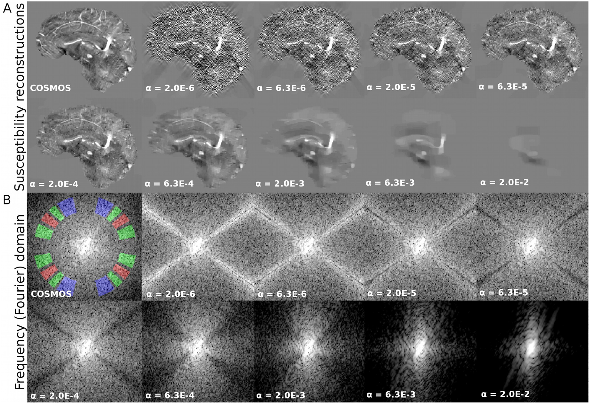
QSM reconstructions (A) and their Fourier transforms (B) for different regularization weights. Proposed ROI masks are represented in red (M₁), green (M₂) and blue (M₃) overlying the COSMOS frequency ground-truth.

Given this observation, we propose to use masks (M) in the frequency-domain that define certain regions of interest (ROI) to characterize the ”amplitude” (A) of the coefficients. By comparing these regions, we can determine the amplification or attenuation associated with the reconstruction using a particular regularization weight. The estimation of the mask amplitude may be performed efficiently by taking the L2-norm of the complex coefficients of the Fourier Transform of the susceptibility reconstructions, or by averaging the Power Spectrum values. For simplicity, we used the average of the Power Spectrum values in our study. The proposed optimal regularization weight is the one that minimizes the normalized squared difference in mask amplitudes between two ROIs, A_i and A_j:

$${\zeta }_{ij}={\left(\frac{A_i-A_j}{A_i+A_j}\right)}^2,$$ (8)

The denominator in Eq. (8) penalizes solutions with similar amplitudes for both masks, but that were attenuated by over-regularization. This metric behaves in a convex manner in a wide range around the optimal parameter. Note that if the curves described by the evolution of the amplitude of two different regions as a function of the regularization weight intercept, then the ζ functional is minimized at this point (Figure 2E).

Figure 2.

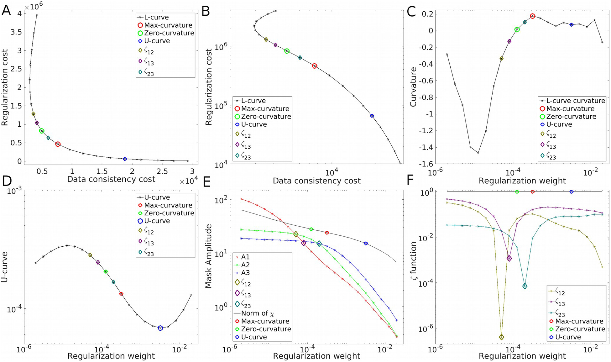
Parameter optimization strategies on the COSMOS-brain simulations at SNR=40. The L-curve in linear (A) and logarithm (B) representations, with its curvature (C). The U-curve (D). Frequency analysis using the amplitude estimations A₁, A₂ and A₃ (E) and the ζ cost functions (F).

In this study we used three masks defined by the absolute values of the dipole kernel’s frequency coefficients (which select a volume between two double-shaped cones): M₁ = 0<D<0.085, M₂ = 0.15<D<0.3 and M₃ = 0.35<D<0.6. In all three masks, the frequency radial ranges were set from 0.65 1/mm to 0.95 1/mm (see Supporting Information Figure S1 for a 3D render of these masks) to avoid high coefficient values due to structural information. These threshold values were found empirically. The first mask M₁ covers a volume that includes coefficients inside the magic cone and its surroundings, which are more prone to noise-amplification. The second mask M₂ was chosen as a region contiguous to M₁, without coefficients too prone to be affected by noise-amplification (i.e. are not divided by too small dipole kernel coefficients), but should still be sensitive to attenuation. As seen in Figure 1, the volume affected by the amplification of coefficients (under-regularization regime) is constrained, whereas the volume affected by attenuation (over-regularization regime) is larger, and depends on the regularization weight. The third mask M₃ provides a region largely insensitive to noise-amplification, and even less sensitive to attenuation. M₃ was also chosen to avoid frequency coefficients on (or close to) the XY plane and the X = Y = 0 vertical line, as these coefficients may contain relatively high coefficients values due to zero-padding in the image domain and other structural effects.

Given that these frequency masks were defined based on the frequency information of a COSMOS reconstruction, we expect them to work for a wide range of targets in human brain QSM applications. Adjustments should be made if the brain-tissue mask changes significantly, or if maps are calculated for body regions other than the brain. Whereas minor head angulations should not be an issue, voxel asymmetry should be analyzed (we include an in vivo acquisition with highly anisotropic voxels with the default frequency masks and modified masks as an example).

Experimental setup

We conducted synthetic numerical simulations and in vivo experiments to validate the two proposed methods, and to compare them against the commonly used L-shaped (maximum curvature) and the U-curve methods. QSM reconstructions were performed using the functionals described in (1) and (4), with an ADMM based solver (FANSI Toolbox)²⁰. The maximum number of iterations was set to 300, and the convergence tolerance was set to less than 0.1% signal update between iterations, for all experiments. All routines were run in MATLAB (The Mathworks Inc., Natick, MA, USA), on an Acer Predator laptop computer (Intel i7 6700HQ processor with 64GB RAM). As previously reported, all internal parameters introduced by the ADMM solver were set to fixed values or fixed proportions in relation to the main regularization weight (α)^20,27. In particular, the Lagrangian weight related to the Total Variation subproblem was chosen as μ₁ = 100α. The Lagrangian weight related to the Data Fidelity term subproblem (μ₂) was set to 1.0.

COSMOS-brain numerical simulations

A noise-corrupted field map was forward-simulated using the 12-head-orientations COSMOS reconstruction²⁸ included in the 2016 QSM Reconstruction Challenge dataset²⁹ from spoiled 3D-GRE scans acquired on a 3T Siemens Tim Trio system using a 32-channel head-coil with 1.06-mm isotropic voxels, 15-fold Wave-CAIPI acceleration³⁰, 240×196×120 matrix size, echo time (TE)/repetition time (TR)=25/35 ms, flip angle=15°. We forward simulated the phase data for different peak signal-to-noise ratio (SNR) values, from 16 to 256, in a dyadic sequence. Since only local phases were simulated, no unwrapping or background field removal methods were applied.

QSM reconstructions were evaluated with Root Mean Square Error (RMSE), High-Frequency Error Norm (HFEN) and the Structural Similarity Metric (SSIM, with default K = [0.01, 0.03] and L = 255 parameters)^29,31, with respect to the COSMOS (ground-truth) acquisition.

In vivo data

A single axial head-orientation GRE data (same imaging parameters as those described above) was also provided in the context of the 2016 QSM Reconstruction Challenge.

Two additional 3T in vivo datasets are provided as Supporting Information, as examples of different SNR, voxel size ratio and vendors.

We also include an acquisition performed with a 7T Siemens MAGNETOM, using a 32-channel Nova head-array. TE/TR=9/20ms, flip angle=10°, bandwidth=120 Hz/pixel, fully-sampled with 504×608×88 matrix and 0.33×0.33×1.25-mm3 voxel size. Total acquisition time of 17:30 min. Phase unwrapping and harmonic phase removal were performed using HARPERELLA³² and VSHARP³³ (R0=25mm) algorithms, respectively.

In addition, to provide quantitative results with the mentioned error metrics (available only for simulations), we conducted a visual assessment of the quality of all the reconstructions. This assessment was performed by the authors using the following visibility criteria: Presence of streaking artifacts; image texture (i.e. reject too smooth or cartoon-like images); noise amplification; and preservation of image contrast between structures. In this analysis, solutions with small amount of noise were preferred over smooth structures or lack of texture, following the concept of comfort noise³⁴.

All in vivo acquisitions were performed with fully informed consent, and under approval of the local Ethics Committee.

Results

COSMOS-brain numerical simulations

As the primary example, we present the results achieved for SNR=40 in Figure 1. We explored the results within 4 orders of magnitude, along with their Fourier Transforms. Visual inspection confirms that over-regularized results have strongly attenuated frequency coefficients following the shape of the magic cone, whereas under-regularized results present noise amplification, especially around the magic angle. The L-curve and its logarithm representation are displayed in Figures 2A and 2B, respectively. Note the S-shaped look of the curve in the logarithmic domain. The smooth nature and difference in scales make it hard to find the L-corner point (maximum curvature, marked with a red circle). The inflection point of the logarithmic graph is easier to identify, validated by the curvature graph (Figure 2C). The U-curve analysis returned the largest regularization weight value. By using the three masks (in red, green and blue, overlying the Fourier Transform of the COSMOS data) we inspected the evolution of the amplitude of the frequency coefficients. The graph in Figure 2E shows three points where the amplitudes are equal between two masks (i.e. the amplitude curves intercept). The region that covers the magic cone suggests smaller regularization weights than when using only external masks (ζ₂₃). Optimal reconstructions are presented in Figure 3A and Supporting Information Figure S2. While the maximum curvature matches the minimum RMSE, the ζ₂₃ optimal value lowers the HFEN metric. Qualitatively, minimizing the RMSE seems to produce slightly over-regularized results, whereas ζ₂₃ and the zero-curvature point seem to achieve more visually appealing results.

Figure 3.

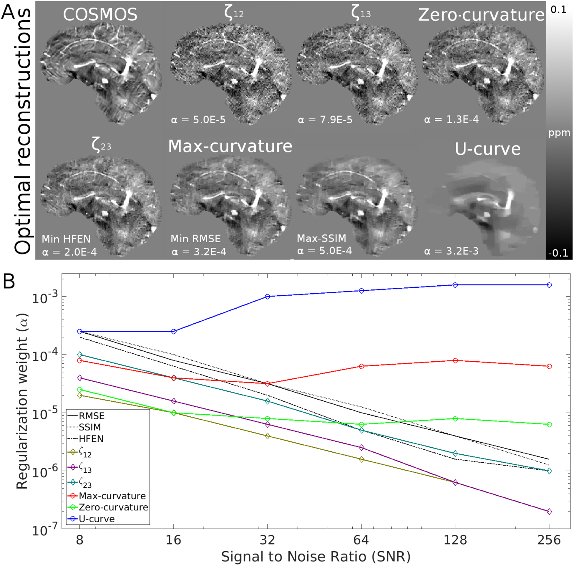
COSMOS-based simulation. (A) shows the optimal reconstructions and regularizations weights (α) using the Frequency, L-curve and U-curve analysis, along with the ground-truth. Also represented here are the best scoring HFEN, RMSE and SSIM results. (B) shows the evolution of the optimal regularization weights for each method and metric as function of the SNR.

This correlation between L-curve predictors and the quality metrics, however, do not remain the same for different SNR settings (Figure 3B). The optimal values predicted by the L-curve analysis seem to fail to account for the difference in SNR, yielding very similar results in all scenarios (mostly, over-regularizing for high SNR). Frequency-based estimations, on the other hand, present a strong dependency of the SNR, with ζ₂₃ having a good correlation with the HFEN metric. Results for the SNR=128 simulation are displayed in Supporting Information Figures S3 and S4.

In vivo data

Whereas the QSM Challenge in vivo experiment represents a low SNR scenario for QSM, it is still larger than the SNR=40 analytic experiment shown earlier. Results are presented in Figure 4 and Figure 5. While all L-curve based weights seem to over-regularize the solutions, the frequency analysis yielded more visually appealing results. Tissue contrast of the ζ₂₃ solution is higher than L-curve based methods, although it shows minor noise amplification (under-regularization) and weak streaking artifacts are also evident.

Figure 4.

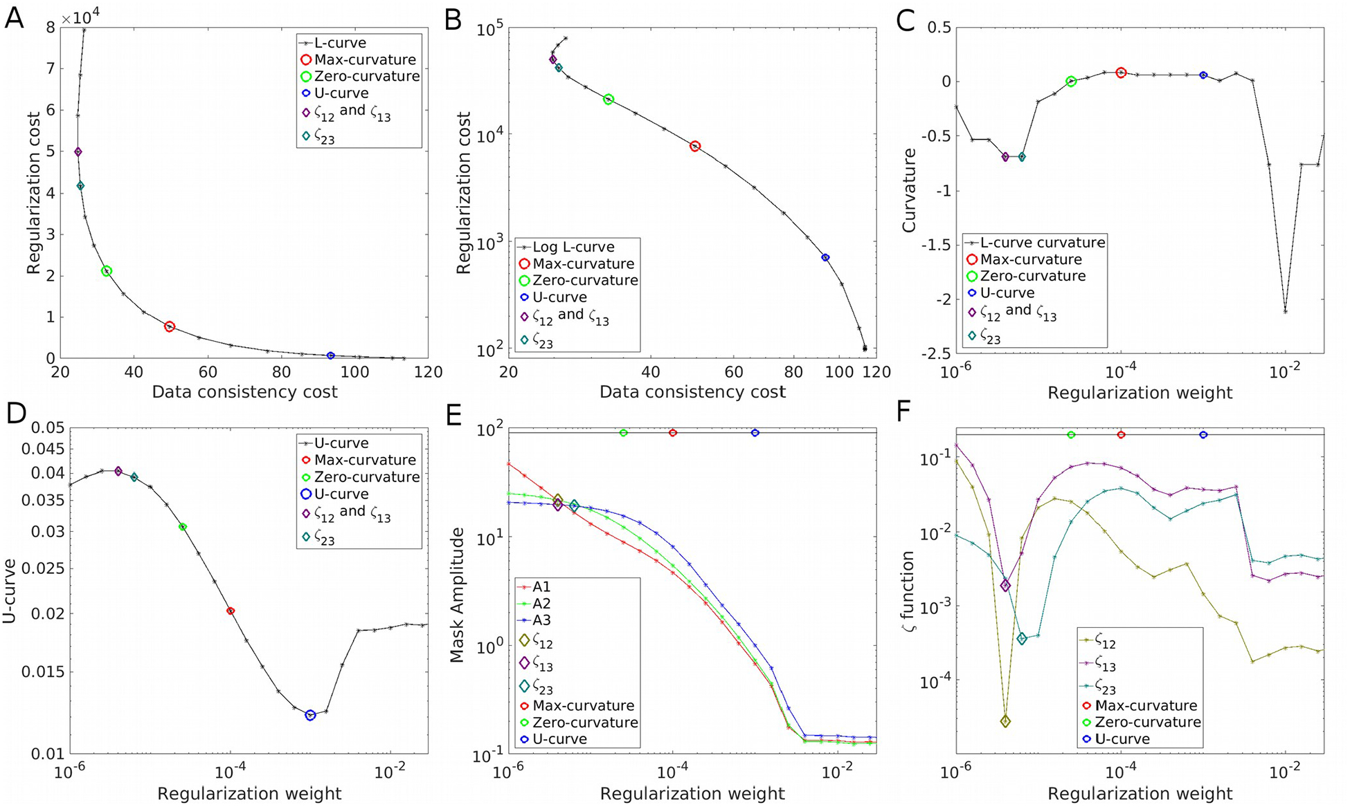
Parameter optimization strategies on the QSM Challenge in vivo data. The L-curve in linear (A) and logarithm (B) representations, with its curvature (C). The U-curve (D). Frequency analysis using the amplitude estimations A1, A2 and A3 (E) and the ζ cost functions (F).

Figure 5.

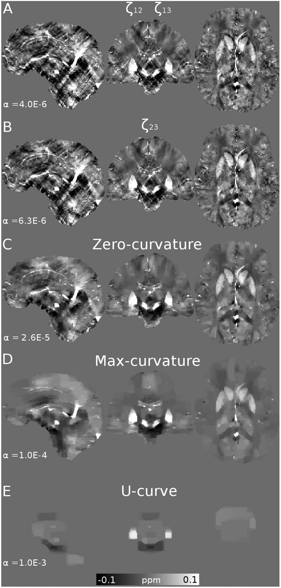
Optimal reconstructions and regularizations weights (α) of the QSM Challenge in vivo data, using the Frequency (A, B), L-curve (C, D) and U-curve analysis (E).

Reconstruction quality metrics with respect to COSMOS are provided for reference in the Supporting Information Table S1. As reported in Milovic et al³⁵, these metrics should not be considered as proper error metrics, since both COSMOS and χ₃₃ (STI) ground-truths incorporate anisotropic and micro-structural contributions that are not present in the single-orientation acquisition, creating significant discrepancies^35–37. This results in over-regularized reconstructions when using such metrics and ground-truth datasets for parameter optimization.

Additional in vivo results (presented in the Supporting Information Figures S5 to S8) confirm the findings by this in vivo experiment.

Figures 6 and 7 show the results of the L-curve, U-curve, and the frequency analysis. By using the amplitude estimators with the standard masks, ζ₂₃ cannot be assessed properly. The result is heavily over-regularized, with strong attenuations of all coefficients. This experiment shows a different behavior to those previously reported because of the highly anisotropic voxels. As shown in Figure 8, frequency coefficients close to the z-axis (parallel to the main field) contain more relevant information in medium and high frequencies. This is represented in the Power Spectrum as a region with higher local mean values, and more visible patterns. For this reason, masks were adjusted from the standard formulation (Figure 8A) to an alternative selection of regions of interest (Figure 8B and C). The new masks select regions of the frequency domain that are more homogeneous, with similar local mean values. By keeping the range of dipole kernel coefficients constant, but modifying the frequency range to target higher frequencies, our analysis is further degraded (Supporting Information Figures S9 and S10). Better results are achieved by keeping all masks in the same range of frequencies (Figure 8C). In this case, only positive dipole kernel values were selected, avoiding the XY plane (M₁ = 0<D<0.08, M₂ = 0.1<D<0.2 and M₃ = 0.22<D<0.32). The frequency range selected was 0.81 1/mm to 1.19 1/mm, to avoid selecting coefficients with too much structural information.

Figure 6.

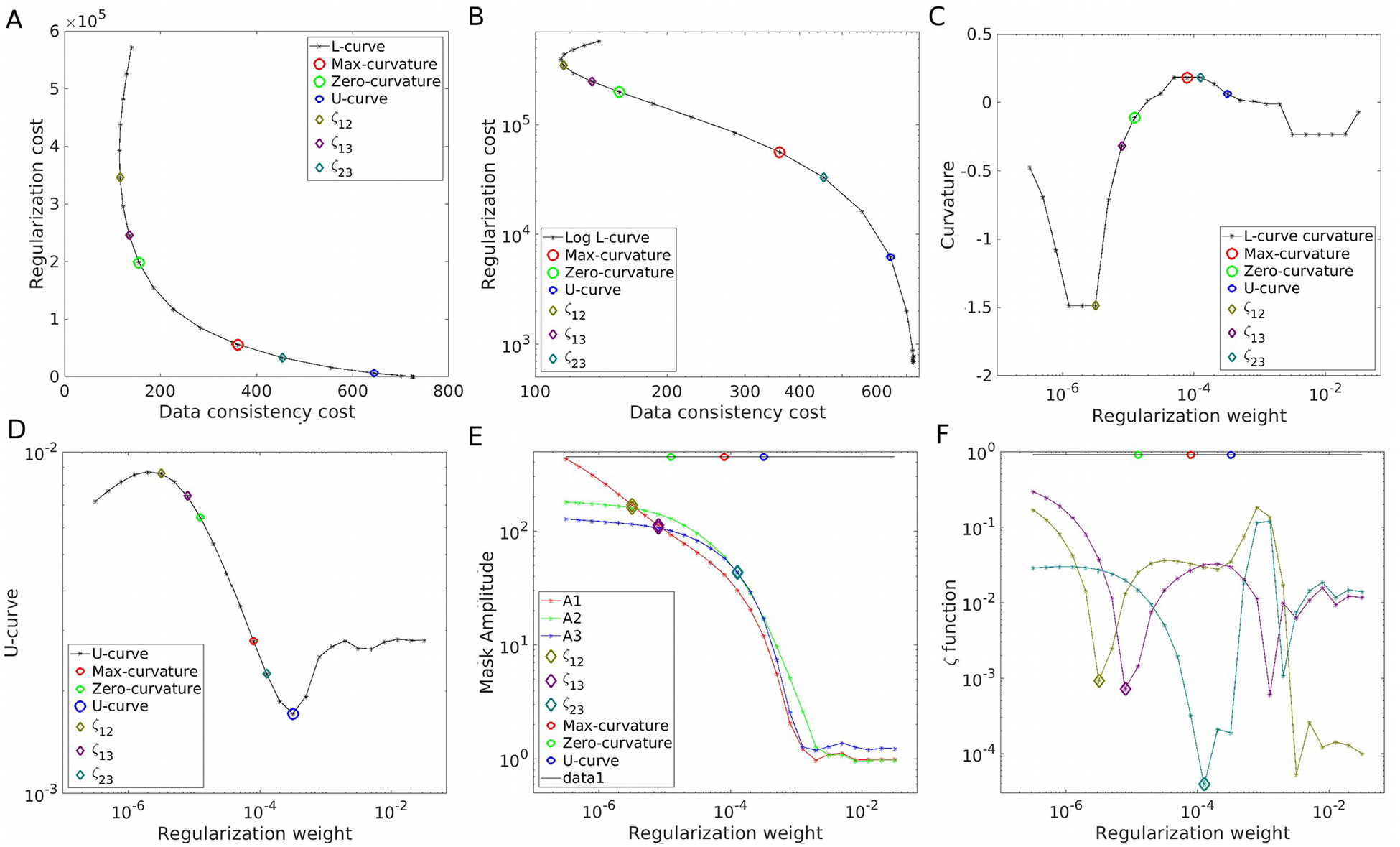
Parameter optimization strategies on the 7T Siemens in vivo data. The L-curve in linear (A) and logarithm (B) representations, with its curvature (C). The U-curve (D). Frequency analysis using the amplitude estimations A1, A2 and A3 (E) and the ζ cost functions (F).

Figure 7.

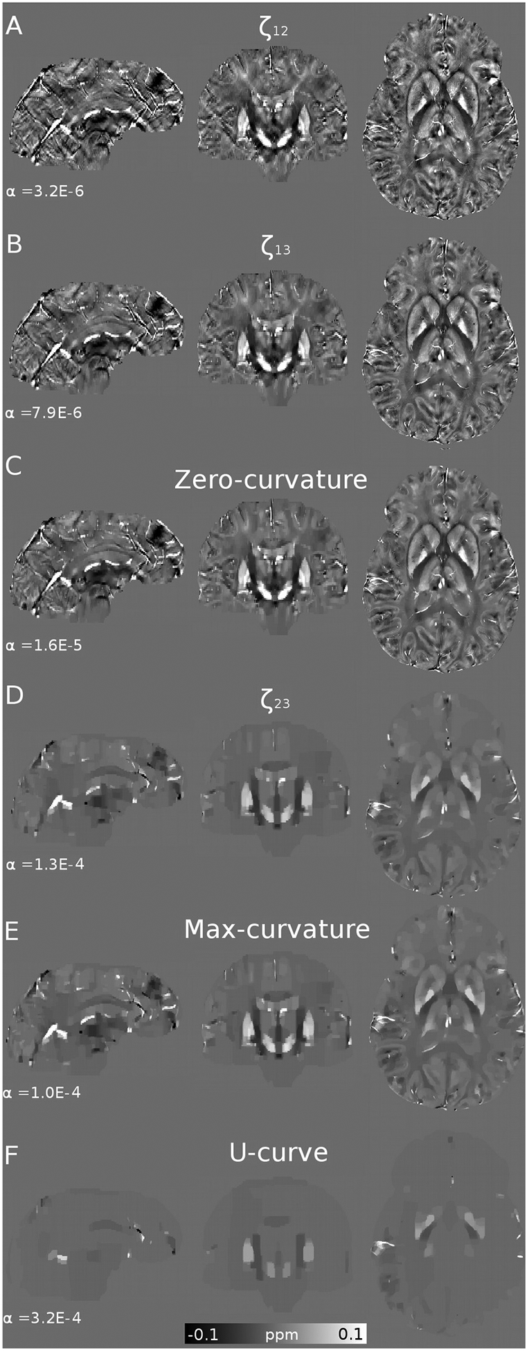
Optimal reconstructions and regularizations weights (α) of the 7T Siemens in vivo data, using the Frequency (A, B, E), L-curve (B, C) and U-curve analysis (D).

Figure 8.

Coronal and sagittal cuts for Fourier transform of the original ROIs masks (A), and arbitrary selection of frequency ranges and same dipole kernel coefficients (B), and the modified ROIs masks to account for the anisotropy and the uneven frequency distribution.

Results using this alternative masking procedure are shown in Figures 9 and 10. Now all the amplitude estimator curves intercept (Figure 9E), and the ζ functions show clear minimum values. Visually, now the results resemble those findings by previous experiments, with the ζ₂₃ based solution having more contrast and details than the Zero-curvature method (other methods with the same results as in Figure 7 are omitted).

Figure 9.

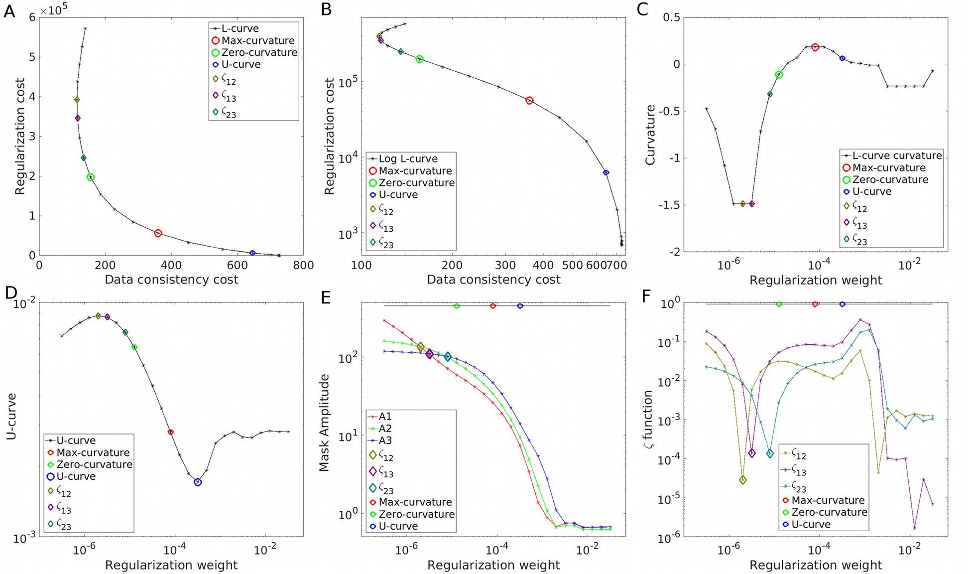
Parameter optimization strategies on the 7T Siemens in vivo data with modified ROIs. The L-curve in linear (A) and logarithm (B) representations, with its curvature (C). The U-curve (D). Frequency analysis using the amplitude estimations A1, A2 and A3 (E) and the ζ cost functions (F).

Figure 10.

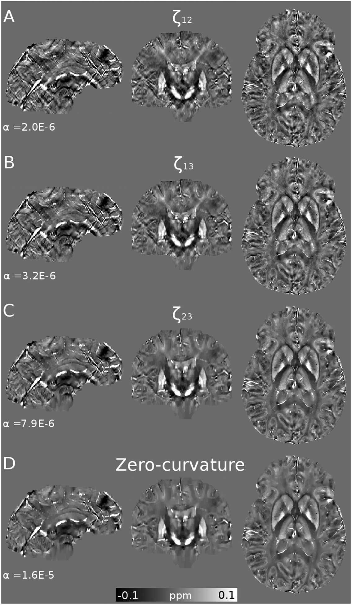
Optimal reconstructions and regularizations weights (α) of the 7T Siemens in vivo data with modified ROIs, using the Frequency (AC), and zero-curvature point of the L-curve (D).

Discussion

Here we presented two strategies to narrow down the search for an optimal regularization weight value in TV-based approaches for QSM, where the standard L-curve analysis is not reliable. The two approaches are: 1) searching for an inflection point in the log-log domain, and 2) analyzing the frequency components of the QSM reconstructions.

For the standard L-curve scheme, local curvature calculations, obtained by spline interpolation, often do not reflect the overall behavior and may be highly distorted by numerical errors. In addition, due to the different norms (L2-norm data fidelity and L1-norm regularizer) and domains (phase or complex signal domain vs gradient of susceptibilities) involved in the functional costs, the order of magnitude of each cost term differs significantly. This biases the calculation of the maximum curvature or the closest point to the origin. Changes in one term outweigh those in the other, and this is reflected in the curvature calculation. Furthermore, the L-curve may present wild oscillations far from the turn-off point, making an automatic/unsupervised search unreliable. Working on the logarithm domain prevents some of these problems, but the maximum curvature in such domain may not coincide with the one in the original domain. The inflection point in this curve seems to be a more reliable and robust starting point to search for an optimal regularization weight. As seen in our experiments, this point gives smaller weights than the maximum curvature criteria. While this point still usually yields over-regularized results, it may be used as an upper bound limit for visual optimization.

The second proposed strategy is based on the analysis of the amplitude of the frequency coefficients of the reconstructions. A proper solution must achieve a certain balance between all frequency coefficients where dipole kernel inversion does not amplify noise or create streaking artifacts, and the regularization term does not attenuate high-frequency terms, with over-smoothed results. To achieve this balance, we proposed to compare the mean amplitude of the frequency coefficients between two ROIs and select the regularization weight that equalizes them. Our results show that using ROIs that do not cover the magic angle produces more visually appealing results, with less streaking artifacts. In vivo experiments revealed that this optimization strategy may return regularization weights that are still too low to avoid the propagation of some streaking artifacts, especially those generated near the boundaries due to imperfect background filtration. In the presence of voxel asymmetries, the estimation of the frequency local amplitudes may be affected. Having significant structural information inside a mask may prevent its local mean to reach the same value as the local mean of another region, for a given set of regularization weights. Finding the minimum distance between the amplitude curves using the ζ function with the proposed masks (Eq. (8)) is still a good predictor for moderate asymmetries. In the presence of highly asymmetric voxels, the ROI mask should be modified (as shown in Figures 6–10). It was found that keeping all the ROI masks covering the same range of absolute frequencies (1/mm) is important to balance the amplitude measurements. Similar to our first proposed strategy, frequency equalization may serve to set a lower bound limit for a subsequent visual fine-tuning process. For a fully-automated (and standalone) approach, a correction factor may be used. Figure 3 suggests that due to the highly linear dependency between ζ₂₃ and RMSE and SSIM scores, a multiplicative factor between 1.5 and 2.0 should be used. Coincidentally, this gives results similar to those found by the Zero-curvature criteria in our in vivo experiments.

The proposed approaches were also compared to the U-curve analysis. However, the U-curve scheme failed to yield a reasonable result in all our experiments, producing heavily over-regularized results. This may be caused by an unbalance in the order of magnitude of the costs, due to the use of different norms and domains. Modifications to the U-curve method must be further investigated in the future to better address this issue when working with variational penalties (i.e. Total Variation or Total Generalized Variation). This may require working with logarithmic costs, or tailored weighting schemes.

One advantage of our frequency equalization strategy over the L-curve analysis is that this process does not require an exhaustive search to determine the optimal weights. To calculate the curvature at any point, the costs at two additional points are needed. To determine the balance between frequency coefficients only one result is needed. If the external ROI has larger amplitudes than the internal, then too large regularization weights are obtained. Smart search strategies may be developed, like a binary search or interpolation. This feature may allow our frequency equalization strategy to be implemented in a bilevel optimization¹⁰, or use it in an iteratively reweighted¹¹ mode to automatically achieve optimal results. Further experiments are needed to validate this. Another advantage of our method is that it seems to be more sensitive to changes in the SNR, as shown in Figure 1B. The ζ23 predictor seems to be more correlated with RMSE, SSIM, and HFEN for a wide range of noise levels, whereas the Zero-curvature method seems to work better in the 64–128 range. A scaling factor between 1.5 and 2.0 seemed to relate optimal RMSE reconstructions and ζ₂₃. Both ζ₂₃ and the Max-curvature methods seemed to be reliable for typical in vivo acquisitions. The preliminary examples presented here show that the Zero-curvature method is more robust against streaking or ghosting artifacts, but it may also suffer from sub-estimation and the loss of some fine structures due to over-regularization. Unfortunately, QSM is an ill-posed problem, prone to non-local artifacts, which may benefit from such over-regularization. A thorough study is needed to validate the robustness of these methods for quantitative studies, and the sensitivity to dipole-incompatible phase errors or background remnants. This validation study may also include multi-orientation acquisitions to assess the impact of the orientation of the tissues to the definition of the frequency masks.

Conclusions

We have developed two new regularization weight optimization strategies that yield more visually appealing and robust results than current user-independent methods. Jointly used, they may serve to set a range of possible alpha values, for manual (visual) optimization. Simulations suggest that the ζ₂₃ predictor may be used in a fully automatic algorithm, accounting with a multiplicative factor between 1.5 and 2.0 the difference between this function’s regularization weight and the one with optimal RMSE and SSIM scores. Such corrected regularization weights are well correlated with the Zero-curvature method for typical in vivo acquisitions. Regarding the computation expense of these calculations, the frequency equalization scheme may be used in more efficient schemes to automatically achieve visually appealing results without an exhaustive search of the optimal parameters. This includes the binary search and a smart selection of the evaluation points by using interpolations. Such a scheme may accelerate considerably the search of optimal regularization parameters.

Supplementary Material

supplementary

Supporting Information Figure S1. 3D representation of the ROIs used for the frequency analysis of susceptibility reconstructions. In red, M1: 0<=|D|<=0.085 at the magic angle. M2: 0.15<=|D|<=0.3 in green and M3: 0.35<=|D|<=0.6 in blue.

Supporting Information Figure S2. Optimal reconstructions and regularizations weights (α) of SNR=40 simulations, using the Frequency (A, B and D), L-curve (C, E) and U-curve analysis (G). Also represented here are the best scoring HFEN (D), RMSE (E) and SSIM (F) results.

Supporting Information Figure S3. Parameter optimization strategies on the COSMOS-brain simulations at SNR=128. The L-curve in linear (A) and logarithm (B) representations, with its curvature (C). The U-curve (D). Frequency analysis using the amplitude estimations A1, A2 and A3 (E) and the ζ cost functions (F).

Supporting Information Figure S4. Optimal reconstructions and regularizations weights (α) of SNR=128 simulations, using the Frequency (A, C), L-curve (E, F) and U-curve analysis (G). Also represented here are the best scoring HFEN (B), RMSE and SSIM (D) results.

Supporting Information Figure S5. Parameter optimization strategies on the 3T Siemens in vivo data. The L-curve in linear (A) and logarithm (B) representations, with its curvature (C). The U-curve (D). Frequency analysis using the amplitude estimations A1, A2 and A3 (E) and the ζ cost functions (F).

Supporting Information Figure S6. Optimal reconstructions and regularizations weights (α) of the 3T Siemens in vivo data, using the Frequency (A-C), L-curve (D, E) and U-curve analysis (F).

Supporting Information Figure S7. Parameter optimization strategies on the 3T Phillips in vivo data. The L-curve in linear (A) and logarithm (B) representations, with its curvature (C). The U-curve (D). Frequency analysis using the amplitude estimations A1, A2 and A3 (E) and the ζ cost functions (F).

Supporting Information Figure S8. Optimal reconstructions and regularizations weights (α) of 3T Phillips in vivo data, using the Frequency (A-C), L-curve (D, E) and U-curve analysis (F).

Supporting Information Figure S9. Parameter optimization strategies on the 37 Siemens in vivo data. The L-curve in linear (A) and logarithm (B) representations, with its curvature (C). The U-curve (D). Frequency analysis using the amplitude estimations A1, A2 and A3 (E) and the ζ cost functions (F) with masks defined in a relative frequency range.

Supporting Information Figure S10. Optimal reconstructions and regularizations weights (α) of 7T Siemens in vivo data., using the Frequency (A, B, and E), L-curve (B, C), and U-curve analysis (D).

Supporting Information Table S1 Global metric scores (RMSE, HFEN, and SSIM) for the proposed reconstructions using COSMOS as ground truth.

References

- 1.Haacke EM, Brown R, Thompson M, Venkatesan R. Magnetic Resonance Imaging: Physical Principles and Sequence Design.
- 2.Salomir R, De Senneville BD, Moonen CTW. A fast calculation method for magnetic field inhomogeneity due to an arbitrary distribution of bulk susceptibility. Concepts Magn Reson. 2003;19B(1):26–34. doi: 10.1002/cmr.b.10083 [DOI] [Google Scholar]
- 3.Marques JPP, Bowtell R. Application of a fourier-based method for rapid calculation of field inhomogeneity due to spatial variation of magnetic susceptibility. Concepts Magn Reson Part B Magn Reson Eng. 2005;25(1):65–78. doi: 10.1002/cmr.b.20034 [DOI] [Google Scholar]
- 4.Wharton S, Schäfer A, Bowtell R. Susceptibility mapping in the human brain using threshold-based k-space division. Magn Reson Med. 2010;63(5):1292–1304. doi: 10.1002/mrm.22334 [DOI] [PubMed] [Google Scholar]
- 5.Shmueli K, de Zwart J a, van Gelderen P, Li T-Q, Dodd SJ, Duyn JH. Magnetic susceptibility mapping of brain tissue in vivo using MRI phase data. Magn Reson Med. 2009;62(6):1510–1522. doi: 10.1002/mrm.22135 [DOI] [PMC free article] [PubMed] [Google Scholar]
- 6.Kee Y, Liu Z, Zhou L, et al. Quantitative Susceptibility Mapping (QSM) Algorithms: Mathematical Rationale and Computational Implementations. IEEE Trans Biomed Eng. 2017;64(11):2531–2545. doi: 10.1109/TBME.2017.2749298 [DOI] [PubMed] [Google Scholar]
- 7.Liu Z, Kee Y, Zhou D, Wang Y, Spincemaille P. Preconditioned total field inversion (TFI) method for quantitative susceptibility mapping. Magn Reson Med. 2017;78(1):303–315. doi: 10.1002/mrm.26331 [DOI] [PMC free article] [PubMed] [Google Scholar]
- 8.Liu C, Li W, Tong K a., Yeom KW, Kuzminski S. Susceptibility-weighted imaging and quantitative susceptibility mapping in the brain. J Magn Reson Imaging. 2014;00:n/a–n/a. doi: 10.1002/jmri.24768 [DOI] [PMC free article] [PubMed] [Google Scholar]
- 9.Weller DS, Ramani S, Nielsen JF, Fessler JA. Monte Carlo SURE-based parameter selection for parallel magnetic resonance imaging reconstruction. Magn Reson Med. 2014;71(5):1760–1770. doi: 10.1002/mrm.24840 [DOI] [PMC free article] [PubMed] [Google Scholar]
- 10.De los Reyes JC, Schönlieb CB, Valkonen T. Bilevel Parameter Learning for Higher-Order Total Variation Regularisation Models. J Math Imaging Vis. 2017;57(1):1–32. doi: 10.1007/s10851-016-0662-8 [DOI] [PMC free article] [PubMed] [Google Scholar]
- 11.Dong Y, Hintermüller M, Rincon-Camacho MM. Automated regularization parameter selection in multi-scale total variation models for image restoration. J Math … 2011:1–36. http://link.springer.com/article/10.1007/s10851-010-0248-9. Accessed August 22, 2014. [Google Scholar]
- 12.Hansen PC. The L-Curve and its Use in the Numerical Treatment of Inverse Problems. Comput Inverse Probl Electrocardiology, ed P Johnston, Adv Comput Bioeng. 2000;4:119–142. doi:10.1.1.33.6040 [Google Scholar]
- 13.Bilgic B, Fan AP, Polimeni JR, et al. Fast quantitative susceptibility mapping with L1-regularization and automatic parameter selection. Magn Reson Med. 2013;00. doi: 10.1002/mrm.25029 [DOI] [PMC free article] [PubMed] [Google Scholar]
- 14.Rudy Y, Ramanathan C, Ghanem R, Jia P. System and methods for noninvasive electrocardiographic imaging (ECGI) using generalized minimum residual (GMRes). US Pat No 7016719 . October 2006. https://patents.google.com/patent/US7016719B2/en.
- 15.Vogel CR. Non-convergence of the L-curve regularization parameter selection method. Inverse Probl. 1996;12(4):535–547. doi: 10.1088/0266-5611/12/4/013 [DOI] [Google Scholar]
- 16.Wei H, Dibb R, Zhou Y, et al. Streaking artifact reduction for quantitative susceptibility mapping of sources with large dynamic range. NMR Biomed. 2015;28(10):1294–1303. doi: 10.1002/nbm.3383 [DOI] [PMC free article] [PubMed] [Google Scholar]
- 17.Chamorro-Servent J, Dubois R, Coudière Y. Considering New Regularization Parameter-Choice Techniques for the Tikhonov Method to Improve the Accuracy of Electrocardiographic Imaging. Front Physiol. 2019;10:273. doi: 10.3389/fphys.2019.00273 [DOI] [PMC free article] [PubMed] [Google Scholar]
- 18.Wang Y, Liu T. Quantitative susceptibility mapping (QSM): Decoding MRI data for a tissue magnetic biomarker. Magn Reson Med. 2015;00(1):82–101. doi: 10.1002/mrm.25358 [DOI] [PMC free article] [PubMed] [Google Scholar]
- 19.Liu T, Wisnieff C, Lou M, Chen W, Spincemaille P, Wang Y. Nonlinear formulation of the magnetic field to source relationship for robust quantitative susceptibility mapping. Magn Reson Med. 2013;69(2):467–476. doi: 10.1002/mrm.24272 [DOI] [PubMed] [Google Scholar]
- 20.Milovic C, Bilgic B, Zhao B, Acosta-Cabronero J, Tejos C. Fast nonlinear susceptibility inversion with variational regularization. Magn Reson Med. 2018;80(2):814–821. doi: 10.1002/mrm.27073 [DOI] [PubMed] [Google Scholar]
- 21.Liu J, Liu T, de Rochefort L, Khalidov I, Prince MR, Wang Y. Quantitative susceptibility mapping by regulating the field to source inverse problem with a sparse prior derived from the Maxwell equation: validation and application to brain. Proceedings of the 18th Annual Meetting of ISMRM, Stockholm, Sweden, 2010. p 4996. [Google Scholar]
- 22.Bilgic B, Chatnuntawech I, Langkammer C, Setsompop K. Sparse methods for Quantitative Susceptibility Mapping In: Papadakis M, Goyal VK, Van De Ville D, eds. Wavelets and Sparsity XVI. Vol 9597 ; 2015:959711. doi: 10.1117/12.2188535 [DOI] [Google Scholar]
- 23.Kim TH and Haldar JP. Assessing MR image reconstruction quality using the fourier radial error spectrum plot. Proceedings 26th Annual Meeting International Society for Magnetic Resonance in Medicine Paris, France 2018:p0249 http://archive.ismrm.org/2018/0249.html [DOI] [PMC free article] [PubMed] [Google Scholar]
- 24.Diefenbach MN, Böhm C, Meineke J, Liu C, and Karampinos DC. One-Dimensional k-Space Metrics on Cone Surfaces for Quantitative Susceptibility Mapping. Proceedings 27th Annual Meeting International Society for Magnetic Resonance in Medicine Montreal, Canada 2019:p0322 https://index.mirasmart.com/ISMRM2019/PDFfiles/0322.html [Google Scholar]
- 25.Chamorro-Servent J, Aguirre J, Ripoll J, Vaquero JJ, Desco M. Feasibility of U-curve method to select the regularization parameter for fluorescence diffuse optical tomography in phantom and small animal studies. Opt Express. 2011;19(12):11490. doi: 10.1364/OE.19.011490 [DOI] [PubMed] [Google Scholar]
- 26.Chen M, Su H, Zhou Y, Cai C, Zhang D, Luo J. Automatic selection of regularization parameters for dynamic fluorescence molecular tomography: a comparison of L-curve and U-curve methods. Biomed Opt Express. 2016;7(12):5021–5041. doi: 10.1364/BOE.7.005021 [DOI] [PMC free article] [PubMed] [Google Scholar]
- 27.Milovic C, Bilgic B, Zhao B, Langkammer C, Tejos C, Acosta-Cabronero J. Weak-harmonic regularization for quantitative susceptibility mapping. Magn Reson Med. 2019;81(2):1399–1411. doi: 10.1002/mrm.27483 [DOI] [PubMed] [Google Scholar]
- 28.Liu T, Spincemaille P, De Rochefort L, Kressler B, Wang Y. Calculation of susceptibility through multiple orientation sampling (COSMOS): A method for conditioning the inverse problem from measured magnetic field map to susceptibility source image in MRI. Magn Reson Med. 2009;61:196–204. doi: 10.1002/mrm.21828 [DOI] [PubMed] [Google Scholar]
- 29.Langkammer C, Schweser F, Shmueli K, et al. Quantitative susceptibility mapping: Report from the 2016 reconstruction challenge. Magn Reson Med. 2018;79:1661–1673. doi: 10.1002/mrm.26830 [DOI] [PMC free article] [PubMed] [Google Scholar]
- 30.Bilgic B, Gagoski BA, Cauley SF, et al. Wave-CAIPI for highly accelerated 3D imaging. Magn Reson Med. 2015;73:2152–2162. doi: 10.1002/mrm.25347 [DOI] [PMC free article] [PubMed] [Google Scholar]
- 31.Wang Z, Bovik AC, Sheikh HR, Simoncelli EP. Image Quality Assessment: From Error Visibility to Structural Similarity. IEEE Trans Image Process. 2004;13:600–612. doi: 10.1109/TIP.2003.819861 [DOI] [PubMed] [Google Scholar]
- 32.Li W, Avram AV, Wu B, Xiao X, Liu C. Integrated Laplacian-based phase unwrapping and background phase removal for quantitative susceptibility mapping. NMR Biomed. 2014;27:219–227 [DOI] [PMC free article] [PubMed] [Google Scholar]
- 33.Li W, Wu B, Liu C. Quantitative susceptibility mapping of human brain reflects spatial variation in tissue composition. NeuroImage. 2011;55:1645–1656. [DOI] [PMC free article] [PubMed] [Google Scholar]
- 34.Ponomarenko N, Jin L, Ieremeiev O, Lukin V, Egiazarian K, Astola J, Vozel B, Chehdi K, Carli M, Battisti F, Kuo J. Image database TID2013: Peculiarities, results and perspectives. Signal Processing: Image Communication. 2015;30:57–77. doi: 10.1016/j.image.2014.10.009 [DOI] [Google Scholar]
- 35.Milovic C, Tejos C, Acosta-Cabronero J, Özbay P, Schwesser F, Marques JP, Irarrazaval P, Bilgic B, Langkammer C. The 2016 QSM Challenge: Lessons learned and considerations for a future challenge design; Magn Reson Med. 2020. doi: 10.1002/mrm.28185 [DOI] [PMC free article] [PubMed] [Google Scholar]
- 36.Wharton S and Bowtell R Effects of white matter microstructure on phase and susceptibility maps. Magn. Reson. Med, 2015;73: 1258–1269 [DOI] [PMC free article] [PubMed] [Google Scholar]
- 37.Lancione M, Tosetti M, Donatelli G, Cosottini M, Costagli M The impact of white matter fiber orientation in single-acquisition quantitative susceptibility mapping. NMR in Biomedicine. 2017; 30:e3798. [DOI] [PubMed] [Google Scholar]
Associated Data
This section collects any data citations, data availability statements, or supplementary materials included in this article.
Supplementary Materials