Determination of ethanol concentration in alcoholic beverages by direct analysis in real time mass spectrometry (DART-MS)

Abstract

Determination of the ethanol concentration in beverages remains an occasional request to forensic laboratories. While traditionally determined using headspace gas chromatography (HS-GC), this process involves lengthy run times and the need for specialized headspace sampling equipment for the GC system. The work presented here highlights a potential alternative to HS-GC analysis, using direct analysis in real time mass spectrometry (DART-MS). By incorporating a simple T-junction to the orifice of the mass spectrometer, analysis of the headspace of a beverage can be completed, resulting in measurement of the ethanol concentration in a matter of seconds with greater than 99% accuracy. This work presents the development of a method for ethanol quantitation as well as results from the analysis of both ethanol reference material standards and in-house created ethanol-containing solutions to evaluate the precision and accuracy of the technique. Analysis of ethanolic beverages via DART-MS is shown to be a rapid and reliable alternative to traditional analysis by HS-GC.

1. Introduction

In forensic analyses, the need occasionally arises to determine the concentration of ethanol in beverages to evaluate, among other things, whether a beverage has been tampered with. This analysis is typically completed by headspace gas chromatography (HS-GC) which can involve lengthy (on the order of minutes) run times as well as the need for additional equipment to complete headspace sampling instead of the more common liquid sampling [1,2]. This type of analysis is also completed in food safety analyses for investigative purposes, to determine if adulteration has occurred, or quality control purposes [3,4]. Techniques other than HS-GC have been demonstrated in literature - including Raman spectroscopy [5], Fourier transform infrared (FTIR) spectroscopy[6], spatially offset Raman spectroscopy [7], gas chromatography Fourier transform infrared (GC-IR) [8], and even Schlieren imaging [9].

Direct analysis in real time mass spectrometry (DART-MS) is an ambient ionization mass spectrometry technique that is witnessing increased use in forensic analyses [10]. DART-MS is appealing for many applications because it provides rapid analysis (on the order of seconds) of samples with minimal to no sample preparation. Previous work has shown the ability of DART-MS to analyze compounds such as drugs [11,12], explosives [13,14], lubricants [15], paints [16], and even woods [11]. Studies have also been completed utilizing DART-MS to analyze beverages for qualitative purposes to identify compounds of interest such as caffeine [17], phthalates [18], and gamma hydro-xybutyric acid (GHB) [19]. While the compounds of interest analyzed by DART-MS are normally higher in molecular weight than ethanol, recent work has highlighted the ability of this tool to detect low molecular weight adulterants, such as ammonia, bleach, methanol, and butanol in beverages [20]. Detection of these compounds, especially methanol, and others, such as iso-amyl alcohol, are crucial for adulteration detection [4].

This study builds upon previous work in the qualitative identification of low molecular weight compounds by DART-MS by extending to quantitative measurements of ethanol concentration in beverages. Utilizing a simple modification to the DART-MS interface to collect headspace vapors into the DART gas stream, a method for determining the ethanol concentration was created. This method was then used to evaluate whether quantitative information could be obtained with samples of known ethanol concentrations. The ability to re-analyze samples was also evaluated. The method described herein represents a viable alternative to ethanol quantitation in place of HS-GC analysis.

2. Materials & methods

2.1. Materials

Ethanol, isopropanol (IPA), and water were purchased from Sigma-Aldrich (St. Louis, MO, USA) as Chromasolv-grade reagents. Ethanol reference materials (ERMs) - beverages with analytically certified ethanol concentrations - were purchased from LGC Standards (Bury, UK) and included: Lager BA005a, Wine BA003a, and Brandy BA006a. Common beverages for creating mixed drinks (cola, pineapple juice, orange juice, and fruit punch) were used to create in-house ethanol-containing solutions.

2.2. Sample preparation

It is important to note that the volume compression of ethanol-water mixtures [21,22] was not taken into consideration for the calculations of the final volumes of all solutions prepared. This non-additive property of volumetric mixtures of ethanol and water would have a greater impact on the mid-range ethanol concentrations (10% v/v to 50% v/v) resulting in the actual ethanol concentration to be slightly higher than calculated in this range. For method development and parametric studies, a 50% (v/v) mixture of ethanol and water was prepared by adding equivalent volumes of each liquid. The solutions for the limits of detection determinations were made as 1:9 serial dilutions from pure ethanol. For calibration, solutions of ethanol and water were prepared gravimetrically to obtain a 9-point calibration curve. Specific gravities of water and ethanol were then used to convert the gravimetric values to percent by volume; values which ranged from 0% v/v ethanol to 100% v/v ethanol. ERMs were used as received. The additional non-alcoholic beverages were spiked with ethanol to obtain a range of ethanol concentrations by pipetting a known volume of ethanol into a known volume of the beverage. Once the appropriate ethanol concentration was prepared, 1 mL aliquots of the sample were pipetted into 2 mL amber vials and 0.25 mL of isopropanol (used as the internal standard) was added via pipette (to bring the total volume to1.25 mL). Vials were then vortexed for 15 s. The samples were left undisturbed for at least one hour, and as long as overnight, to allow for headspace to equilibrate. The stock calibration solutions and the spiked mixed beverages were stored at 4 °C between analyses and allowed to warm to room temperature (approximately 23 °C) before aliquots were removed. The aliquots were removed from the stock containers and spiked with the internal standard to allow for ethanol and isopropanol to equilibrate in the headspace of the sampling vials only as needed for analysis, unless otherwise stated.

2.3. Instrumentation

Samples were analyzed using a DART-MS with an in-house built headspace configuration, a schematic of which is shown in Fig. 1. The mass spectrometer, a JEOL JMS-T100LP (JEOL USA, Peabody, MA, USA), was coupled with a Vapur® interface (IonSense, Saugus, MA, USA). To direct the pull of headspace of the sample into the Vapur interface, the ceramic tube of the Vapur interface was shortened to 30 mm and a Swagelok (Solon, OH, USA) T-junction was fitted to the end of the ceramic tube, which allowed uninterrupted flow of the DART gas while also allowing for the placement of the 2.0 mL glass vial directly underneath. Placement of the vial directly under the junction allowed for an approximately 2 mm air gap between the vial and junction. This configuration promoted the entrainment of the headspace from the vial into the DART gas stream. Analysis was completed by placing uncapped vials under the T-junction and allowing the headspace to be sampled for 8 s to 10 s. Helium (99.999% purity) was used as the DART source gas for all analyses. Unless otherwise stated, relevant instrument parameters included a DART exit grid voltage of 150 V, a 350 °C DART gas temperature, and a Vapur flow rate of 3.5 L min⁻¹. Mass spectrometer settings included: operation in positive ionization mode, a 110 °C Orifice 1 temperature, 100 V ion guide voltage, 25 V orifice 1 voltage, 20 V ring lens voltage, 5 V orifice 2 voltage, 2300 V detector voltage, and a mass scan range of m/z 20 to m/z 150 at0.25 s scan⁻¹. Polyethylene glycol 600 (PEG) was used for mass calibration.

Fig. 1.

Schematic of the DART-MS modification.

Ethanol quantitation was accomplished by integrating the peak areas of extracted ion chronographs of m/z 47 ([Ethanol + H]⁺) and m/z 61 ([IPA + H]⁺) using MassCenterMain software. Integration was completed using the integrate function of the software. The ratio of the peak areas (m/z 47: m/z 61) was then compared to a 9-point calibration curve to obtain the concentration of ethanol in the solution. The ethanol dimer peak of m/z 93 ([2 Ethanol + H]⁺) and the ethanol-IPA complex peak of m/z 107 ([Ethanol + IPA + H]⁺) were also monitored but were ultimately not used for quantitation.

2.4. Parametric studies

For the optimization of DART gas stream temperature, DART exit grid voltage, and Vapur flow rate a 300 V ion guide voltage and 20 V orifice 1 voltage was used. A 20 V orifice 1 voltage was used for the optimization of the ion guide voltage. A 100 V ion guide voltage was used for the optimization of the Orifice 1 voltage.

2.5. Analysis of ethanol containing beverages

For the analysis of ethanol containing beverages, identical settings as above were used except for a 100 V ion guide voltage, and a 30 V orifice 1 voltage.

3. Results & discussion

3.1. Method optimization & representative spectra

Development of a DART-MS method for the quantitation of ethanol involved optimizing the instrument for a compound that is traditionally viewed as the solvent molecule. Because of the high volatility and low molecular weight of ethanol, it was unknown whether an optimal DART-MS method would be significantly different than those used to analyze other common compounds. To identify optimal operation settings, several variables were examined using parametric studies and included: DART gas stream temperature, DART exit grid voltage, Vapur flow rate, ion guide voltage, and orifice 1 voltage. For the optimization studies, the signals of the ethanol monomer, isopropanol monomer, ethanol dimer, and ethanol-isopropanol complex, were monitored and the peak areas of those signals were plotted. The goal of these studies was to maximize the response of the monomer species. Each parameter was optimized individually with the remaining parameters held constant, as described previously. Four or five replicate measurements were made for all data points. The results of the optimization studies are presented in Fig. 2. For this work a 50% (v/v) ethanol and water mixture was used.

Fig. 2.

Average integrated peak areas of the ethanol monomer (m/z 47, blue circle), ethanol dimer (m/z 93, blue diamond), isopropanol monomer (m/z 61, orange circle) and ethanol-isopropanol complex (m/z 107, orange diamond) for the parametric study of Vapur flow rate (A.), DART gas stream temperature (B.), mass spectrometer ion guide voltage (C.), and mass spectrometer orifice 1 voltage (D.). The secondary axes in (A.) and (C.) correspond to the peak area for the isopropanol monomer (m/z 61) while the primary axes correspond to the peak areas for the remaining m/z values. Error bars represent the standard deviation of the four to five replicate measurements.

The most influential parameter tested was Vapur flow rate, which was examined across the range of 2.5 L min⁻¹ to 5.0 L min⁻¹. The Vapur flow rate controls the amount of analyte vapor that is pulled through the Swagelok and towards the mass spectrometer. As shown in Fig. 2A, an optimal flow rate of approximately 3.5 L min⁻¹ was observed for the monomer species, with a substantial decrease in signal being observed at higher flow rates. As the Vapur flow rates increase, which cause air to be pulled through the T-junction more rapidly, the resonance time of the analyte molecules within the T-junction decreases, lowering the probability of ionization. Sample dilution, due to increased air being mixed in with analyte vapor may also cause lower signal. Quantifying this loss in sensitivity with respective to increasing Vapur flow rate is the focus on ongoing work. Conversely, at lower Vapur flow rates, where some decrease in analyte signal was observed, there may be insufficient flow to entrain the headspace into the DART gas stream as the flow rate is lower than the flow rate of the DART source gas itself. Interestingly, flow rates less than 3.5 L min⁻¹ had minimal impact on the dimer and complex species, though substantial declines in monomer signals were observed.

DART gas stream temperature (Fig. 2B) and DART exit grid voltage (not pictured) had limited influence on the signal of both ethanol and isopropanol. Since both ethanol and isopropanol are volatile, and the DART gas was not being used to desorb the sample, varying the gas stream temperature had little effect. Maintaining a gas stream temperature above ambient temperature, however, should be utilized to prevent condensation of the analyte or the beverage vapors onto the walls of Swagelok and/or Vapur interface. No trend was observed in ethanol or isopropanol signal as a function of exit grid voltage.

The ion guide voltage, which is used as a low mass filter for the mass spectrometer, was also examined. For the mass spectrometer used in this work, the ion guide voltage corresponds to roughly a factor of ten greater than the low mass cutoff (i.e., an ion guide voltage of 200 V will allow ions of m/z 20 or greater through). As expected, the monomer species, which are at lower masses, are greatly influenced by increasing the ion guide voltage (Fig. 2C), while the dimer species showed little effect from an increasing ion guide voltage. Voltages in this range (less than 400 V), are traditionally not used for analysis of common compounds, but are necessary to obtain responses from the monomer species for this application.

The final component examined was the orifice 1 voltage on the mass spectrometer, which controls the extent of in-source collisionally induced dissociation (CID) that occurs. For the analysis of high volatility compounds, where dimerization and clustering of analytes is common, an appropriate orifice 1 voltage is crucial for minimization of the dimer species. As shown in Fig. 2D, dimerization can be minimized at a relatively low orifice 1 voltage of 25 V, which also corresponds to the maximum for the monomer ethanol and isopropanol species.

From these studies, a method for analysis was developed which included a Vapur flow rate of 3.5 L min⁻¹, a DART gas stream temperature of 350 °C, a DART exit grid voltage of 150 V, a mass spectrometer ion guide voltage of 100 V, and an orifice 1 voltage of 25 V. This method was used for all further studies. A representative mass spectrum of the ethanol isopropanol mixture under these conditions is shown in Fig. 3. The spectrum is dominated by the protonated ethanol and isopropanol molecules (at m/z 47 and m/z 61, respectively) as well as a background CH₃CO peak at m/z 43. Small peaks for the ethanol dimer (m/z 93) and the ethanol isopropanol complex (m/z 107) are also observed.

Fig. 3.

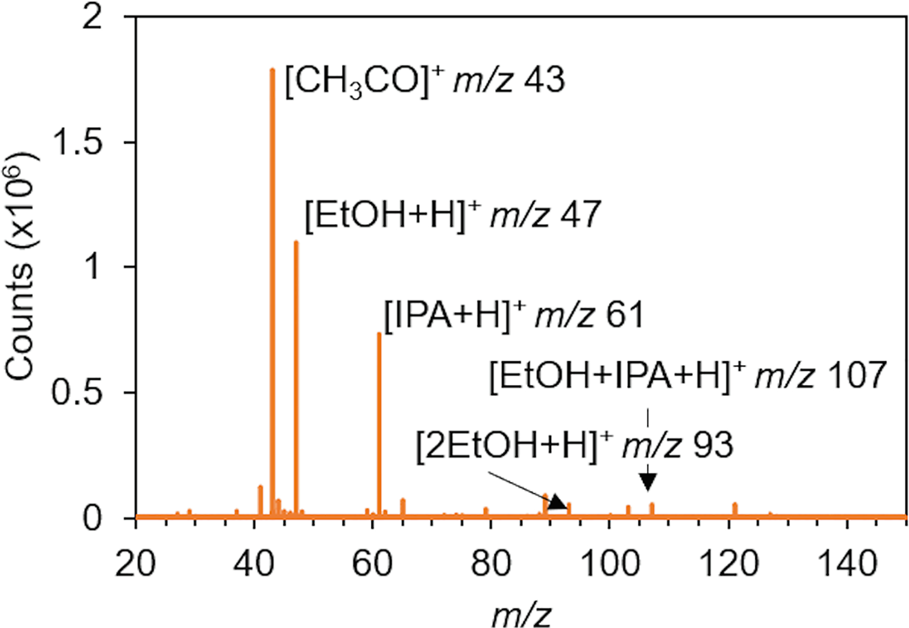
Representative mass spectrum of a 50% v/v ethanol and water mixture with isopropanol internal standard. Ethanol is abbreviated EtOH while isopropanol is abbreviated IPA.

3.2. Quantitation & limits of detection

Once an optimal method was established, efforts were made to identify the limit of detection (LOD) of ethanol in water mixtures. Calculation of LOD was completed using the ASTM E2677 method [23], which provides a 90% confidence for the LOD. To accomplish this, ten replicates of samples at 0% v/v, 0.1% v/v, 1.0% v/v, and 10.0% v/v were analyzed. Using the ASTM E2677 LOD calculator [24], an LOD₉₀ of 0.15% v/v ethanol in water was calculated.

Additional studies were completed to evaluate the ability to quantitate ethanol concentrations. Using a series of ethanol solutions from 0% v/v to 100% v/v, a linear response with a R² value of greater than0.997 (Fig. 4) was obtained. A y-intercept very close to zero was also observed, indicating the absence of any significant background at m/z 47 for ethanol. Deviation from the regression line was more evident in the mid-range ethanol concentrations (10% v/v to 50% v/v). This slight deviation is likely caused by the volume compression of ethanol–water mixtures [21,22] which would cause a greater number of ethanol molecules to be transferred in the 1 mL aliquot than if the pure liquid (water or ethanol) were transferred. The volume compression effect of the ethanol-water mixture was not accounted for in these curves. Additional aliquots from the same calibration curve were re-analyzed one week and up to 2 weeks after preparation to see if the calibration curve could be reused. It should be noted, however, that the response was different for the different analysis days. This may be a function of laboratory environmental conditions (i.e., temperature or humidity) and suggests the need for the calibration curve (or an abbreviation thereof) to be sampled during the same time that the unknowns are analyzed.

Fig. 4.

Calibration curves from the initial time taken (blue circle), one week after creation (green diamond), and a new calibration curve made six months after initial analysis (purple triangle). Uncertainties represent the standard deviation of ten replicate measurements.

3.3. Analysis of ethanol containing beverages

To evaluate the applicability of this method to quantitate unknowns, three ERMs, beverages with analytically certified ethanol concentrations, were tested. These ERMs were chosen to span the range of ethanol concentrations and included lager (reported concentration of 5% v/v), wine (15% v/v), and brandy (40% v/v). Samples were spiked with isopropanol as the internal standard and at least ten replicates were analyzed. The ratio of ethanol to isopropanol was then fitted to up to three different calibration curve windows (0% to 10% v/v, 0% to 50% v/v, and 0% to 100% v/v), when applicable, to determine if there was any effect from the range of the curve that was used due to the volume compression of the mid-range concentrations. Table 1 shows the average measured ethanol concentration of the ERMs using each of the three calibration curves. For the lowest curve, only the lager was quantitated as it was the only standard within the 0% v/v to 10% v/v range. In all instances, the calculated concentrations fell within 1% v/v of the documented concentrations, and the relative standard deviation of replicate measurements was below 15%, with higher relative variability observed for the low ethanol concentration lager. Additionally, there did not appear to be a dependence on the calibration curve range with respect to accuracy of the measurement, indicating that any calibration curve would be suitable for the measurement provided the unknown concentration fell within that range and that the volume compression could be considered negligible for this type of analysis. Deviations from the reported concentration may be due to variations in the calibration curve or due to differences caused by the process used to certify the ethanol concentration (distillation followed by measurement of the apparent density in air by pycnometry at 20 °C and compared to the “Laboratory Alcohol Table’ Reference RDC80/267/04). This study also highlighted that the presence of complex matrices did not affect the ability to quantitate the solution even though aqueous calibrants were used. A representative mass spectrum of the wine ERM is presented in Fig. 5A.

Table 1.

Measured ethanol concentrations for the three ERMs examined. The concentrations using different calibration curves are presented. Documented ethanol concentrations were 5% v/v, 15% v/v, and 40% v/v for the lager, wine and brandy respectively. The right three columns show the measured ethanol concentrations 6 months after making the first set of measurements. Uncertainties represent the standard deviation of ten replicate measurements.

Cal Curve Range (% v/v)	Measured Ethanol Concentration (% v/v)			Repeat Measurement After 6 Months (% v/v)
	Lager	Wine	Brandy	Lager	Wine	Brandy
0% to 10%	5.31 ( ± 0.67)	N/A	N/A	5.30 ( ± 0.04)	N/A	N/A
0% to 50%	5.24 ( ± 0.68)	14.89 ( ± 1.92)	40.13 ( ± 1.55)	5.25 ( ± 0.04)	15.32 ( ± 0.05)	41.69 ( ± 0.07)
0% to 100%	5.05 ( ± 0.78)	14.46 ( ± 0.80)	40.29 ( ± 3.80)	5.51 ( ± 0.30)	15.11 ( ± 0.03)	40.28 ( ± 0.68)

Fig. 5.

Representative mass spectra of the wine ERM (A.) and a 25% v/v solution of ethanol in cola (B.). The peak for the ethanol monomer is highlighted in orange while the peak for the isopropanol monomer is highlighted in grey.

Cases in a forensic laboratory may sit for some time before analysis, therefore repeat measurements of the same ERMs were made six months after the initial set of measurements to establish whether the results could be reproduced. For these samples a new calibration curve was created, and a new 1 mL aliquot was removed from the original ERM solutions. As shown in Table 1, results can be replicated even after a six-month window. Deviation from the reported ERM value was slightly higher for the 6-month-old samples than the freshly analyzed samples and may be attributable to the six-month storage period in the refrigerator.

To expand the investigation into matrix effects beyond the three ERMs, ethanol was spiked in four common mixing beverages (cola, pineapple juice, orange juice, and fruit punch) at four different concentrations (5% v/v, 10% v/v, 25% v/v, and 50% v/v). Ethanol was added volumetrically and 1 mL aliquots of the mixed solutions were placed in 2.0 mL amber vials and spiked with isopropanol internal standard. Ten replicates of each sample were analyzed, and the ethanol concentration calculated using a 0% v/v to 50% v/v calibration curve. The measured concentrations can be found in Table 2. Much like the ERMs, the measured ethanol concentration fell largely within ± 1% v/v of the prepared concentration. The standard deviation of the replicate measurements increased with ethanol concentration, though the relative standard deviation remained relatively constant, around 10%.

Table 2.

Measured ethanol concentrations for the in-house created mixed beverages, using a 0% v/v to 50% v/v calibration curve. Uncertainties represent the standard deviation of ten replicate measurements.

Nominal Ethanol Concentration (% v/v)	Measured Ethanol Concentration (% v/v)
	Cola	Pineapple Juice	Orange Juice	Fruit Punch
5%	5.03 ( ± 0.20)	4.81 ( ± 0.27)	5.07 ( ± 0.25)	4.88 ( ± 0.11)
10%	9.40 ( ± 0.76)	9.12 ( ± 1.17)	9.40 ( ± 0.84)	9.01 ( ± 0.83)
25%	23.49 ( ± 2.77)	22.17 ( ± 1.94)	23.32 ( ± 1.04)	26.89 ( ± 1.50)
50%	49.94 ( ± 2.12)	49.81 ( ± 4.73)	48.20 ( ± 4.38)	52.66 ( ± 1.42)

3.4. Ability to re-sample

The final component of the study investigated whether re-sampling of vials was possible to see if changes in the headspace of the sample occurred with repeat sampling. To investigate this, aqueous solutions containing 5% v/v and 50% v/v ethanol by volume were created volumetrically and the solutions were then split into 18 individual vials and spiked with isopropanol as an internal standard. Five of the vials were uncapped, sampled, and capped at each timepoint over the course of the 24-hour study while the remaining vials were sampled at only one of the 12 timepoints. The timepoints for resampling were: 0.5 h, 1 h, 1.5 h, 2 h, 2.5 h, 3 h, 3.5 h, 4 h, 4.5 h, 5 h, 5.5 h, and 24 h. The ethanol concentration of the single sample vial and the average of the resampled vials were then calculated.

The results of re-sampling study, shown in Fig. 6, show starkly different trends for the 5% v/v solution and the 50% v/v solution though both show changes in the headspace do occur with repeat analysis. For the 5% v/v solution, where ethanol was at a lower concentration than the isopropanol internal standard, the re-sampled vials trended lower than the actual initial concentration. This is likely due to an increasing fraction of isopropanol in the headspace of the vial which pushes the calculated ethanol concentration lower. When the ethanol concentration exceeds the isopropanol concentration, as was the case for the 50% v/v ethanol solution, the calculated concentration trends significantly higher than the initial concentration, likely due to the decreasing fraction of isopropanol in the headspace. In both instances, the number of data points outside the 2σ range (red dotted lines) was higher for the re-sampled vials than the single sample vial, indicating that repeat analysis of the same vial should be avoided in order to obtain the most accurate ethanol concentration.

Fig. 6.

Results of re-sampling study for the 5% v/v ethanol solution (A.) and the 50% v/v ethanol solution (B.). Blue circles indicate the new sample analyzed during that timepoint while the orange triangles represent the five re-sampled vials. Error bars represent the standard deviation of five replicate measurements. The red line represents the average calculated ethanol concentration for all the vials sampled only once. The dotted red lines indicate the ± 2 standard deviation lines of that sample set.

4. Conclusions

DART-MS represents a promising new technique for the quantitation of ethanol in beverages. Rapid determination of ethanol concentration in beverages can be achieved in a matter of seconds. Quantitation of ERMs with known ethanol concentrations provided measurements within ± 1% v/v, and accurate measurements were also shown in several other beverage matrices at varying concentrations. Some care, however, needs to be taken with this type of analysis as laboratory conditions may affect the response, leading for the need of the calibration curve, or a subset thereof, to ideally be run at the same time as the unknown samples. Repeat analysis of the same sample over time is also not recommended as the regeneration of the headspace will lead to differences in ethanol concentration - skewing higher at larger ethanol concentrations and lower at smaller ethanol concentrations. This technique provides a unique compliment or replacement to current tools such as HS-GC. Future work is focused on expanding the detection and quantitation capabilities of this technique to include other compounds that may be present in adulterated beverages, such as methanol, iso-amyl alcohol, and ethyl acetate butanol.

5. Disclaimer

Certain commercial products are identified in order to adequately specify the procedure; this does not imply endorsement or recommendation by NIST, nor does it imply that such products are necessarily the best available for the purpose.

HIGHLIGHTS.

• Quantitation of ethanol by DART-MS is possible in seconds.

• 0.15% v/v limit of detection possible.

• Simple modification allows entrainment of headspace.

• Minimal to no interference by beverage matrix.

• Re-sampling of the same sample if difficult.

• TRL Level: 3.

References

- [1].Kobilinsky L (Ed.), Forensic Chemistry Handbook, John Wiley & Sons, 2012. [Google Scholar]
- [2].Jung A, Jung H, Auwärter V, Pollak S, Farr AM, Hecser L, Schiopu A, Volatile congeners in alcoholic beverages: analysis and forensic significance, in: 2010. 10.4323/rjlm.2010.265. [DOI]
- [3].Wang M-L, Wang J-T, Choong Y-M, Simultaneous quantification of methanol and ethanol in alcoholic beverage using a rapid gas chromatographic method coupling with dual internal standards, Food Chem. 86 (2004) 609–615, 10.1016/j.foodchem.2003.10.029. [DOI] [Google Scholar]
- [4].Arslan MM, Zeren C, Aydin Z, Akcan R, Dokuyucu R, Keten A, Cekin N, Analysis of methanol and its derivatives in illegally produced alcoholic beverages,J. Foren. Legal Med 33 (2017) 56–60, 10.1016/j.jflm.2015.04.005. [DOI] [PubMed] [Google Scholar]
- [5].Boyaci IH, Genis HE, Guven B, Tamer U, Alper N, A novel method for quantification of ethanol and methanol in distilled alcoholic beverages using Raman spectroscopy, J. Raman Spectrosc 43 (2012) 1171–1176, 10.1002/jrs.3159. [DOI] [Google Scholar]
- [6].Debebe A, Redi-Abshiro M, Chandravanshi BS, Non-destructive determination of ethanol levels in fermented alcoholic beverages using Fourier transform mid-infrared spectroscopy, Chem. Central J 11 (2017) 27, 10.1186/s13065-017-0257-5. [DOI] [PMC free article] [PubMed] [Google Scholar]
- [7].Ellis DI, Eccles R, Xu Y, Griffen J, Muhamadali H, Matousek P, Goodall I,Goodacre R, Through-container, extremely low concentration detection of multiple chemical markers of counterfeit alcohol using a handheld SORS device | Scientific Reports, Sci. Rep 7 (2017), 10.1038/s41598-017-12263-0. [DOI] [PMC free article] [PubMed] [Google Scholar]
- [8].Sharma K, Sharma SP, Lahiri S, Novel Method for Identification and Quantification of Methanol and Ethanol in Alcoholic Beverages by Gas Chromatography-Fourier Transform Infrared Spectroscopy and Horizontal Attenuated Total Reflectance Fourier Transform Infrared Spectroscopy, (2009). https://www.ingentaconnect.com/content/aoac/jaoac/2009/00000092/00000002/art00020 (accessed June 17, 2019). [PubMed] [Google Scholar]
- [9].Vidigal SSMP, Rangel AOSS, A reagentless flow injection system for the quantification of ethanol in beverages based on the schlieren effect measurement, Microchem. J 121 (2015) 107–111, 10.1016/j.microc.2015.02.006. [DOI] [Google Scholar]
- [10].Pavlovich MJ, Musselman B, Hall AB, Direct analysis in real time—Mass spectrometry (DART-MS) in forensic and security applications, Mass Spec Rev. (2016), 10.1002/mas.21509. [DOI] [PubMed] [Google Scholar]
- [11].Lesiak AD, Shepard JR, Recent advances in forensic drug analysis by DART-MS, Bioanalysis 6 (2014) 819–842, 10.4155/bio.14.31. [DOI] [PubMed] [Google Scholar]
- [12].Sisco E, Verkouteren J, Staymates J, Lawrence J, Rapid detection of fentanyl, fentanyl analogues, and opioids for on-site or laboratory based drug seizure screening using thermal desorption DART-MS and ion mobility spectrometry, Foren. Chem 4 (2017) 108–115, 10.1016/j.forc.2017.04.001. [DOI] [PMC free article] [PubMed] [Google Scholar]
- [13].Sisco E, Dake J, Bridge C, Screening for trace explosives by AccuTOFTM-DART®: an in-depth validation study, Forensic Sci. Int 232 (2013) 160–168, 10.1016/j.forsciint.2013.07.006. [DOI] [PubMed] [Google Scholar]
- [14].Nilles JM, Connell TR, Stokes ST, Dupont Durst H, Explosives detection using direct analysis in real time (DART) mass spectrometry, Propellants Explosives Pyrotechn. 35 (2010) 446–451, 10.1002/prep.200900084. [DOI] [Google Scholar]
- [15].Maric M, Bridge C, Characterizing and classifying water-based lubricants using direct analysis in real time® time of flight mass spectrometry, Forens. Sci. Int 266 (2016) 73–79, 10.1016/j.forsciint.2016.04.036. [DOI] [PubMed] [Google Scholar]
- [16].Marić M, Marano J, Cody RB, Bridge C, DART-MS: a new analytical technique for forensic paint analysis, Anal. Chem 90 (2018) 6877–6884, 10.1021/acs.analchem.8b01067. [DOI] [PubMed] [Google Scholar]
- [17].Wang L, Zhao P, Zhang F, Bai A, Pan C, Detection of caffeine in tea, instant coffee, green tea beverage, and soft drink by direct analysis in real time (DART) source coupled to single-quadrupole mass spectrometry, 2013. [DOI] [PubMed] [Google Scholar]
- [18].Wu M, Wang H, Dong G, Musselman BD, Liu CC, Guo Y, Combination of Solid-phase micro-extraction and direct analysis in real time-Fourier transform ion cyclotron resonance mass spectrometry for sensitive and rapid analysis of 15 phtha-late plasticizers in beverages, Chin. J. Chem 33 (2015) 213–219, 10.1002/cjoc.201400564. [DOI] [Google Scholar]
- [19].Bennett MJ, Steiner RR, Detection of gamma-hydroxybutyric acid in various drink matrices via AccuTOF-DART*, J. Foren. Sci 54 (2009) 370–375, 10.1111/j.1556-4029.2008.00955.x. [DOI] [PubMed] [Google Scholar]
- [20].Sisco E, Dake J, Detection of low molecular weight adulterants in beverages by direct analysis in real time mass spectrometry, Anal. Methods 8 (2016) 2971–2978, 10.1039/C6AY00292G. [DOI] [PMC free article] [PubMed] [Google Scholar]
- [21].Franks F, Ives DJG, The structural properties of alcohol–water mixtures, Q. Rev. Chem. Soc 20 (1966) 1–44, 10.1039/QR9662000001. [DOI] [Google Scholar]
- [22].Lee I, Park K, Lee J, Precision density and volume contraction measurements of ethanol–water binary mixtures using suspended microchannel resonators, Sensors Actuators A: Phys. 194 (2013) 62–66, 10.1016/j.sna.2013.01.046. [DOI] [Google Scholar]
- [23].Standard Test Method for Determining Limits of Detection in Explosive Trace Detectors, ASTM International, 2014. [Google Scholar]
- [24].Heckert NA, Limits of Detection - ASTM E2677, NIST. https://www.nist.gov/services-resources/software/limits-detection-astm-e2677 (accessed June 17, 2019), 2018.