Abstract
Lung segmentation is a key step of thoracic computed tomography (CT) image processing, and it plays an important role in computer-aided pulmonary disease diagnostics. However, the presence of image noises, pathologies, vessels, individual anatomical varieties, and so on makes lung segmentation a complex task. In this paper, we present a fully automatic algorithm for segmenting lungs from thoracic CT images accurately. An input image is first spilt into a set of non-overlapping fixed-sized image patches, and a deep convolutional neural network model is constructed to extract initial lung regions by classifying image patches. Superpixel segmentation is then performed on the preprocessed thoracic CT image, and the lung contours are locally refined according to corresponding superpixel contours with our adjacent point statistics method. Segmented lung contours are further globally refined by an edge direction tracing technique for the inclusion of juxta-pleural lesions. Our algorithm is tested on a group of thoracic CT scans with interstitial lung diseases. Experiments show that our algorithm creates an average Dice similarity coefficient of 97.95% and Jaccard’s similarity index of 94.48%, with 2.8% average over-segmentation rate and 3.3% under-segmentation rate compared with manually segmented results. Meanwhile, it shows better performance compared with several feature-based machine learning methods and current methods on lung segmentation.
Keywords: Lung segmentation, Deep convolutional neural network, Superpixel segmentation, Contour correction
Introduction
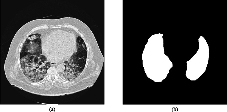
Lungs, principal components of the respiratory system in human body, are highly susceptible to diseases, where lung cancer is one of the malignant tumors with highest morbidity and mortality [1]. Lung segmentation of CT images is a precursor to most pulmonary image analysis applications and it plays an important role in computer-aided pulmonary disease diagnostics. However, accurate lung segmentation is still a challenging issue in thoracic CT image analysis due to lung shape variances, image noises, highly varied properties of pulmonary diseases, and so on (see Fig. 1). Research showed that 5–17% of lung nodules in their sampled data were missed due to the inaccurate lung segmentation [2].
Fig. 1.
A thoracic CT image (a) with its segmented lung mask (b). The uneven grayscale distribution of the image caused by pathological abnormities makes lung segmentation a difficult task
Conventional methods for lung segmentation, such as thresholding, region growing, watershed, and active contour, depend largely on a large difference of gray-scale values between lung regions and their surrounding tissues in thoracic CT images. The methods are easily influenced by image noises and usually fail to segment lungs from the images corrupted by outliers and dense pathologies because of a poor target/background contrast and unwanted background clutters in the images [3]. Feature-based machine learning techniques, e.g., fuzzy c-means (FCM), k-means and random forest (RF), are widely used for medical image segmentation. However, the effects of feature-based machine learning techniques heavily rely on prior feature definition and selection [4]. Accordingly, inappropriate features may lead to inaccurate segmentation results. In recent years, deep learning techniques have been developed and applied in medical image segmentation [5]. The techniques can learn the relationship between input and output directly from a large amount of sample data without prior feature selection. Nevertheless, most schemes are constructed on image patches to perform pixel-based image classification, which often leads to expensive time consumption.
In this paper, we propose a deep learning-based segmentation architecture for lung segmentation of thoracic CT images. Instead of pixel-based image segmentation, our patch-based segmentation with deep convolutional neural network (DCNN) structure incorporates a two-pass contour refinement operation. Therefore, the time cost of lung segmentation greatly decreases and meanwhile, the accuracy of segmentation increases. Furthermore, our patch-wise identification of lungs can be achieved by the trained DCNN without any feature generating work. The basic pipeline of our algorithm is illustrated in Fig. 2.
Fig. 2.
Pipeline of our algorithm. Our algorithm covers two stages: lung segmentation based on deep convolutional neural network and contour refinement with superpixel and edge direction tracing techniques
The remainder of this paper is organized as follows: In the “Related Work” section, we introduce the related work to our algorithm. In the “Methods” section, we present a description of our DCNN model followed by a detailed introduction of our lung segmentation based on DCNN classification and two-pass contour refinement. In the “Experiments” section, we provide a set of experimental results and in the “Discussion” section, we make a further discussion on the capabilities of our segmentation framework and draw a brief conclusion in the “Conclusion” section.
Related Work
So far, researchers have presented various methods on lung CT image segmentation. Sahu et al. [6] proposed a fuzzy c-means (FCM)-based lung segmentation model. In the model, grayscale masked images of CT slices were first generated with the FCM approach and lungs were then segmented by applying a threshold method. Finally, lung contours were smoothed with morphological closing operation for including juxta-pleural nodules. Gomathi et al. [7] segmented noised lung images by modifying the distance measurement of the FCM algorithm to permit the labeling of a pixel to be influenced by other pixels while restraining the noise effect during segmentation. In [8], the thorax region was first extracted from CT images with a thresholding-based method, and structures outside the thorax region were segmented by region growing method. Initial lung region was then captured by combining the results of the two steps above and lung contours were reconstructed with a rolling ball approach. In [9], lung regions were segmented with a threshold CT level automatically determined from the histogram of the entire body region, and outlines of segmented lungs were smoothed by morphological closing operation. In order to improve the segmentation accuracy of pathological lungs, Mansoor et al. [10] took neighboring prior constraints into account in their lung segmenting. In the model, initial lung regions were first segmented by a fuzzy connectedness image segmentation algorithm and abnormal imaging patterns were then detected with a set of texture features. The segmentation was further completed by a neighboring anatomy-guided segmentation approach to cover abnormalities with weak textures and pleura regions. Alin et al. [11] aimed at accurate segmentation of pathological lungs of CT images. A fuzzy connectedness segmentation algorithm was employed for initial lung segmentation, and a random forest classifier was used to refine the segmentation with a group of textural features extracted from non-overlapping regions of interest in thoracic CT images. Esra et al. [12] developed a histogram-based k-means algorithm for lung region segmentation, where image histogram values were used to calculate distances between pixels instead of using Cartesian system of the traditional k-means method. In [13], lungs were segmented with the random forest (RF) and the segmentation results were refined by a set of postprocessing operations. In [14], initial lung mask was first segmented with thresholding, flood filling combining with 3D labeling methods, then lung boundaries characterized with a bidirectional differential chain encoding method were refined by a support vector machine (SVM) classifier. Liu et al. [15] presented a lung segmentation algorithm based on RF classifier with a set of features extracted from superpixels, and lung contours were corrected with a circle tracing technique. In [16], FCM, gray-level co-occurrence matrix, gray-level run length matrix, and histogram methods were implemented to extract features from regions of interest in thoracic CT images. The features were applied to a convolutional neural network (CNN) classifier to detect lung nodules and label pathological and normal lung tissues. Park et al. [17] applied U-Net to segment lungs from high-resolution computed tomography (HRCT) images. Islam et al. [18] proposed a lung segmentation method of chest X-ray images using a U-Net architecture with 512 × 512-dimensional inputs. In [19], a lung CT image with a fixed size of 512 × 512 was split into smaller patches with same size. Then, k-means clustering algorithm was applied to generate labeled dataset using the mean and minimum intensities of image patches. A CNN model trained with the image patches and label set was finally utilized to separate real lung parenchyma from non-lung parenchyma.
Methods
Our lung segmentation covers two main stages: lung segmentation based on DCNN model and a two-pass contour refinement of local and global.
Lung Segmentation Based on DCNN
Deep learning refers to a machine learning method that is based on a neural network model with multiple levels of data representation. CNNs are feedforward neural networks with deep structure and convolution calculation [20]. The hidden layers of a basic CNN model are usually composed of convolutional layers, pooling layers, and fully connected layers [21].
Convolutional layers serve as feature extractors, and they automatically learn the feature representations of input images. In the k th layer, the j th output feature map, , can be computed by [22].
| 1 |
where xi and yi are the i th input feature map and the j th output feature map, respectively; w is a convolutional kernal and b the bias; The multiplication sign, ∗, refers to a 2D convolutional operator, which is used to calculate the inner product of the filter model at each location of the input image; f(⋅) is a nonlinear activation function, which allows for the extraction of nonlinear features.
Pooling aggregation layers propagate the representation of input values of a small neighborhood of an image to the next layer:
| 2 |
where the output of the pooling operation, P(⋅), associated with the j th feature map, is denoted by . It lowers the computational burden by reducing the number of connections between convolutional layers.
Fully connected layers located at last hidden layer in CNN architecture interpret these feature representations.
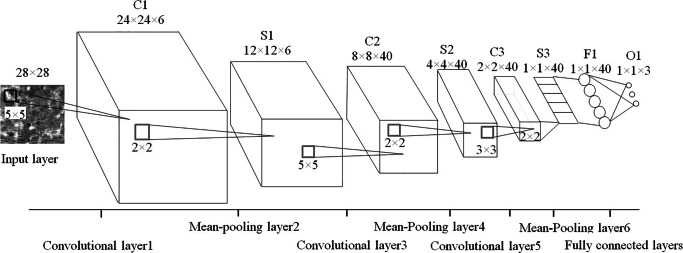
We construct an eight-layer DCNN for lung tissue classification as depicted in Fig. 3. The input image patches are resized into 28 × 28 pixels. Three convolutional layers consisted of 6, 40, and 40 kernels with sizes of 5 × 5, 5 × 5, and 3 × 3, respectively. Each kernel produces a 2D feature map and each convolutional layer is followed by a 2 × 2 mean-pooling layer with a stride of 2, which reduces the size of feature maps into 1/4 of them. Fully connected layers utilize the sigmoid function to execute nonlinear transformation from input to output with a 40-dimensional feature vector. The maximum iteration number is empirically set to 13 with a patch size of 10. The other parameters are the same as the default settings suggested in the deep learning toolbox [23].
Fig. 3.
Our DCNN structure. It covers eight layers including three convolutional layers (C1C3), three pooling layers (S1S3), a fully connected layer (F1) and an output layer (O1)
We extract lung regions, background regions, and pleural tissue regions from thoracic CT images according to ground truths. Image patches captured from these three kinds of regions are resized and taken as training and testing input datasets of our DCNN model. The output labels are valued 1, 2, and 3, which represent three kinds of regions in thoracic CT images mentioned above. After training and testing, our DCNN model is constructed for lung segmentation.
In lung segmenting with our DCNN model, an input image is equally divided into a set of non-overlapping image patches with a size of r × r. These patches are classified into three classes, lungs, backgrounds, and pleural tissues by our trained DCNN model. Lungs and backgrounds usually share similar intensity distributions especially in the images with homogenous intensities. In order to improve the segmentation accuracy, the lungs and backgrounds with lower intensities are merged into one class in the output of our algorithm, and pleural tissues are classified into another class with higher intensities. The initial binary lung mask is extracted by subtracting the background region and performing morphological operations on classification results of the DCNN model.
Two-Pass Contour Refinement
Image patch-based segmentation often produces serrated contours in the initial binary lung mask as displayed in Fig. 4. In order to smooth the jagged contours and capture accurate contours, we use a superpixel-based method to refine local contours and an edge direction tracing technique to refine global contours of lungs.
Fig. 4.
Lung segmentation with our DCNN model. Lungs of a thoracic CT image (a) and corresponding segmented binary lung mask image (b)
Local Contour Refinement with Superpixel-Based Method
A superpixel is a group of adjacent pixels with similar characteristics, such as color, brightness, or texture. It retains effective local contour information for further image segmentation. After the initial segmentation with a superpixel approach, the image is divided into a number of independent sub-regions (superpixels) (see Fig. 5 for a reference).
Fig. 5.
Segmentation results and their local close-ups created by original SLIC approach (a) and our modified SLIC approach (b)
In our algorithm, simple linear iterative clustering (SLIC) [24] is used to segment CT images into a set of superpixels. In SLIC, a k-means-based technique is used to build local clusters of pixels. Each pixel in SLIC is described with a five-dimensional vector [l, a, b, x, y]T, defined by L, a, b in CIE LAB color space and pixel coordinates, (x, y). Distances between pixels in a 2S × 2S range around each clustering center of an image patch sized S × S and their corresponding clustering center are used to determine the nearest cluster centers of pixels. The distance, D, covering space distance, ds, and color distance, dc, is defined as
| 3 |
where m is a parameter ranged from 1 to 40. ds and dc are defined as
| 4 |
| 5 |
Because the SLIC approach can generate approximately equally sized superpixels with boundaries aligning to local image edges, we refine lung local contours according to corresponding superpixel contours. However, the uneven grayscale distributions in original thoracic CT images usually lead to inaccurate superpixel contours (see Fig. 5a). In order to overcome this issue, we first smooth the image by performing an erosion and an opening morphological operation using a template of 51-dimensional vector with all 1 components on CT images, and then, we do a reconstruction operation using the gray-scale reconstruction approach of [25]. We further modify l in five-dimensional vector [l, a, b, x, y]T in SLIC approach by performing non-anisotropic diffusion filtering on it [26]:
| 6 |
where t is the number of iterations and cNx, y, cSx, y, cEx, y, and cWx, y are thermal conductivities in the four directions: top, bottom, right, and left and defined as:
| 7 |
where ∇ is a gradient operator and , , , and . k is a thermal conductivity controlling image smoothness. We empirically set t = 20, λ = 0.25, and k = 15.
Finally, we obtain more accurate superpixel contours with our modified SLIC approach (see Fig. 5b).
We map the superpixel contours into our initial lung segmentation mask and classify the superpixels into three categories. The superpixel located in the non-lung region is named black point, while that located entirely in lung region is called white point in this paper. Seeing Fig. 6a for a reference, superpixel i is a black point and j is a white point. The superpixels along the lung boundaries are partially located in lung region and they are called gray points, such as the point S0 and in Fig. 6a and c, respectively. We propose an adjacent point statistics method to smooth and refine the local lung contours by classifying gray points into white or black points shown in Algorithm 1. In the algorithm, we empirically set parameters β = 80, α1 = 0.8, α2 = 0.6, α3 = 0.5.

Fig. 6.
Local contour refinement with superpixel-based method. Point i, j in (a) are black and white points, respectively. S0 located in lung junction (a) and located on lung boundary (c) are classified into black point (b) and white point (d) by our neighborhood point statistics method, respectively
Global Contour Refinement with Edge Tracing Technique
Some lesions (e.g., juxta-pleural nodules) having similar intensities with pleural tissues, are usually excluded from segmented lung regions in lung segmenting [14]. We analyze the lung segmentation results of thoracic CT images with juxta-pleural lesions and find that the concave region of lung mask caused by a juxta-pleural lesion usually has a pair of sharp corners, and in contrast, a normal concave region often has gentle corners. Accordingly, we propose a contour correction approach based on an edge direction tracing technique to capture pairwise sharp corners and refine lung global contours. The binary lung mask is first smoothed with morphological operations in order to reduce the influence of noises. The sharpness of a point (corner) is measured by the direction difference between two adjacent points around it on lung contours. If the difference value is bigger than a threshold, the point is taken as a valid corner. Valid corner pairs are connected to repair concave regions. The main steps of the global contour refinement are shown as following:
-
Step 1.
Extract continuous single-pixel-wide lung contours from the lung mask.
-
Step 2.
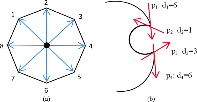
Calculate the direction, di, of each point, i, on lung contours. di is aligned to one of eight directions (see Fig. 7 for a reference).
-
Step 3.
Select an initial point, pk, from a lung contour. Calculate the direction difference △ between points pi and pj with σ pixels away from pk, respectively.
-
Step 4.Correct △ as
8 -
Step 5.
Capture valid corners. If △ satisfies the condition △≥ τ, the point pk, located in the middle of pi and pj is taken as a valid corner and put into valid corner set P0, P0 ⇐ P0 ∪{pk}.
Parameters, σ and τ, determine the sharp degree of corners. The smaller σ and bigger τ are, the shaper the corner is. We empirically set σ = 3 and τ = 3.
-
Step 6.
Count the number of points, n, in P0, P0 = {p1, p2, p3⋯pn}. If n is an odd number, there is an isolated point to be eliminated. Calculate the sum of distances between pi(i = 1⋯n) and the rest of points in P0, and find the
pm, m ∈ [1, n] with biggest distance sum and delete it from P0, P0 ⇐ P0 ∖{pm}.
-
Step 7.
Trace along lung contour in clockwise order. Record the pairwise successive two corner points (xi, yi) with △ < 0 and (xj, yj) with △ > 0, put them into set P1. P1 ⇐ P1 ∪{(xi, yi),(xj, yj)}.
-
Step 8.
Connect pairwise points in P1.
-
Step 9.
Perform morphological closing operation and a moving average filter with a span of 20 on repaired lung contours.
Fig. 7.
Point direction calculation. Direction of a point on lung contours is aligned to one of eight directions (a), points p1, p2, p3, and p4, have directions d1, d2, d3, and d4 in clockwise order, respectively (b)
Experiments
We test our algorithm on a set of experimental data from interstitial lung diseases (ILDs) database [27]. It contains high-resolution computed tomography (HRCT) image series with pathologically proven diagnoses of ILDs. The images in the ILDs database and the corresponding lung contours corrected by radiologists are taken as the testing dataset of our algorithm.
Evaluation Method
A group of metrics are used to evaluate our lung segmentation performance including Sensitivity (SEN), Precision (PRE), Accuracy (ACC), Recall (REC), and Error, which are defined by True Positive (TP), False Positive (FP), True Negative (TN), and False Negative (FN):
TP: Lung instances correctly classified into the ground truth
FP: Lung instances incorrectly classified into the ground truth.
TN: Lung instances correctly recognized not to belong to the ground truth.
FN: Lung instances incorrectly classified, to not belong to the ground truth.
| 9 |
| 10 |
| 11 |
| 12 |
| 13 |
Other five classical metrics [6], over-segmentation rate (OR), under-segmentation rate (UR), Dice similarity coefficient (DSC), Jaccard’s similarity index (JSI), average symmetric surface distance (ASD), and modified Hausdorff distance (MHD), where MHD is defined as Eq. 14, are also utilized for evaluating the performance of our lung segmentation algorithm.
| 14 |
where B and A are the segmented lung region and the corresponding ground truth, respectively, and Na is the number of pixels in A.
Larger values of SEN, PRE, ACC, REC, DSC, and JSI, and smaller values of Error, UR, OR, and MHD often indicate better performance of a segmentation algorithm.
The Effects of Image Patch Size and Preset Superpixel Number on Algorithm Efficiency
Our algorithm degenerates into pixel-based classification when the image patch size, B, is set to 1. The segmentation result of pixel-based classification is similar to that of image patch-based classification as shown in Fig. 8a and b. However, their processing times are very different. For example, the average processing time of a pixel-based operation is 13 times more than that of patch-based operation for images of size 512 × 512 (see Fig. 8c for a reference).
Fig. 8.
Initial lung segmentation result. A pixel-based (a) and a patch-based (b) lung segmentation results with our DCNN model and their corresponding average processing time
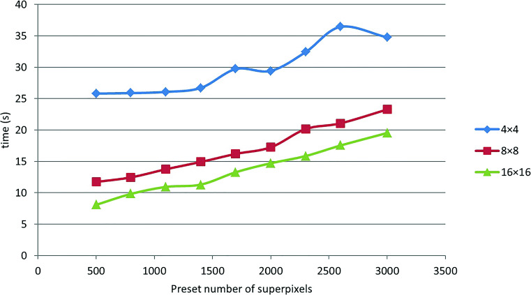
We test our algorithm with different image patch sizes, B s, and preset superpixel numbers, N s, on a set of thoracic CT images. The average processing time of an image is depicted in Fig. 9. It can be observed that the smaller the B and the bigger the N, the higher the time cost. Nevertheless, although a bigger B and a smaller N can decrease the time cost of lung segmenting, they may synchronously decrease segmentation accuracy. In the following, we analyze the relationship between B, N, and the segmentation accuracy.
Fig. 9.
Time cost of segmentation with different B s and different N s
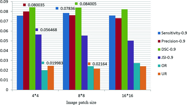
We test our algorithm with different B s and N s on 60 CT images of sarcoidosis. The results are listed in Table 1, where the best results are shown in italics. It can be observed that the lung segmentation achieves higher accuracy when N = 800. Thus, we compare the segmentation accuracies with different B s when N is 800 and the results are exhibited in Fig. 10. The best results are labeled on the bars. We can find that the values of metrics are slightly different due to the effective local contour refinement with superpixels. On the whole, the segmentation accuracies with B = 8 × 8 and B = 4 × 4 are higher than that with B = 16 × 16. We take the time cost into account and seek a balance among B, N, and segmentation accuracy, and we finally set B = 8 × 8 and N = 800 here.
Table 1.
Performance of our algorithm with different B s and different N s
| B | N | SEN | PRE | DSC | JSI | OR | UR |
|---|---|---|---|---|---|---|---|
| 4 × 4 | 500 | 0.9746 | 0.9783 | 0.9835 | 0.9538 | 0.0218 | 0.0254 |
| 800 | 0.9756 | 0.9800 | 0.9843 | 0.9565 | 0.0200 | 0.0244 | |
| 1100 | 0.9760 | 0.9789 | 0.9839 | 0.9557 | 0.0212 | 0.0240 | |
| 1400 | 0.9772 | 0.9784 | 0.9846 | 0.9564 | 0.0218 | 0.0228 | |
| 1700 | 0.9772 | 0.9784 | 0.9844 | 0.9565 | 0.0217 | 0.0228 | |
| 2000 | 0.9778 | 0.9780 | 0.9844 | 0.9566 | 0.0222 | 0.0222 | |
| 2300 | 0.9783 | 0.9783 | 0.9849 | 0.9574 | 0.0218 | 0.0217 | |
| 2600 | 0.9766 | 0.9778 | 0.9840 | 0.9553 | 0.0223 | 0.0234 | |
| 3000 | 0.9777 | 0.9775 | 0.9843 | 0.9560 | 0.0227 | 0.0223 | |
| 8 × 8 | 500 | 0.9766 | 0.9755 | 0.9828 | 0.9531 | 0.0249 | 0.0234 |
| 800 | 0.9784 | 0.9761 | 0.9840 | 0.9553 | 0.0241 | 0.0216 | |
| 1100 | 0.9791 | 0.9751 | 0.9839 | 0.9550 | 0.0253 | 0.0209 | |
| 1400 | 0.9789 | 0.9749 | 0.9837 | 0.9547 | 0.0254 | 0.0211 | |
| 1700 | 0.9797 | 0.9728 | 0.9832 | 0.9534 | 0.0277 | 0.0203 | |
| 2000 | 0.9797 | 0.9741 | 0.9837 | 0.9546 | 0.0263 | 0.0203 | |
| 2300 | 0.9804 | 0.9633 | 0.9790 | 0.9445 | 0.0403 | 0.0196 | |
| 2600 | 0.9796 | 0.9713 | 0.9827 | 0.9518 | 0.0293 | 0.0204 | |
| 3000 | 0.9796 | 0.9615 | 0.9780 | 0.9421 | 0.0421 | 0.0204 | |
| 16 × 16 | 500 | 0.9776 | 0.9637 | 0.9788 | 0.9426 | 0.0384 | 0.0224 |
| 800 | 0.9759 | 0.9732 | 0.9823 | 0.9502 | 0.0273 | 0.0241 | |
| 1100 | 0.9784 | 0.9537 | 0.9760 | 0.9335 | 0.0500 | 0.0216 | |
| 1400 | 0.9807 | 0.9410 | 0.9706 | 0.9232 | 0.0660 | 0.0193 | |
| 1700 | 0.9794 | 0.9426 | 0.9718 | 0.9238 | 0.0623 | 0.0206 | |
| 2000 | 0.9803 | 0.9310 | 0.9667 | 0.9131 | 0.0774 | 0.0197 | |
| 2300 | 0.9788 | 0.9375 | 0.9694 | 0.9182 | 0.0683 | 0.0212 | |
| 2600 | 0.9801 | 0.9184 | 0.9606 | 0.9007 | 0.0940 | 0.0199 | |
| 3000 | 0.9789 | 0.9236 | 0.9627 | 0.9046 | 0.0867 | 0.0211 |
Fig. 10.
Performance of our algorithm with different B s and N = 800 with the best results labeled on the bars
Result Analysis
We test our algorithm on five sets of thoracic CT images in the interstitial lung diseases (ILDs) dataset: ground glass (G), fibrosis (F), healthy (H), sarcoidosis (S), and reticulation (R). It is noticed that because the number of CT cases with different diseases varies a lot and our algorithm is suitable for slice-based lung segmentation, accordingly, the evaluation is performed on a set of CT slices. As an example, a set of results are shown in Fig. 11.
Fig. 11.
Lung segmentation. For thoracic CT images (a), lungs are initially segmented with our DCNN model (b). With our adjacent point statistics method based on superpixels, we locally refine the segmented lung contours in (c). The final lung segmentation results (d) are obtained by the second pass refinement of contours based on edge direction tracing
We evaluate the segmentation performances of three main steps of our algorithm in terms of DSC, JSI, Error, and MHD, and the results are shown in Figs. 12 and 13. The main three steps include lung segmentation, local contour refinement, and global contour refinement; the corresponding metrics are DSC1, JSI1, DSC2, JSI2, DSC3, and JSI3 in Fig. 12. From Fig. 12 we can see that the local refinement can greatly improve the lung segmentation accuracy. Global refinement approach can improve the segmentation accuracies of G, F, and S images with inhomogeneous intensities. Nevertheless, the accuracy becomes a little bit lower for H and R images with homogenous intensities because our local contour refinement operation has already produced smooth contours, and the global contour refinement brings a little over-segmentation. Figure 13a shows the segmentation accuracy of F images with inhomogeneous intensities and H images with homogeneous intensities in terms of MHD. Our algorithm can segment lung images well, especially for the ones having uneven gray-scale distributions. The average Error and MHD of the dataset are depicted in Fig. 13b. The Error is greatly reduced after the local and global contour refinements. Although MHD of the third step (global contour refinement) is a little bit higher than that of the second step, global contour refinement plays an import part in the lung segmentation of intensity inhomogeneous images for the segmentation of juxta-pleural nodules and other pathological focus which share similar intensity distributions with pleural tissues.
Fig. 12.
Performance evaluation of three main steps of our algorithm on five types of images, G, F, H, S, and R. DSC1DSC3 (a) and JSI1JSI3 (b) are respectively the segmentation accuracies of lung segmentation, local contour refinement and global contour refinement in terms of DSC and JSI
Fig. 13.
Performance evaluation of three main steps of our algorithm in terms of Error and MHD. a MHDs of F and H images and b average Error and MHD of G, F, H, S, and R images
In Table 2, we exhibit the segmentation accuracies on G, F, H, S, and R images. It can be seen that the average Precision, Accuracy, DSC, and JSI are 0.9725, 0.9924, 0.9795, and 0.9448, respectively. Figure 14 gives the MHD and Error values of our algorithm on five types of images. H images have lower MHD and Error than other types of images due to the homogeneous intensities. On the contrary, F and S images have higher MHD and Error because of inhomogeneous intensities of the images.
Table 2.
Performance of our algorithm on five types of thoracic CT images
| Types | PRE | ACC | SEN | REC | DSC | JSI | ASD | OR | UR |
|---|---|---|---|---|---|---|---|---|---|
| G | 0.9772 | 0.9911 | 0.9561 | 0.9561 | 0.9764 | 0.9349 | 0.4107 | 0.0226 | 0.0439 |
| F | 0.9598 | 0.9894 | 0.9401 | 0.9401 | 0.9640 | 0.9060 | 0.6450 | 0.0395 | 0.0599 |
| H | 0.9794 | 0.9958 | 0.9946 | 0.9946 | 0.9945 | 0.9874 | 0.0815 | 0.0210 | 0.0054 |
| S | 0.9731 | 0.9910 | 0.9643 | 0.9643 | 0.9778 | 0.9398 | 0.4042 | 0.0277 | 0.0357 |
| R | 0.9732 | 0.9947 | 0.9818 | 0.9818 | 0.9849 | 0.9557 | 0.3036 | 0.0276 | 0.0182 |
| A | 0.9725 | 0.9924 | 0.9674 | 0.9674 | 0.9795 | 0.9448 | 0.3690 | 0.0277 | 0.0326 |
Fig. 14.
Performance of our algorithm in terms of MHD (a) and Error (b)
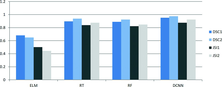
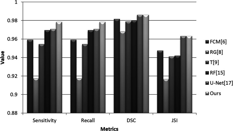
Features extracted from the gray-level co-occurrence matrix (GLCM) are widely used for object identification and classification [28]. Combining with GLCM features and intensity features of mean, variance, and skewness, after we divide the input image into a set of non-overlapping image patches with a size of r × r, we classify the image patches with extreme learning machine (ELM), regression tree (RT), random forest (RF), and our algorithm on 60 F images randomly selected from thoracic CT images, respectively. The initial results are further improved with our two-pass contour refinement method. The corresponding results are listed in Fig. 15. DSC1 and JSI1 and DSC2 and JSI2 indicate the segment accuracies before and after refinement operation, respectively. It can be seen that the performance of our DCNN model-based segmentation algorithm is better than those of other methods in terms of DSC and JSI. RT and RF methods achieved higher accuracy than ELM, and our two-pass contour refinement method can improve their segmentation results. Because ELM produced bad classification results, where the segmented lung regions are incomplete and discrete. Accordingly, some discrete regions are mistaken as invalid ones and eliminated by our refinement method, which caused that DSC2 and JSI2 are lower than DSC1 and JSI1, respectively. All in all, the deep learning neural network outperforms the traditional classifiers in this case. Additionally, we make a comparison of segmentation accuracy between our algorithm and a set of current methods shown in Fig. 16. The images are randomly selected from F and S images. It can be seen that the accuracy of our algorithm is higher than FCM [6], RG (region growing) [8], T (thresholding) methods [9], RF [15], and U-Net [17] in terms of Sensitivity and Recall. FCM, RG, and T are good for segment intensity homogeneous images but failed to segment those with uneven distribution of intensities. U-Net’s DSC and JSI are similar to ours with the same training (1000) and testing samples (100). Nevertheless, the Sensitivity and Recall of ours are higher than U-Net’s.
Fig. 15.
Performance comparison on lung segmentation of four methods, ELM, RT, RF, and our methods (DCNN). DSC1 and JSI1 and DSC2 and JSI2 indicate the segment accuracies before and after refinement operation, respectively
Fig. 16.
Performance comparison of several current lung segmentation methods
Discussion
Pathologic lungs suffered from some diseases, such as pneumocystis pneumonia and pulmonary fibrosis, usually have similar intensities with pleural tissues. The pathological lung regions along with normal lung regions are extracted and taken as the training data of our DCNN model. Because of the smaller lung CT image data set, DCNN model sometimes cannot distinguish lung regions from pleural tissues. Therefore, in some segmentation results, partial pleural tissues having similar intensities with pathological lungs are classified into lung regions (see Fig. 17 for a reference). One solution to this problem is to augment training samples of DCNN model, the other solution is to employ some techniques to remove the pleural tissues from initial segmentation results. In this paper, we adopt the second solution with a region matching approach. For example, for a thoracic CT image (Fig. 17a), the initial segmentation result (Fig. 17b) involves some pleural tissues locating around the thorax. We extract the chest boundary (Fig. 17c) from the segmented chest region and eliminate the regions connected with chest boundary. After two-pass contour refinements, we obtain the final segmented lung mask (Fig. 17d). In some initial segmentation cases, lungs are connected with pleural tissues and we can employ an erode operation to separate them in advance, and then eliminate lung tissues with above processing operations.
Fig. 17.
Pleural tissue elimination. For a thoracic CT image (a), we extract initial lung region (b) with our DCNN model. Regions connected to chest boundary (c) are removed from (b), and final lung region mask (d) is extracted by two-pass contour refinement operation
Conclusion
Deep learning techniques are widely used in object detection and classification without feature selecting. In this paper, we introduce a deep convolutional neural network to segment the lungs from thoracic CT images. In order to accelerate the segmentation, we use a non-overlapping image patch-based strategy instead of pixel-based approaches to classify lungs with our DCNN model. Superpixels are used to smooth serrated local contours. With an edge direction tracing technique, the global lung contours are corrected and our algorithm achieves high accuracy. In future work, we will augment training samples and improve DCNN architecture to further enhance lung segmentation accuracy.
Funding
The work in this paper was supported by grants from the National Natural Science Foundation of China (Grant Nos. 41631175, 61702068), the Key Project of Ministry of Education for the 13th 5-years Plan of National Education Science of China (Grant No. DCA170302), the Social Science Foundation of Jiangsu Province of China (Grant No. 15TQB005), the Priority Academic Program Development of Jiangsu Higher Education Institutions (Grant No. 1643320H111) and the Postgraduate Research & Practice Innovation Program of Jiangsu Province (Grand No. KYCX19_0733).
Compliance with Ethical Standards
Conflict of Interest
The authors declare that they have no conflict of interest.
Footnotes
Publisher’s Note
Springer Nature remains neutral with regard to jurisdictional claims in published maps and institutional affiliations.
Contributor Information
Caixia Liu, Email: cxsqz@126.com.
Mingyong Pang, Email: panion@netease.com.
References
- 1.Zhou S, Cheng Y, Tamura S. Automated lung segmentation and smoothing techniques for inclusion of juxtapleural nodules and pulmonary vessels on chest CT images. Biomed Signal Process Control. 2014;13:62–70. doi: 10.1016/j.bspc.2014.03.010. [DOI] [Google Scholar]
- 2.Armato S, III, Sensakovic W. Automated lung segmentation for thoracic CT: impact on computer-aided diagnosis1. Acad Radiol. 2004;11(9):1011–1021. doi: 10.1016/j.acra.2004.06.005. [DOI] [PubMed] [Google Scholar]
- 3.Sluimer I, Prokop M, Van Ginneken B. Toward automated segmentation of the pathological lung in CT. IEEE Trans Medical Imag. 2005;24(8):1025–1038. doi: 10.1109/TMI.2005.851757. [DOI] [PubMed] [Google Scholar]
- 4.Hu Z, Tang J, Wang Z, et al. Deep learning for image-based cancer detection and diagnosis- a survey. Pattern Recognit. 2018;83:134–149. doi: 10.1016/j.patcog.2018.05.014. [DOI] [Google Scholar]
- 5.Litjens G, Kooi T, Bejnordi B, et al. A survey on deep learning in medical image analysis. Med Image Anal. 2017;42:60–88. doi: 10.1016/j.media.2017.07.005. [DOI] [PubMed] [Google Scholar]
- 6.Sahu S, Agrawal P, Londhe N, et al. A new hybrid approach using fuzzy clustering and morphological operations for lung segmentation in thoracic ct images. Biomed Pharmacol J. 2017;10(4):1949–1961. doi: 10.13005/bpj/1315. [DOI] [Google Scholar]
- 7.Gomathi M, Thangaraj P. A new approach to lung image segmentation using fuzzy possibilistic c-means algorithm. Int J Comput Sci Inf Secur. 2010;7(3):14–24. [Google Scholar]
- 8.Santos A, de Carvalho Filho A, Silva A, et al. Automatic detection of small lung nodules in 3D CT data using Gaussian mixture models, Tsallis entropy and SVM. Eng Appl Artif Intell. 2014;36:27–39. doi: 10.1016/j.engappai.2014.07.007. [DOI] [Google Scholar]
- 9.Arimura H, Katsuragawa S, Suzuki K, et al. Computerized scheme for automated detection of lung nodules in low-dose computed tomography images for lung cancer screening. Acad Radiol. 2004;11(6):617–629. doi: 10.1016/j.acra.2004.02.009. [DOI] [PubMed] [Google Scholar]
- 10.Mansoor A, Bagci U, Xu Z, et al. A generic approach to pathological lung segmentation. IEEE Trans Med Imaging. 2014;33(12):2293–2310. doi: 10.1109/TMI.2014.2337057. [DOI] [PMC free article] [PubMed] [Google Scholar]
- 11.Alin Mercybha P, Brinda T. Intelligent pathological lung segmentation using random forest machine learning. Int J Innov Res Comput Commun Eng. 2015;3(3):21–26. [Google Scholar]
- 12.Dincer E, Duru N: Automatic lung segmentation by using histogram based k-means algorithm.. In: Proceedings of International Conference on Electric Electronics, Computer Science, Biomedical Engineerings Meeting, 2016, pp 1–4
- 13.Liu C, Zhao R, Pang M. A fully automatic segmentation algorithm for CT lung images based on random forest. Med Phys. 2020;47(2):518–529. doi: 10.1002/mp.13939. [DOI] [PubMed] [Google Scholar]
- 14.Shen S, Bui A, Cong J, et al. An automated lung segmentation approach using bidirectional chain codes to improve nodule detection accuracy. Comput Biol Med. 2015;57:139–149. doi: 10.1016/j.compbiomed.2014.12.008. [DOI] [PMC free article] [PubMed] [Google Scholar]
- 15.Liu C, Zhao R, Pang M. Lung segmentation based on random forest and multi-scale edge detection. IET Image Process. 2019;13(10):1745–1754. doi: 10.1049/iet-ipr.2019.0130. [DOI] [Google Scholar]
- 16.Jalal D, Ganesan R, Merline A. Fuzzy-c-means clustering based segmentation and CNN-classification for accurate segmentation of lung nodules. Asian Pac J Cancer Prev Apjcp. 2017;18(7):1869–1874. doi: 10.22034/APJCP.2017.18.7.1869. [DOI] [PMC free article] [PubMed] [Google Scholar]
- 17.Park B, Park H, Lee S, et al. Lung segmentation on HRCT and volumetric CT for diffuse interstitial lung disease using deep convolutional neural networks. J Digital Imaging. 2019;32(6):1019–1026. doi: 10.1007/s10278-019-00254-8. [DOI] [PMC free article] [PubMed] [Google Scholar]
- 18.Islam J, Zhang Y (2018) Towards robust lung segmentation in chest radiographs with deep learning. arXiv:1811.12638, 1–5
- 19.Xu M, Qi S, Yue Y, et al. Segmentation of lung parenchyma in CT images using CNN trained with the clustering algorithm generated dataset. Biomed Eng Online. 2019;18(1):1–21. doi: 10.1186/s12938-018-0619-9. [DOI] [PMC free article] [PubMed] [Google Scholar]
- 20.Tajbakhsh N, Suzuki K. Comparing two classes of end-to-end machine-learning models in lung nodule detection and classification: MTANNS vs. CNNS. Pattern Recognit. 2017;63:476–486. doi: 10.1016/j.patcog.2016.09.029. [DOI] [Google Scholar]
- 21.LeCun Y, Bottou L, Bengio Y, et al. Gradient-based learning applied to document recognition. Proc IEEE. 1998;86(11):2278–2324. doi: 10.1109/5.726791. [DOI] [Google Scholar]
- 22.Lai Z, Deng H. Medical image classification based on deep features extracted by deep model and statistic feature fusion with multilayer perceptron. Comput Intel Neurosc. 2018;28:1–13. doi: 10.1155/2018/2061516. [DOI] [PMC free article] [PubMed] [Google Scholar]
- 23.Palm R (2014) Deeplearntoolbox, a matlab toolbox for deep learning. [Online]. Dispon⋅⋅avel em: https://github.com/rasmusbergpalm/DeepLearnToolbox
- 24.Achanta R, Shaji A, Smith K, et al. SLIC superpixels compared to state-of-the-art superpixel methods. IEEE Trans Pattern Anal Mach Intell. 2012;34(11):2274–2282. doi: 10.1109/TPAMI.2012.120. [DOI] [PubMed] [Google Scholar]
- 25.Vincent L. Morphological grayscale reconstruction in image analysis: Applications and e cient algorithms. IEEE Trans Image Process. 1993;2(2):176–201. doi: 10.1109/83.217222. [DOI] [PubMed] [Google Scholar]
- 26.Bai J, Feng X. Fractional-order anisotropic diffusion for image denoising. IEEE Trans Image Process. 2007;16(10):2492–2502. doi: 10.1109/TIP.2007.904971. [DOI] [PubMed] [Google Scholar]
- 27.Depeursinge A, Vargas A, Platon A, et al. Building a reference multimedia database for interstitial lung diseases. Comput Med Imag Grap. 2012;36(3):227–238. doi: 10.1016/j.compmedimag.2011.07.003. [DOI] [PubMed] [Google Scholar]
- 28.de Siqueira F, Schwartz W, Pedrini H. Multi-scale gray level co-occurrence matrices for texture description. Neurocomputing. 2013;120:336–345. doi: 10.1016/j.neucom.2012.09.042. [DOI] [Google Scholar]


