Future climates: Markov blankets and active inference in the biosphere

Abstract

We formalize the Gaia hypothesis about the Earth climate system using advances in theoretical biology based on the minimization of variational free energy. This amounts to the claim that non-equilibrium steady-state dynamics—that underwrite our climate—depend on the Earth system possessing a Markov blanket. Our formalization rests on how the metabolic rates of the biosphere (understood as Markov blanket's internal states) change with respect to solar radiation at the Earth's surface (i.e. external states), through the changes in greenhouse and albedo effects (i.e. active states) and ocean-driven global temperature changes (i.e. sensory states). Describing the interaction between the metabolic rates and solar radiation as climatic states—in a Markov blanket—amounts to describing the dynamics of the internal states as actively inferring external states. This underwrites climatic non-equilibrium steady-state through free energy minimization and thus a form of planetary autopoiesis.

1. Introduction

The standard models of the Sun's evolution show an increase in its radiation and brightness over time [1,2]. Yet, there is empirical and model evidence that, despite exposure to increasing radiation, the temperature of Earth's climate has remained bounded at habitable levels ≈0–40°C since the Archean (4 billion years before present) [3,4]. By contrast, Earth's climate dynamics would not be possible for its planetary lifeless neighbours—such as Mars and Venus—whose dynamics are non-habitable [5].

It has been noted since the inception of physiology that biological systems maintain their organization and bounded internal conditions in the face of external fluctuations [6]. By contrast, the entropy of inert (and closed) systems is unbounded and increases indefinitely. This asymmetry between external and internal conditions is thus broadly recognized as an important characteristic of biological systems [7,8]. Schrödinger asked about such internal conditions, how can the events in space and time which take place within the spatial boundary of a living organism be accounted for by physics and chemistry? [9, p. 2].

Recent advances in theoretical biology suggest that biological systems can resist dissipation and external fluctuations through predictive behaviour [10–12]. That is, biological systems preserve their organization and bounded internal conditions by anticipation and active inference, or at least behave as if they had these predictive faculties. The underlying observation is that the time evolution of all systems, whether they are biological or not, depends on the past. However, the time evolution of living systems looks as if it depends not only on the past and present but also on the future [10–12]. The reason for this is that living systems act on the basis of a predictive model of their ambiance: they appear to model their ambiance to preserve their organization and bounded internal conditions [10–12]. Such predictive behaviour is named anticipation [10,13–16], allostasis [11,17,18] and recently, active inference [12,19–21]. Active inference is a corollary of the free energy principle that describes the organization of systems that can be distinguished from their external milieu, in virtue of possessing a Markov blanket [12,21].

Since the asymmetry between the Earth's internal and external conditions implies some sort of action to maintain the bounded temperatures at habitable levels, we, therefore, offer the following hypothesis: can the Earth's climate system be interpreted as an anticipatory system that minimizes variational free energy? [22]. This hypothesis provides an interesting connection with the Gaia hypothesis which argues for Earth's planetary bounded internal conditions by and for the biosphere [23–25]. Here, we formalize the Gaia hypothesis by providing key organizational relationships among the atmosphere, hydrosphere, lithosphere and biosphere that allow a mathematical formulation of a Markov blanket for the Earth's climate system. This should be considered as a precondition for interpreting and proving (elsewhere) that the temperature of the Earth's climate—bounded within habitable ranges—has arisen due to an anticipatory or active (Bayesian) inference. In the following section, we briefly review the relationship between Markov blankets, free-energy minimization and active inference. We then propose, based on empirical evidence and prior model-based theoretical work, the existence of a Markov blanket for the Earth's climate system. Finally, we point out some implications of this formal treatment for studying the Earth's climate dynamics.

2. Free energy, Markov blankets and active inference

Although the principle of free energy minimization arose in neuroscience, it turned out to be sufficiently generic to ascribe cognitive processes to all living systems [12]. Thus, the minimization of free energy (a.k.a., a generalized prediction error) can be regarded as a dynamical formalization of the embodied cognition implicit in autopoiesis or biological self-production [12,26–30]. One of the conditions for the existence of an autopoietic system is a boundary [31], which resonates with Schrödinger's question above. A Markov blanket defines the boundary between a system of interest and its environment in a statistical sense. More specifically, it provides a statistical partitioning of a system into states internal and states external to the system. In this context, a Markov blanket is a set of variables through which things internal and external to a system interact.

Important examples of Markov blankets arise in multiple fields. One of the most commonly encountered is the present—which is the Markov blanket separating the past from the future and underwrites the notion of a Markov process. Markov processes [32] are stochastic (random) processes whose dynamics may be characterized without reference to their distant past. In other words, if we know the present state of a system, knowing about the past tells us nothing new about the likely future. On one reading of Newtonian physics, the positions and momenta of particles can be seen as the Markov blankets through which particles interact with one another [33]. In biology, Markov blankets have been associated with the physical boundaries surrounding cells [12,20,34] (i.e. their membrane) through which all influence between the intracellular and extracellular spaces are mediated. At larger spatial scales, they have been drawn around plant neurobiology [35] and neural networks [36] such that the superficial and deep pyramidal cells of the cerebral cortex play the role of a Markov blanket, through mediating interactions between different cortical columns. This concept has been extended to a number of spatial scales [19], with muscles and sensory receptors acting as an organism's Markov blanket, and specific organisms acting as blankets to separate groups of organisms. The thing all of these examples have in common is that they separate the world into two sets of states, which interact only via their Markov blanket [37].

Pearl [38] introduced the term ‘Markov blanket’ to describe the set of variables that mediate relationships to and from a variable of interest. More precisely, for a given variable X and its known blanket states b, no more information about X is gained when knowing the state of variables outside b. This does not imply that knowing the blanket states allows one to fully predict the evolution of the target variable. This is because there may be some intrinsic properties in the system that renders X stochastic. Markov blankets segregate ‘directed graphs’ known as Bayesian networks such that one side of the blanket is conditionally independent of the other, given the blanket. This conditional independence clearly has important existential implications.

The Markov blankets that one considers in active inference, comprise sensory and active states, that feature specific coupling or causality relationships with internal and external states [12,21] (figure 1). Here, the term ‘states’ stands for any variable of the system. A stipulative condition for the existence of a Markov blanket is that internal states must be conditionally independent of external states, given blanket states and vice versa. This formalizes the idea that there are no direct interactions between internal and external states, only via the blanket states. In other words, internal and external states can only influence one another via sensory and active states and the internal states only ‘see’ the external states through the ‘veil’ of the Markov blanket [12,21]. Specifically, active states mediate the influence of internal states on external states, and sensory states mediate the reciprocal influences. In other words, internal states cannot influence sensory states, while external states cannot influence active states [12,21] (figure 1). The conditional independence between internal and external states—provided by blanket states—enables interactions between the inside and outside of the system, but only via the blanket. It is worth noting that the terms ‘active’ and ‘sensory’ derive from applications of this formalism to biology. However, the same mathematical relations exist in Hamiltonian dynamics, where these may be replaced with the labels ‘position’ and ‘momentum’.

Figure 1.

Markov blankets and active inference. (a,b) The partition of states into internal states and hidden or external states that are separated by a Markov blanket—comprising sensory and active states in the brain and in a cell, respectively. (a) For the assignation of states in the brain, see [33,34]. (b) The internal states can be associated with the intracellular states of a cell, while sensory states become the surface states of the cell membrane overlying active states (e.g. the actin-like MreB filaments [39] that mediate cell mobility). The intracellular state dynamics of a cell correspond to perception, while action mediates coupling from internal states to external states. Importantly, once such a Markov blanket is established for a system of interest, along with the necessary condition of non-equilibrium steady state (NESS), one can formally show that the internal states predict external states and thereby self-maintain the system, via a minimization of variational free energy [33,40]. This, in turn, implies that the expected entropy of sensory states remains bounded, thereby ensuring resistance to dissipation by external fluctuations. Note that s here is assumed to be given by a static function of x. The underlying reason for this is that most software implementations use g to specify a likelihood of sensations given external states, under an adiabatic approximation to the underlying dynamics.

Active inference is, thus, an account of autopoiesis in dynamic terms, provided that such systems are (i) at non-equilibrium steady state (NESS) and (ii) that can be statistically segregated from their environment as in figure 1. The first NESS condition simply means that a system persists over a non-trivial timescale and does not dissipate. This implies the existence of a NESS density to which the system self-organizes that can be thought of as a probabilistic description of the system's pullback attractor [39,40]. The second (statistical segregation) condition implies the presence of a Markov blanket [20,38]. The NESS dynamics of the system—and the presence of the conditional independencies implied by a Markov blanket—means that the average internal state effectively parameterize a probability distribution over the external states [12,20,33,41]. In other words, for any given blanket state, the average internal state represents the causes (i.e. hidden, or external) of sensory impressions. It is fairly straightforward to show that the dynamics of the (average) internal state constitute a gradient flow on a variational free energy functional of this parameterized density. The minimization of free energy (and implicit minimization of sensory entropy) enables biological systems to maintain their sensory states within physiological bounds, and undertake predictive behaviour about the causes of their sensation necessary to sustain their existence [12,21,42].

In this context, minimization of free energy means resisting entropic fluctuation and maintenance of a bounded set of physiological states. As free energy is a functional of a probabilistic model (the parameterized density over external states above), this means a system must instantiate an implicit model of its ambient space. Minimizing free energy fits such a model to sensory states, thereby ensuring good predictive behaviour. In Bayesian statistics, the evidence for such a model is known as the ‘model’ evidence or marginal likelihood: namely, the probability of observing some data, given a model of how those data were generated. Variational free energy upper bounds the negative log model evidence, which is a ubiquitous quantity in statistical physics, Bayesian statistics and machine learning [43]. In machine learning, the variational free energy is commonly called the evidence lower bound, or ELBO [44]. In engineering, it is the cost function associated with Kalman filters. In information theory, minimizing free energy corresponds to maximizing efficiency or minimum description length approaches. In predictive coding, the evidence is taken as the (precision weighted) prediction error. Crucially, in the free energy framework these are all the same thing: the probability distribution encoded by the internal states that quantifies the dynamics of the external states and evolves towards the variational free energy minimum [45]—an upper bound on surprise or negative log evidence (i.e. the negative log probability of finding the system in a particular state) [12].

The surprise is a function of the states of the Markov blanket itself [45]. Free energy is a function of probabilistic beliefs, encoded by internal states about external states (i.e. expectations about the probable causes of sensory interaction), given any blanket state.¹ When these beliefs are equal to the posterior probability over external states, free energy becomes equivalent to surprise. Otherwise, it is always greater than (i.e. constitutes an upper bound on) surprise [45]. Vicarious interaction through a Markov blanket lends an interpretation to the dynamics of such systems, as if internal states were inferring external states based upon the blanket states. This implies that the kind of organization of Markov blankets we consider results in processes that work to seek out evidence (active inference), namely self-evidencing dynamics underlying the autopoietic—thus autonomous—organization of life [8,46].

In brief, this means we can characterize living systems as minimizing variational free energy, and therefore surprise, where the minimization of variational free energy entails the optimization of beliefs about things beyond the Markov blanket (i.e. external states). Thus, external fluctuations can therefore (or must therefore) be modelled to maintain a bounded set of physiological states. This formalism has been applied to a range of problems in biology [12,19,28,35] including thermodynamic physical systems [33,41]. On the basis of the ensuing Bayesian process of active inference, we turn next to defining and evidence-based Markov blanket for the Earth's climate system.

3. Markov blankets and the Earth's climate system

Several authors suggest that autopoiesis happens at the planetary scale [47–56]. The implication of this view is that minimization of variational free energy must also occur at the planetary level. The challenge for this perspective is to identify the Markov blanket of a climate system (here, the Earth) such that we can think about how internal states of the system may appear to infer and act upon external states. Delineating this blanket is essential in finding the generative model that determines climate dynamics. To do so, we need to define variables (i.e. states) internal and external to the Earth's climate system—those states that constitute or are intrinsic to the system and those that are not. In so doing, we regard empirical and model-evidence based interactions between the Earth's climate components and identifies a set of variables that satisfy the conditional independencies allowed by the Markov blankets that underwrite active inference (figure 2).

Figure 2.

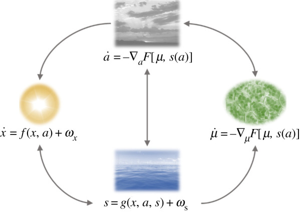
Earth's climate and Markov blankets. This figure illustrates the conditional dependencies between four key variables in the Earth's climate system. These conditional dependencies imply a Markov blanket comprising active (a) and sensory (s) states (in analogy with perception–action loops in cognitive science) that mediate the interactions between internal (μ) and external (x) states. The internal states are the metabolic rate changes of atmospheric greenhouses and aerosols turnover (see §3.2 for the full explanation). These influence active states (changes in greenhouse and albedo effects) (see §3.3) and vicariously the external states (solar radiation changes at the Earth's surface) (see §3.1). The external states cause changes in the sensory states (ocean-driven global temperature changes) (see §3.4), which leads to changes in the internal states. External (and sensory) states exhibit dynamics prescribed by stochastic differential equations (or a static stochastic mapping) with Gaussian white noise uncorrelated in time (ω). Internal and active states perform a gradient descent on variational free energy (F), defined in relation to a (characteristic) NESS density for the external and sensory states. As a consequence, the internal states appear to model and act upon the external and sensory states.

Figure 2 illustrates the conditional dependencies between variables forming the Earth's climate system and Markov blanket, highlighting that the metabolic rates of the biosphere (internal states) only influences solar radiation at the Earth's surface (external states) via changes in greenhouses and albedo effects (active states), while reciprocal interactions are mediated by the ocean-driven global temperature changes (sensory states). We turn next to defining each of these variables that constitute this climatic partition of states.

3.1. External states (x): solar radiation changes at the Earth's surface

The space weather² and external environment of the Earth system, such as the electromagnetic solar radiation and galactic cosmic shortwave radiation and energetic electron precipitation, are the source of energy, but also of external forcing and perturbation, respectively [58]. In many mainstream climate models (radiative energy balance models, earth system models of intermediate ‘complexity’ and general circulation models) cosmic rays are not a source of forcing fluctuation in the climate system. Indeed, the study of the impact of cosmic rays on Earth, in general, does not fall within climate science, but rather with astrophysics and planetary science. In line with the interdisciplinary perspective offered here, we mention these possibilities—which could be incorporated into the external states of a Markov blanket for the Earth's climate system. However, the key construct of the Markov blanket does not depend upon this, and the external states stand in for anything outside of the system of interest that causes changes to the blanket states.

According to the standard model of stellar evolution, the incoming solar radiation during the Archean to the Proterozoic eon (3.8 billion to 542 Ma) was 20–30% lower than at present [1,59]. The faint young Sun was only 76–83% as intense as its current value [60]. Also, the Sun often displays extreme and severe coronal mass ejections, solar flares and storms, making the Earth's space weather difficult to predict [57]. Sunspots and low solar activity (solar Maunder minimum) correspond with historically documented cold periods on Earth—and is often related to little ice ages, in the form of frost fairs [61]. Diverse reconstructions of past climate records, in cosmogenic isotope archives, have revealed associations between the Earth's climatic response to solar radiation changes and cosmic ray variations [62].

Despite changing space weather, such as solar radiation fluctuation, the Earth is close to being in radiative equilibrium. The incoming energy (mainly of the Sun) is balanced by an equal flow of heat that the Earth radiates back to outer space. Under the condition of the Earth's so-called energy flux balance [63], Earth's temperature is bounded at habitable levels [4]. How the energy flows into—and away from—the Earth is key to understanding climate dynamics [64]. This also indicates that although the solar radiation at the Earth's surface is necessary, it is not the only factor affecting global temperatures on Earth. There are different constraints and processes that account for the Earth's energy flux balance. These depend on the timescale. At very short times scales, among other phenomena, the incoming Sun radiation leads to evaporation of seawater and sea surface temperature changes [65]. At millennial timesscales (the last 3 Myr) changes of solar radiation at the Earth's surface due to variations in the Earth's orbit triggered climatic changes such as glacial-interglacial oscillations (variations in ice volume and ice-sheet extent) [66], the so-called Milankovic effect of orbital (astronomical) forcing. At long timescales (from 2 to 4 billion years), different constraints on the Earth system offset the weak forcing and radiation of the faint young Sun. Thus, the solar radiation exerts different forcing at different time-scales. Our proposal is that changes in solar radiation at the Earth's surface account for the external states of the Earth's Markov blanket (x) (figure 2).

For the Earth's Markov blanket proposed here, volcanoes—a source of carbon and abiogenic aerosols—may not be external to the Earth's climate system as it is in mainstream climate models. This follows from the next argument: the structure of inner and outer layers of the continental plates appears to have been dominated by water-dependent continental drift changes [67]. The hydrological cycle, which allows continental drift and geomorphological changes, is life-dependent [68]. Together with the shift from the reductive to oxidative atmosphere—from the advent of photosynthesis and the shifting balance between seafloor and terrestrial weathering [69] in the middle Archean to the Proterozoic period—resulted in the strength of the hydrological cycle, continental drift, continent growth, plate spreading, volcanic activity [70–73]. Tectonic and volcanic activity and their products, therefore, are ultimately internal to the Earth system functioning, and thus to its Markov blanket.

Under free energy minimization, the forcing by the external sates may affect Earth's climate only through its Markov blanket's sensory states ($x\to s$) (ocean-driven global temperature changes) (figure 2). At first glance, one might think this to be only partially true, because the solar irradiance impacts on the Earth's upper atmosphere. However, the insolation on the upper atmosphere is quite different to the insolation reaching the Earth's surface after passing through the atmosphere, most of which is metabolically derived (see next sections). Hence, changes of atmospheric states triggered by the solar irradiance and cosmic ray particle ionization—such as large-scale electric current dynamic changes in the troposphere [74], or enhanced cloud formation [75]—are ultimately determined by the internal states through active states (e.g. cosmic rays do not produce cloud condensation nuclei, but may trigger its biogenic production [76]). In short, the changes in solar radiation at the Earth's surface may be selected by the internal states through active inference.

3.2. Internal states (µ): metabolic rate changes

Internal states must be conditionally independent of external states provided blanket states and vice versa. This formalizes the idea that there are no direct interactions between internal and external states, only via the blanket states. Here, we propose that the metabolic rate changes fulfil this condition, and thus are the Earth's Markov blanket internal states (µ). We base this proposition on the following arguments.

The metabolic rate reactions directly depend on habitable bounded temperatures and only indirectly on the incoming solar radiation (external states). This means that the external states of Earth's Markov blanket can only affect the metabolic rate changes through bounded sensory states $(x\to s\to \mu )$ (figure 2). One may argue that this is not true, because the photosynthesis depends on solar radiation. However, at low temperatures, between 0 and 10°C or above 20°C the enzymes that carry out photosynthesis do not catalyse at the optimum photosynthetic rate, which is obtained between 10 and 20°C [77,78]. Indeed, all the metabolic rate reactions on the Earth system depend directly on the physiological temperatures between ≈0–40°C [79] at which the Earth has remained since the Archean [3].

The metabolic rate changes affect the incoming solar radiation (external states) only through its active states ($\mu \to a\to x$) (figure 2). While the biosphere captures no more than 1% of solar radiation, and thus can be considered insignificant on the Earth's energy flux balance, from the Archean to the present the atmospheric and lithospheric chemical elements have been continuously metabolically transformed, produced [25,80–84], mobilized [85], localized [86] and integrated into biogeochemical cycles [87].

The biogeochemical cycles have emerged on a planetary scale to form a set of nested abiotically driven acid–base and (mostly) microbially driven redox reactions that set lower limits on external energy required to sustain the cycles. These reactions altered and created, on a planetary scale, the average redox condition of the Earth's surface state. The metabolic oxidation of Earth is driven by photosynthesis, which is the only known energy transduction biochemical pathway that is not directly dependent on preformed bond energy [87]. In this manner, the metabolic rate changes are in part linked to the rate of net primary productivity (NPP). Indeed, through biogeochemical cycles (specially carbon cycle) global NPP had contributed three times more energy to the geochemical cycles than Earth's internal heat [71]. While the contribution of the marine ecosystems (mostly microbial and unicellular) is longer over geological timescales, the continental ecosystems per unit area contributes much more and faster due to availability of key nutrients and solar energy. However, due to the extension of the ocean and the accelerated rates of continental weathering in the continents both have equivalent contribution to the global NPP [88].

The biogeochemical carbon cycle, upon which most of the current climate change depends [64], involves carbon dioxide (CO₂) and methane (CH₄) in the troposphere due respectively to metabolic enhancement of rock weathering [88,89] and methanogenesis rates [90]. On Earth 99.9% of CH₄ is due to methanogenesis [91]. The biogeochemical carbon cycle also is linked to the O₂ levels (availability of useful energy) and the formation of ozone (O₃) in the stratosphere which intercepts, absorbs and converts more than 97% of the sun's mutagenic ultraviolet radiation into heat [72]. The biogeochemical sulphur cycle involves the production and release into the troposphere of biogenic cloud-forming aerosols, such as dimethyl sulphide (DMS). On average, the aerosols of ocean microorganisms boost the number of cloud droplets by about 60% annually [92]. DMS is produced not just on the sea [93], but also on continents [94,95]. Ion-induced nucleation of pure biogenic particles [76] and the microbes suspended in the atmosphere also induce cloud formation [96,97]. A biogenic aerosol–climate linkage has been postulated, through the albedo effect of clouds affecting the incoming solar radiation, hence the Earth's energy flux balance and temperature [98]. Model-based evidence shows this is highly plausible [99–101]. What is crucial is that the existence of glaciers and ice sheets, which translates effectively into changes in albedo effects (active states), depends on the accumulation of snow and therefore on a great part of global cloud cover derived from metabolism. Thus, the metabolic rate changes have resulted, among other things, in changes in greenhouse and albedo effects (active states) (figure 2), and hence in the Earth's energy flux balance and habitable temperatures.

Metabolism is an organizing phenomenon [102–106] involving not just the biospheric biogeochemical cycles, but the atmosphere, hydrosphere and geosphere [107–110]. On geological timescales, resupply of C, S and P is dependent on tectonics, especially volcanism and rock weathering. Although, the internal states proposed here focuses only on carbon cycling, biogenic aerosols and (oxygenic) photosynthesis, whereas the metabolic network of the biosphere is much more complicated [83,87] and rates may be limited by other components such as nitrogen availability (also biologically constrained), an extensive overview of the Earth's metabolism should be considered in the future for a more detailed account of internal states. Here, we simply acknowledge that the system cannot respond with infinite capacity to appropriate temperature ranges when it also depends on biological cycling of essential nutrients. In this regard, the dynamics of internal states' response may be critical.

Some explanations have associated the metabolic responses at the planetary level with biological evolution at the ‘species’ level [111]. This proposal suggested that the persistence of the biosphere increased its likelihood of acquiring further persistence-enhancing traits and that species that destabilize their environment are short-lived and result in extinctions until a stable state is found. While it is reasonable to say that metabolic rate changes plays out on the diversity, richness, abundance and connectivity (trophic and symbiotic relations) of eukaryotic systems and prokaryotic microorganisms in the ocean, continents, deep subsurface and atmosphere [49,112–114], diversity depends on ‘speciation’ that requires the arising of new lineages, which may take longer timescales than metabolic timescales. At least, so far, there is no experimental evidence of speciation (i.e. identification of functionally distinct microbial strains which are only distinguishable at the OUT or sub-OTU level based on common marker sequences [115]) under controlled conditions at metabolic timescales. Thus, although the biospheric diversity encodes the metabolic capacity, contributes to the stability and perhaps contributes significantly to speed up or slow down the metabolism of the system, it is more congenial that the dynamics of the internal states' responses are firstly associated with metabolic rate changes based on a relatively stable microbial set of a key core enzymes³ (e.g. Rubisco) scattered in a single rhizome network of the biosphere [117–120] despite enormous genetic diversity⁴ [83,87]. Enzymes are fast-acting, demand low energy and of activation and thermodynamically constrain the redox reactions [122], which continuously and directly ensures the changes in greenhouse and albedo effects that constitute the active states (figure 2), and thus instantiate the internal states (μ) beneath the Earth's Markov blanket.

3.3. Active states (a): changes in greenhouse and albedo effects

From the Archean to the Proterozoic eons (from 4 to 2.5 billion years ago), solar radiation alone was too weak [1,2], to maintain liquid water and ice-free conditions on Earth [59] (see §3.1). Indeed, if all other global parameters are held constant, and if the Archean–Proterozoic Earth's greenhouse gas concentration in the atmosphere were the same as now (405 ppm/0.0405% and 722 ppb/0.007% and of the air of CO₂ and CH₄ respectively), the Earth's mean temperature would have been below the freezing point of seawater (−18°C) [60,123]. Earth would have been in continual deep freeze, with glaciers reaching the Equator, at until one billion years ago, when the solar radiation had increased enough to melt the ice [60,123]. In this case, the internal states of the Earth system, which rely on liquid water and physiological temperatures, would have been very limited or perhaps non-existent. And yet, there is ample geologic, palaeontological and model-based evidence regarding this geological period showing the existence of extensive bodies of liquid water at the surface and continuous habitable Earth's temperatures (≈0–40°C) [3,59,60,124,125]. This puzzle is called the faint young Sun paradox.

Earth's climate responses compensated for the young Sun's lower radiation at the Archean Earth's surface through the warming produced by higher greenhouse gas concentrations and reduced albedo [3,59,60,124–126]. The so-called greenhouse effect, on which greenhouses gases trap heat emitted from the surface's reflection. Precisely, the CH_4, which has stronger radiative forcing than CO₂ and is almost entirely metabolically produced (see §3.2), could have provided 10–12°C of surface warming [127] with levels ranging 10² to 10⁴ times higher than modern amounts [3]. A high amount of atmospheric nitrogen (increasing atmospheric pressure), dependent on the biogeochemical nitrogen cycle, would have given 4.5°C extra warming [128]. Thus, the increment of greenhouse gas fluxes and abundance was necessary to offset a fainter Sun [3,124], if the habitable conditions of the Earth system were to be maintained.

The solar radiation has steadily increased by 20–30% from the Mesoarchean, to the Proterozoic, to the present [1,2]. That is, the faint young Sun became a bright mature Sun. Yet, the Earth's liquid water did not evaporate as with Venus or dissipate as with Mars [5]. Increasing solar forcing through time is roughly cancelled by decreasing greenhouse and increasing albedo effects by atmospheric clouds and lithospheric ice–snow cover, which reflect the Sun's radiation back into space [129,130]. Evidence shows that over that period, the CH₄ and CO₂ greenhouse gases declined to their pre-industrial values, approximately 722 ppb/0.007% and approximately 200 ppm/0.02%, respectively [126]. This was an active process. Oxidative metabolic enhanced silicate weathering dampened the CO₂ concentration 1000 times faster [89,131] compared to inorganic anoxic carbonate–silicate weathering [132]. The oxidative atmosphere derived from the evolution of photosynthesis shifted the metabolic rates towards oxidation and thus faster reduction of greenhouse gases [73,133]. The Proterozoic CH₄ has been damped by reverse methanogenesis, causing an anti-greenhouse effect by forming a thick hydrocarbon organic haze given the changes of CH₄/CO₂ ratios higher than approximately 0.1 [127,134]. Moreover, since the late Archean, climate moderation by the carbon cycle (mainly CO₂/CH₄) is consistent with the increase of snow–ice cover, and thus occasional glaciations [3,135]. Glaciers, ice-sheets and snow cover depend on the cloud formation. Model-based evidence shows that the net effect of cloud cover is cooling [99–101]. Glaciers, ice-sheets and snow cover account for more than 70% of the Earth's albedo effect [64]. These results indicate that the albedo effect is necessary to counterbalance the steadily increase of incoming solar radiation.

These rather basic observations allow us to assert that changes in greenhouse and albedo effects instantiate the active states of the Earth's Markov blanket. Both effects, the greenhouse and albedo, are conditionally dependent on the metabolic rate changes that result in modelling, inference and selection, through this blanket, of the incoming solar radiation at the Earth's surface (external states) ($\mu \to a\to x$) (figure 2). Importantly, by acting upon the external states, the active states of the Earth's Markov blanket also bind (i.e. upper bound) the entropy of its sensory states, so that it does not increase indefinitely, i.e. dissipate ($a\to x\to s$) (figure 2).⁵

3.4. Sensory states (s): ocean-driven global temperature changes

The ocean is a driving force affecting the Earth's mean temperature and thus the climate system's temporal evolution [64,136,137]. Changes in Earth's mean temperature depend sensitively on the thermal inertia of the ocean's capacity to absorb heat (ocean heat uptake) [138,139]. The ability to absorb heat from the ocean is influenced by the physical-chemical properties of the water (high specific heat capacity), and also by the dynamics of the ocean itself and its interaction with the atmosphere. That is, the ocean does not change its temperature ‘rapidly’ as the atmosphere does, and the oceans' heat uptake reduces the effective climate sensitivity⁶ and weakens its warming response [136–138,140,141]. As a consequence, the ocean drives the global temperatures by distributing heat around the planet, responding very slow to thermal fluctuation and absorbing 1000 times more heat than the atmosphere without changing its temperature. It thus accumulates about 93% of the Earth's thermal energy [142]. The excess energy that the ocean stores can lead to the ocean's thermal expansion, e.g. melting of ice sheets and thus to sea-level rise, which on the latest glacial–interglacial oscillation represents changes in sea level over 100 m [143].

These empirical and model-based observations let us consider the ocean-driven global temperature changes as accounting for the sensory states (s) of the Earth's Markov blanket (figure 2), and, therefore, bidirectional interactions of the sensory states with external and active states. Incoming solar radiation (external states) mainly causes evaporation of ocean-surface water via sea-surface heat and surface temperature changes [65]. This affects water-vapour concentration in the troposphere, air-temperature distribution, winds, cloud formation and intermittent precipitation on continents and the absorption of greenhouse gases⁷ [144]. All these evince the influence of external on sensory and of sensory states on active states. Conversely, the effect of active states on sensory states is most likely the freshwater nutrient-rich fluxes from continents and ice-sheets to the oceans that create density gradients of salinity [145]. It is through the thermal and density gradients of seawater that sensory states affect (external states) incoming solar radiation changes at the Earth's surface. Both gradients ultimately determine ocean convection, turnover and general circulation accounting for the slowdown in surface warming and the cooling of the ocean with the relevant effects on the glacial cycles [146]. The overall ocean dynamics results in moving heat from Earth's equator to the poles, distributing energy throughout the Earth's climate components, and thus on the ocean-driven global temperature changes [136–138,140,141].

These arguments speak to the dynamics of Markov blankets, in which external states cannot directly affect changes in active states (greenhouse and albedo effects), but only as mediated through the sensory states. Similarly, the changes in solar radiation at the Earth's surface affect the metabolic rate changes (internal states) only through the sensory states (ocean-driven global temperature changes) ($x\to s\to \mu$) [144,147]. That is, the ocean dynamics becomes the sensory states for the dynamics of whole biosphere (marine and continental) (see §3.2). At first glance, one might question this, because the oceans cannot mediate the interactions between solar radiation and the continental ecosystems. However, the metabolic rate changes, not just in marine, but in continental ecosystems are driven by the Earth's mean temperature [84,148,149], which in turn is buffered, hence driven by the oceans' heat uptake and dynamics. At the same time, the only way that the internal states affect the ocean is through the chemical modification of the atmosphere and lithosphere, which results in changes of greenhouse and albedo effects (active states) (see previous sections). This interaction between internal and external states as climatic states—in a Markov blanket—amounts to describing the dynamics of the internal states as actively inferring external states and hence the instantiation of active inference at the planetary scale.

4. Discussion: active inference at the planetary-scale

Within the free-energy framework, the consideration of planetary autopoiesis as active inference rests upon the existence of a Markov blanket for the Earth's climate system. That is, in the relation and coupling of internal and external states through the Markov blanket. If we take the perspective that the metabolic rates change (the internal states of the Earth's Markov blanket) is performing active inference about the changes in incoming solar radiation (external states), we can frame their dynamics in terms of approximate Bayesian inference, which is equivalent to the minimization of variational free energy. This treats the metabolic rate changes as if they parametrize an implicit (variational) probability density over solar radiation changes at the Earth's surface and optimize this to maximize model evidence of changes in external states to preserve habitable conditions.

As the metabolic rate changes influence changes in greenhouse and albedo effects, the indirect or mediated influence of solar-radiation variation at the Earth's surface is mathematically equivalent to Bayesian inference. This is because we could, in principle, use the average solar radiation changes at the Earth's surface to draw inferences about the variables affecting the metabolic rate changes. This perspective implies a NESS density associated with the blanket and its external states, i.e. the density that the system tends toward when it is perturbed. In analogy with biological-like behaviours at the planetary-scale proposed by the Gaia hypothesis, this may be thought of as the range of values within which Earth's homeorhetic dynamics can anticipate (and accommodate) any deviations. Dynamic anticipation of this sort implies that changes in greenhouse and albedo effects also optimize the same quantity through changing ocean-driven global temperatures (directly and via external states).

An alternative interpretation of the NESS density is as a generative model. This implies that the metabolic rate changes implicitly may model solar radiation changes at the Earth's surface and select them via changes in greenhouse and albedo effects. This process of selection through modelling the environment means that to find the dynamics of the metabolic rate changes—and their influence over changes in greenhouse and albedo effects—we need only to specify the NESS for solar radiation variation at the Earth's surface and ocean-driven global temperatures. The dynamics of active and internal states will emerge from minimizing free energy. That is to say, a sort of planetary selection of permissible perturbations from solar radiation changes at the Earth's surface results in the continuous operating of the Earth system habitability. What is selected will depend on the active inference at planetary-scale, in relation to the model it generates through the integrated dynamics of the biosphere, atmosphere, lithosphere and hydrosphere.

This perspective of such a mathematical formalism may be useful in the modelling of the Earth's climate system as a systemic unity in three ways. The first is in inferring parameters of the implicit NESS density (or generative model) that underwrites the Earth's climate dynamics. The second is that alternative models (with alternative NESS densities) may be proposed to formulate alternative hypotheses about the Earth's climate system. A common mathematical framework enables model comparison (i.e. hypothesis testing) to adjudicate between these hypotheses. Thirdly, this may be useful in predictive modelling, that is, in establishing how different interventions may impact the long-term evolution of Earth's climate. A pragmatic consideration here is that if one can write down the NESS density over external (solar) and sensory (oceanic) states—that is characteristic of the Earth—one can simulate the metabolic (i.e. internal states), greenhouse and albedo effects (i.e. active states) using a gradient flow on variational free energy. The key point here is that the requisite gradients are analytically and numerically tractable; enabling the climactic simulations, much along the lines of how active inference is used to model experimental subjects in cognitive science (neuroscience and ethology).

While this paper sets out a possible conditional dependency structure between environmental variables, consistent with a Markov blanket, this should be viewed as a hypothesis. This is subject to evidence that could support or refute this. For example, if it were demonstrated that solar radiation at the Earth's surface and metabolic rates in the biosphere are not (approximately) conditionally independent of one another, once greenhouse, albedo and ocean temperatures are taken into account, this would offer strong evidence against our hypothesis.

The relatively abstract treatment here—based upon conditional dependencies—means we have not specified a functional form for the equations of motion linking the dynamics of each climate component. This highlights the work yet to be done to move from a theoretical framing of climate dynamics to a useful model that can be used to test empirical hypotheses. The next two phases of this research will be as follows. First, we need to specify the functional form of the external state dynamics, as a function of the active states, and the form of the sensory states as a function of the internal and active states. This sets up an implicit generative model from the perspective of the active and internal states and means we can test the face validity of this formulation through numerical simulation. In addition, we hope to demonstrate construct validity in relation to established climate models. The second phase will be to fit these numerical simulations implemented with standard software routines (e.g. spm_ADEM.m⁸) to climate data. In doing so, we hope to develop a tool that lets us evaluate the evidence afforded by alternative hypotheses about the causes of these data. Under active inference, these hypotheses are typically framed in terms of the parameters of prior beliefs implicit in a generative model [150]. In other words, we can think of internal states as evolving as if they held beliefs about the external states, and can test hypotheses about what these beliefs might be. The utility of this framing is that our interest is in how biotic and abiotic elements of the climate interact, so it is helpful to be able to pose hypotheses about the one in relation to the other. However, the perspective that the internal states of the Earth's Markov blanket perform inferences about—and act on—the incoming energy radiation through the ocean (sensory) and the greenhouse-albedo effects (active) states may tell us something profound about the character and nature of the Earth system.

5. Conclusion

This paper outlines key organizational relationships among the Earth systemic components—comprising the atmosphere, hydrosphere, lithosphere and biosphere—that allows one to posit the existence of a Markov blanket for the Earth's climate system. The motivation for this proposal follows the hypothesis that the non-equilibrium steady-state dynamics that underwrite our climate history depends on planetary active inference, which rest upon the existence of a Markov blanket that enshrouds the Earth's internal states. This requires an appeal to the mathematics of living (cognitive) systems, such as minimization of variational free energy, where the formalism of interaction with an external environment has been most comprehensively developed. The Earth system's Markov blanket proposed above conforms to some basic model-based and empirical observations about how the metabolic rate (framed as the internal states) interacts with changes in the solar radiation at the Earth's surface (external states) through ocean-driven global temperatures (sensory states) and through the atmospheric–lithospheric greenhouse-albedo effects (active states). Crucially, a Markov blanket equips the Earth's climate system with a Bayesian process that will allow us to see whether the average internal states appear to engage in active inference—to actively maintain a non-equilibrium steady state. That is to say, establishing a Markov blanket for the Earth's climate system may allow us to treat its dynamics as performing active inference, in the fashion of biological anticipation [10], and as a form of planetary autopoiesis.

Data accessibility

This article has no additional data.

Authors' contributions

All the authors contributed to the writing of this work and participated in discussions on the basis of their expertise, which led to the conception and final form of the manuscript. S.R. wrote and edited the manuscript T.P., L.D., and J.K. made significant editorial and corrective work on the manuscript reported here.

Competing interests

We declare we have no competing interests.

Funding

Funding was received from the Wellcome Trust (ref.: 088130/Z/09/Z).

References

- 1.Gough DO. 1981. Solar interior structure and luminosity variations. In Physics of solar variations, pp. 21–34. Berlin, Germany: Springer. [Google Scholar]
- 2.Bahcall JN, Pinsonneault MH, Basu S. 2001. Solar models: current epoch and time dependences, neutrinos, and helioseismological properties. Astrophys. J. 555, 990 ( 10.1086/321493) [DOI] [Google Scholar]
- 3.Catling DC, Zahnle KJ. 2020. The Archean atmosphere. Sci. Adv. 6, eaax1420 ( 10.1126/sciadv.aax1420) [DOI] [PMC free article] [PubMed] [Google Scholar]
- 4.Lovelock JE, Kump LR. 1994. Failure of climate regulation in a geophysiological model. Nature 369, 732 ( 10.1038/369732a0) [DOI] [Google Scholar]
- 5.Lammer H, et al. 2018. Origin and evolution of the atmospheres of early Venus, Earth and Mars. Astron. Astrophys. Rev. 26, 2 ( 10.1007/s00159-018-0108-y) [DOI] [Google Scholar]
- 6.Bernard C. 1878. Lectures on the phenomena common to animals and plants. Paris, France: J. Baillier̀e.
- 7.Maturana HR, Varela FJ. 1991. Autopoiesis and cognition: The realization of the living. Berlin, Germany: Springer Science & Business Media. [Google Scholar]
- 8.Rosen R. 1991. Life itself: a comprehensive inquiry into the nature, origin, and fabrication of life. New York, NY: Columbia University Press. [Google Scholar]
- 9.Schrödinger E. 1945. What is life: the physical aspect of the living cell. London, UK: The University Press. [Google Scholar]
- 10.Rosen R. 1985. Anticipatory systems: philosophical, mathematical, and methodological foundations. New York, NY: Pergamon Press. [Google Scholar]
- 11.Sterling P. 2012. Allostasis: a model of predictive regulation. Physiol. Behav. 106, 5–15. ( 10.1016/j.physbeh.2011.06.004) [DOI] [PubMed] [Google Scholar]
- 12.Friston K. 2013. Life as we know it. J. R. Soc. Interface 10, 20130475 ( 10.1098/rsif.2013.0475) [DOI] [PMC free article] [PubMed] [Google Scholar]
- 13.Nadin M. 2010. Anticipation and dynamics: Rosen's anticipation in the perspective of time. Int. J. Gen. Syst., 39, 1–33. ( 10.1080/03081070903453685) [DOI] [Google Scholar]
- 14.Louie AH. 2012. Anticipation in (M,R)-systems. Int. J. Gen. Syst. 41, 5–22. ( 10.1080/03081079.2011.622088) [DOI] [Google Scholar]
- 15.Rosen J, Kineman JJ. 2005. Anticipatory systems and time: a new look at Rosennean complexity. Syst. Res. Behav. Sci. 22, 399–412. ( 10.1002/sres.715) [DOI] [Google Scholar]
- 16.Poli R. 2014. Book review and abstracts. Anticipatory systems: philosophical, mathematical and methodological foundations, 2nd edn, by Robert Rosen, New York, NY: Springer, 2012, 472 pp. Int. J. Gen. Syst 43, 897–901. ( 10.1080/03081079.2014.929869) [DOI] [Google Scholar]
- 17.Sterling P. 1988. Allostasis: a new paradigm to explain arousal pathology. In Handbook of life stress, cognition and health (eds S Fisher, J Reason). Chichester, UK: John Wiley & Sons. [Google Scholar]
- 18.Schulkin J, Sterling P. 2019. Allostasis: a brain-centered, predictive mode of physiological regulation. Trends Neurosci. 42, 740–752. ( 10.1016/j.tins.2019.07.010) [DOI] [PubMed] [Google Scholar]
- 19.Ramstead MJD, Badcock PB, Friston KJ. 2018. Answering Schrödinger's question: a free-energy formulation. Phys. Life Rev. 24, 1–16. ( 10.1016/j.plrev.2017.09.001) [DOI] [PMC free article] [PubMed] [Google Scholar]
- 20.Kirchhoff M, Parr T, Palacios E, Friston K, Kiverstein J. 2018. The Markov blankets of life: autonomy, active inference and the free energy principle. J. R. Soc. Interface 15, 20170792 ( 10.1098/rsif.2017.0792) [DOI] [PMC free article] [PubMed] [Google Scholar]
- 21.Karl F. 2012. A free energy principle for biological systems. Entropy 14, 2100–2121. ( 10.3390/e14112100) [DOI] [PMC free article] [PubMed] [Google Scholar]
- 22.Rubin S, Crucifix M. 2017. Is the climate system an anticipatory system that minimizes free energy? EGU General Assembly Conference 19, 16173. [Google Scholar]
- 23.Lovelock J. 1979. Gaia, a new look at life on earth. London, UK: Oxford University Press. [Google Scholar]
- 24.Lovelock JE, Margulis L. 1974. Atmospheric homeostasis by and for the biosphere: the Gaia hypothesis. Tellus 26, 2–10. ( 10.3402/tellusa.v26i1-2.9731) [DOI] [Google Scholar]
- 25.Margulis L, Lovelock JE. 1974. Biological modulation of the Earth's atmosphere. Icarus 21, 471–489. ( 10.1016/0019-1035(74)90150-X) [DOI] [Google Scholar]
- 26.Maturana HR, Varela FJ. 1980. Autopoiesis and cognition: the realization of the living. Boston: D. Reidel; (originally published in Spanish in 1973). [Google Scholar]
- 27.Allen M, Friston KJ. 2018. From cognitivism to autopoiesis: towards a computational framework for the embodied mind. Synthese 195, 2459–2482. ( 10.1007/s11229-016-1288-5) [DOI] [PMC free article] [PubMed] [Google Scholar]
- 28.Friston K, Levin M, Sengupta B, Pezzulo G. 2015. Knowing one's place: a free-energy approach to pattern regulation. J. R. Soc. Interface 12, 20141383 ( 10.1098/rsif.2014.1383) [DOI] [PMC free article] [PubMed] [Google Scholar]
- 29.Bateson G. 1979. Mind and nature: a necessary unity. New York, NY: Bantam Books. [Google Scholar]
- 30.Von Foerster H. 1984. Observing systems. New York, NY: Intersystems Publications. [Google Scholar]
- 31.Maturana HR. 1980. Autopoiesis: reproduction, heredity and evolution. In Autopoiesis, dissipative structures and spontaneous social orders, AAAS Selected Symposium, vol. 55, pp. 45–79. Boulder, CO: Westview Press. [Google Scholar]
- 32.Gagniuc PA. 2017. Markov chains: from theory to implementation and experimentation. New York, NY: John Wiley & Sons. [Google Scholar]
- 33.Friston K. 2019. A free energy principle for a particular physics. arXiv:1906.10184.
- 34.Palacios ER, Razi A, Parr T, Kirchhoff M, Friston K. 2020. On Markov blankets and hierarchical self-organisation. J. Theor. Biol. 486, 110089 ( 10.1016/j.jtbi.2019.110089) [DOI] [PMC free article] [PubMed] [Google Scholar]
- 35.Calvo P, Friston K. 2017. Predicting green: really radical (plant) predictive processing. J. R. Soc. Interface 14, 20170096 ( 10.1098/rsif.2017.0096) [DOI] [PMC free article] [PubMed] [Google Scholar]
- 36.Hipolito I, Ramstead M, Convertino L, Bhat A, Friston K, Parr T. 2020. Markov blankets in the brain. arXiv, arXiv2006.02741. [DOI] [PMC free article] [PubMed]
- 37.Clark A. 2017. How to knit your own Markov blanket: resisting the second law with metamorphic minds. In Philosophy and predictive processing, pp. 41–59. Frankfurt, Germany: Mind group. ( 10.15502/9783958573031) [DOI] [Google Scholar]
- 38.Pearl J. 1998. Graphical models for probabilistic and causal reasoning. In Quantified representation of uncertainty and imprecision, pp. 367–389. Berlin, Germany: Springer. [Google Scholar]
- 39.Crauel H. 1999. Global random attractors are uniquely determined by attracting deterministic compact sets. Ann. di Mat. pura ed Appl. 176, 57–72. ( 10.1007/BF02505989) [DOI] [Google Scholar]
- 40.Crauel H, Flandoli F. 1994. Attractors for random dynamical systems. Probab. Theory Relat. Fields 100, 365–393. ( 10.1007/BF01193705) [DOI] [Google Scholar]
- 41.Parr T, Da Costa L, Friston K.. 2020. Markov blankets, information geometry and stochastic thermodynamics. Phil. Trans. R. Soc. A 378, 20190159 ( 10.1098/rsta.2019.0159) [DOI] [PMC free article] [PubMed] [Google Scholar]
- 42.Da Costa L, Parr T, Sajid N, Veselic S, Neacsu V, Friston K.. 2020. Active inference on discrete state-spaces: a synthesis. arXiv Prepr. arXiv2001.07203 ( 10.1016/j.jmp.2020.102447) [DOI] [PMC free article] [PubMed]
- 43.Friston K. 2010. The free-energy principle: a unified brain theory? Nat. Rev. Neurosci. 11, 127–138. ( 10.1038/nrn2787) [DOI] [PubMed] [Google Scholar]
- 44.Bishop CM. 2006. Pattern recognition and machine learning. Berlin, Germany: springer. [Google Scholar]
- 45.Friston K. 2018. Does predictive coding have a future? Nat. Neurosci. 21, 1019–1021. ( 10.1038/s41593-018-0200-7) [DOI] [PubMed] [Google Scholar]
- 46.Varela FJ. 1979. Principles of biological autonomy. New York, NY: North Holland. [Google Scholar]
- 47.von Foerster H. 1975. Gaia's cybernetics badly expressed. Coevol. Q. 7, 51. [Google Scholar]
- 48.Jantsch E. 1980. The self-organizing universe: scientific and human implications of the emerging paradigm of evolution. New York, NY: Pergamon Press. [Google Scholar]
- 49.Margulis L, Sagan D. 1986. Microcosmos: four billion years of evolution from Our microbial ancestors. Los Angeles, CA: University of California Press. [Google Scholar]
- 50.Margulis L, Sagan D. 1995. What is life? Ann Arbor, MI: Simon & Schuster. [Google Scholar]
- 51.Onori L, Visconti G. 2012. The GAIA theory: from Lovelock to Margulis. From a homeostatic to a cognitive autopoietic worldview. Rend. Lincei 23, 375–386. ( 10.1007/s12210-012-0187-z) [DOI] [Google Scholar]
- 52.Sahtouris E. 1996. The Gaia controversy: a case for the Earth as an evolving system. In Gaia in action: science of the living earth (ed. Bunyard P.), pp. 324–337. New York, NY: Floris Books. [Google Scholar]
- 53.Capra F, Luisi PL. 2014. The systems view of life: a unifying vision. Oxford, UK: Cambridge University Press. [Google Scholar]
- 54.Levchenko VF, Kazansky AB, Sabirov MA, Semenova EM. 2012. Early biosphere: origin and evolution. In The biosphere. London, UK: IntechOpen.. [Google Scholar]
- 55.Rubin S, Crucifix M. 2019. More than planetary-scale feedback self-regulation: a biological-centred approach to the Gaia Hypothesis. EarthArXiv. ( 10.31223/osf.io/hs6t9) [DOI] [Google Scholar]
- 56.Clarke B. 2020. Gaian systems: Lynn Margulis, neocybernetics, and the end of the Anthropocene. Minneapolis, MN: University of Minnesota Press. [Google Scholar]
- 57.Liu YD, et al. 2014. Observations of an extreme storm in interplanetary space caused by successive coronal mass ejections. Nat. Commun. 5, 1–8. ( 10.1038/ncomms4481) [DOI] [PubMed] [Google Scholar]
- 58.Mironova IA, et al. 2015. Energetic particle influence on the Earth's atmosphere. Space Sci. Rev. 194, 1–96. ( 10.1007/s11214-015-0185-4) [DOI] [Google Scholar]
- 59.Sagan C, Mullen G. 1972. Earth and Mars: evolution of atmospheres and surface temperatures. Science 177, 52–56. ( 10.1126/science.177.4043.52) [DOI] [PubMed] [Google Scholar]
- 60.Goldblatt C, Zahnle KJ. 2011. Faint young Sun paradox remains. Nature 474, E1 ( 10.1038/nature09961) [DOI] [PubMed] [Google Scholar]
- 61.Lockwood M, Owens M, Hawkins E, Jones GS, Usoskin I. 2017. Frost fairs, sunspots and the Little Ice Age. Astron. Geophys. 58, 2–17. ( 10.1093/astrogeo/atx057) [DOI] [Google Scholar]
- 62.Kirkby J. 2007. Cosmic rays and climate. Surv. Geophys. 28, 333–375. ( 10.1007/s10712-008-9030-6) [DOI] [Google Scholar]
- 63.Stephens GL, et al. 2012. An update on Earth's energy balance in light of the latest global observations. Nat. Geosci. 5, 691–696. ( 10.1038/ngeo1580) [DOI] [Google Scholar]
- 64.Stocker TF, et al. 2013. Climate change 2013: the physical science basis. WGI Contribution to AR5 IPCC, pp 1535. New York, NY: Cambridge University Press. [Google Scholar]
- 65.Liang X, Wu L. 2013. Effects of solar penetration on the annual cycle of sea surface temperature in the North Pacific. J. Geophys. Res. Ocean. 118, 2793–2801. ( 10.1002/jgrc.20208) [DOI] [Google Scholar]
- 66.Milankovitch MM. 1941. Canon of insolation and the iceage problem. K. Serbische Akad. Beogr. Spec. Publ. 132, 324–387. [Google Scholar]
- 67.Lowman PDJ, Lowman PD. 2002. Exploring space, exploring earth: new understanding of the earth from space research. Boston, MA: Cambridge University Press. [Google Scholar]
- 68.Harding S, Margulis L. 2009. Water Gaia: 3.5 thousand million years of wetness on planet Earth. In Gaia in turmoil: climate change, biodepletion, and Earth ethics in an age of crisis, pp. 41–59. Boston, MA: MIT Press. [Google Scholar]
- 69.Mills B, Lenton TM, Watson AJ. 2014. Proterozoic oxygen rise linked to shifting balance between seafloor and terrestrial weathering. Proc. Natl Acad. Sci. USA 111, 9073–9078. ( 10.1073/pnas.1321679111) [DOI] [PMC free article] [PubMed] [Google Scholar]
- 70.Rosing MT, Bird DK, Sleep NH, Glassley W, Albarede F. 2006. The rise of continents—an essay on the geologic consequences of photosynthesis. Palaeogeogr. Palaeoclimatol. Palaeoecol. 232, 99–113. ( 10.1016/j.palaeo.2006.01.007) [DOI] [Google Scholar]
- 71.Hawkesworth CJ, Kemp AIS. 2006. Evolution of the continental crust. Nature 443, 811–817. ( 10.1038/nature05191) [DOI] [PubMed] [Google Scholar]
- 72.Falkowski PG. 2006. Tracing oxygen‘s imprint on earth‘s metabolic evolution. Science 5768, 1724–1726. ( 10.1126/science.1125937) [DOI] [PubMed] [Google Scholar]
- 73.Kump LR. 2008. The rise of atmospheric oxygen. Nature 451, 277–278. ( 10.1038/nature06587) [DOI] [PubMed] [Google Scholar]
- 74.Lam MM, Tinsley BA. 2016. Solar wind–atmospheric electricity–cloud microphysics connections to weather and climate. J. Atmos. Solar-Terrestrial Phys. 149, 277–290. ( 10.1016/j.jastp.2015.10.019) [DOI] [Google Scholar]
- 75.Marsh ND, Svensmark H. 2000. Low cloud properties influenced by cosmic rays. Phys. Rev. Lett. 85, 5004 ( 10.1103/PhysRevLett.85.5004) [DOI] [PubMed] [Google Scholar]
- 76.Kirkby J, et al. 2016. Ion-induced nucleation of pure biogenic particles. Nature 533, 521–526. ( 10.1038/nature17953) [DOI] [PMC free article] [PubMed] [Google Scholar]
- 77.Grimaud GM, Mairet F, Sciandra A, Bernard O. 2017. Modeling the temperature effect on the specific growth rate of phytoplankton: a review. Rev. Environ. Sci. Bio/Technol. 16, 625–645. ( 10.1007/s11157-017-9443-0) [DOI] [Google Scholar]
- 78.Schaum C-E, et al. 2017. Adaptation of phytoplankton to a decade of experimental warming linked to increased photosynthesis. Nat. Ecol. Evol. 1, 1–7. ( 10.1038/s41559-017-0094) [DOI] [PubMed] [Google Scholar]
- 79.Gillooly JF, Brown JH, West GB, Savage VM, Charnov EL. 2001. Effects of size and temperature on metabolic rate. Science 293, 2248–2251. ( 10.1126/science.1061967) [DOI] [PubMed] [Google Scholar]
- 80.Margulis L, Lovelock JE. 1975. The atmosphere as circulatory system of the biosphere—the Gaia hypothesis. Coevol. Q. 5, 31–40. [Google Scholar]
- 81.Izon G, Zerkle AL, Williford KH, Farquhar J, Poulton SW, Claire MW. 2017. Biological regulation of atmospheric chemistry en route to planetary oxygenation. Proc. Natl Acad. Sci. USA 114, E2571–E2579. ( 10.1073/pnas.1618798114) [DOI] [PMC free article] [PubMed] [Google Scholar]
- 82.Atekwana EA, Slater LD. 2009. Biogeophysics: a new frontier in Earth science research. Rev. Geophys. 47, 1–30. ( 10.1029/2009rg000285) [DOI] [Google Scholar]
- 83.Jelen BI, Giovannelli D, Falkowski PG. 2016. The role of microbial electron transfer in the coevolution of the biosphere and geosphere. Annu. Rev. Microbiol. 70, 45–62. ( 10.1146/annurev-micro-102215-095521) [DOI] [PubMed] [Google Scholar]
- 84.Jansson JK, Hofmockel KS. 2019. Soil microbiomes and climate change. Nat. Rev. Microbiol., 18, 1–12. [DOI] [PubMed] [Google Scholar]
- 85.McGenity TJ. 2018. 2038 – When microbes rule the Earth. Environ. Microbiol. 20, 4213–4220. ( 10.1111/1462-2920.14449) [DOI] [PubMed] [Google Scholar]
- 86.Tornos F, et al. 2018. Do microbes control the formation of giant copper deposits? Geology 47, 143–146. ( 10.1130/G45573.1) [DOI] [Google Scholar]
- 87.Falkowski PG, Fenchel T, Delong EF. 2008. The microbial engines that drive Earth's biogeochemical cycles. Science 320, 1034–1039. ( 10.1126/science.1153213) [DOI] [PubMed] [Google Scholar]
- 88.Schwartzman DW. 2017. Life's critical role in the long-term carbon cycle: the biotic enhancement of weathering. AIMS Geosci. 3, 216–238. ( 10.3934/geosci.2017.2.216) [DOI] [Google Scholar]
- 89.Schwartzman DW, Volk T. 1989. Biotic enhancement of weathering and the habitability of Earth. Nature 340, 457 ( 10.1038/340457a0) [DOI] [Google Scholar]
- 90.Bardgett RD, Freeman C, Ostle NJ. 2008. Microbial contributions to climate change through carbon cycle feedbacks. ISME J. 2, 805 ( 10.1038/ismej.2008.58) [DOI] [PubMed] [Google Scholar]
- 91.Conrad R. 2009. The global methane cycle: recent advances in understanding the microbial processes involved. Environ. Microbiol. Rep. 1, 285–292. ( 10.1111/j.1758-2229.2009.00038.x) [DOI] [PubMed] [Google Scholar]
- 92.McCoy DT, Burrows SM, Wood R, Grosvenor DP, Elliott SM, Ma P-L, Rasch PJ, Hartmann DL. 2015. Natural aerosols explain seasonal and spatial patterns of Southern Ocean cloud albedo. Sci. Adv. 1, e1500157 ( 10.1126/sciadv.1500157) [DOI] [PMC free article] [PubMed] [Google Scholar]
- 93.Sanchez KJ, et al. 2018. Substantial seasonal contribution of observed biogenic sulfate particles to cloud condensation nuclei. Sci. Rep. 8, 1–14. ( 10.1038/s41598-017-17765-5) [DOI] [PMC free article] [PubMed] [Google Scholar]
- 94.Carrión O, Curson ARJ, Kumaresan D, Fu Y, Lang AS, Mercadé E, Todd JD. 2015. A novel pathway producing dimethylsulphide in bacteria is widespread in soil environments. Nat. Commun. 6, 1–8. ( 10.1038/ncomms7579) [DOI] [PubMed] [Google Scholar]
- 95.Jardine K, et al. 2015. Dimethyl sulfide in the Amazon rain forest. Global Biogeochem. Cycles 29, 19–32. ( 10.1002/2014GB004969) [DOI] [Google Scholar]
- 96.Bryan NC, Christner BC, Guzik TG, Granger DJ, Stewart MF. 2019. Abundance and survival of microbial aerosols in the troposphere and stratosphere. ISME J. 13, 2789–2799. ( 10.1038/s41396-019-0474-0) [DOI] [PMC free article] [PubMed] [Google Scholar]
- 97.Hamilton WD, Lenton TM. 1998. Spora and Gaia: how microbes fly with their clouds. Ethol. Ecol. Evol. 10, 1–16. ( 10.1080/08927014.1998.9522867) [DOI] [Google Scholar]
- 98.Charlson RJ, Lovelock JE, Andreae MO, Warren SG. 1987. Oceanic phytoplankton, atmospheric sulphur, cloud albedo and climate. Nature 326, 655 ( 10.1038/326655a0) [DOI] [Google Scholar]
- 99.Gunson JR, Spall SA, Anderson TR, Jones A, Totterdell IJ, Woodage MJ. 2006. Climate sensitivity to ocean dimethylsulphide emissions. Geophys. Res. Lett. 33 ( 10.1029/2005GL024982) [DOI] [Google Scholar]
- 100.Gabric AJ, Qu B, Rotstayn L, Shephard JM. 2013. Global simulations of the impact on contemporary climate of a perturbation to the sea-to-air flux of dimethylsulfide. Aust. Meteorol. Oceanogr. J. 63, 365–376. ( 10.22499/2.6303.002) [DOI] [Google Scholar]
- 101.Wang S, Maltrud ME, Burrows SM, Elliott SM, Cameron-Smith P. 2018. Impacts of shifts in phytoplankton community on clouds and climate via the sulfur cycle. Global Biogeochem. Cycles 32, 1005–1026. ( 10.1029/2017GB005862) [DOI] [Google Scholar]
- 102.Bak P. 1993. Self-organized criticality and Gaia. In Thinking about biology: an invitation to current theoretical biology (eds Stein W, Varela F), pp. 255–268. Miami, FL: Santa Fe Institute. [Google Scholar]
- 103.Levin SA. 2005. Self-organization and the emergence of complexity in ecological systems. AIBS Bull. 55, 1075–1079. ( 10.1641/0006-3568(2005)055[1075:SATEOC]2.0.CO;2) [DOI] [Google Scholar]
- 104.Lenton TM, van Oijen M.. 2002. Gaia as a complex adaptive system. Phil. Trans. R. Soc. Lond. B 357, 683–695. ( 10.1098/rstb.2001.1014) [DOI] [PMC free article] [PubMed] [Google Scholar]
- 105.Schwartzman D. 2002. Life, temperature, and the earth: the self-organizing biosphere. New York, NY: Columbia University Press. [Google Scholar]
- 106.Levin SA. 1998. Ecosystems and the biosphere as complex adaptive systems. Ecosystems 1, 431–436. ( 10.1007/s100219900037) [DOI] [Google Scholar]
- 107.Morowitz HJ. 1993. Beginnings of cellular life: metabolism recapitulates biogenesis. New York, NY: Yale University Press. [Google Scholar]
- 108.Morowitz HJ, Smith E, Srinivasan V. 2008. Selfish metabolism. Complexity 14, 7–9. ( 10.1002/cplx.20258) [DOI] [Google Scholar]
- 109.Goldford JE, Segrè D. 2018. Modern views of ancient metabolic networks. Curr. Opin. Syst. Biol. 8, 117–124. ( 10.1016/j.coisb.2018.01.004) [DOI] [Google Scholar]
- 110.Kim H, Smith HB, Mathis C, Raymond J, Walker SI. 2019. Universal scaling across biochemical networks on Earth. Sci. Adv. 5, eaau0149 ( 10.1126/sciadv.aau0149) [DOI] [PMC free article] [PubMed] [Google Scholar]
- 111.Lenton TM, Daines SJ, Dyke JG, Nicholson AE, Wilkinson DM, Williams HTP. 2018. Selection for Gaia across multiple scales. Trends Ecol. Evol. 33, 633–645. ( 10.1016/j.tree.2018.05.006) [DOI] [PubMed] [Google Scholar]
- 112.Medini D, Donati C, Tettelin H, Masignani V, Rappuoli R. 2005. The microbial pan-genome. Curr. Opin. Genet. Dev. 15, 589–594. ( 10.1016/j.gde.2005.09.006) [DOI] [PubMed] [Google Scholar]
- 113.Stolz JF. 2016. Gaia and her microbiome. FEMS Microbiol. Ecol. 93, fiw247 ( 10.1093/femsec/fiw247) [DOI] [PubMed] [Google Scholar]
- 114.Magnabosco C, et al. 2018. The biomass and biodiversity of the continental subsurface. Nat. Geosci. 11, 707–717. ( 10.1038/s41561-018-0221-6) [DOI] [Google Scholar]
- 115.Eren AM, Maignien L, Sul WJ, Murphy LG, Grim SL, Morrison HG, Sogin ML. 2013. Oligotyping: differentiating between closely related microbial taxa using 16S rRNA gene data. Methods Ecol. Evol. 4, 1111–1119. ( 10.1111/2041-210X.12114) [DOI] [PMC free article] [PubMed] [Google Scholar]
- 116.Williams GR. 1996. The molecular biology of gaia. New York, NY: Columbia University Press. [Google Scholar]
- 117.Raoult D. 2010. The post-Darwinist rhizome of life. Lancet 375, 104–105. ( 10.1016/S0140-6736(09)61958-9) [DOI] [PubMed] [Google Scholar]
- 118.zu Castell W, Lüttge U, Matyssek R. 2019. Gaia—a holobiont-like system emerging from interaction. In Emergence and modularity in life sciences, pp. 255–279. Berlin, Germany: Springer. [Google Scholar]
- 119.Margulis L. 1998. Symbiotic planet: a new look at evolution. New York, NY: Basic Books. [Google Scholar]
- 120.Hermida M. 2016. Life on Earth is an individual. Theory Biosci. 135, 37–44. ( 10.1007/s12064-016-0221-2) [DOI] [PubMed] [Google Scholar]
- 121.Barnosky AD, et al. 2011. Has the Earth's sixth mass extinction already arrived? Nature 471, 51–57. ( 10.1038/nature09678) [DOI] [PubMed] [Google Scholar]
- 122.Wolfenden R, Snider MJ. 2001. The depth of chemical time and the power of enzymes as catalysts. Acc. Chem. Res. 34, 938–945. ( 10.1021/ar000058i) [DOI] [PubMed] [Google Scholar]
- 123.Goody RM, Yung YL. 1995. Atmospheric radiation: theoretical basis. London, UK: Oxford university press. [Google Scholar]
- 124.Feulner G. 2012. The faint young Sun problem. Rev. Geophys. 50, 1–29. ( 10.1029/2011RG000375) [DOI] [Google Scholar]
- 125.Waltham D. 2019. Intrinsic climate cooling. Astrobiology 19, 1388–1397. ( 10.1089/ast.2018.1942) [DOI] [PubMed] [Google Scholar]
- 126.Owen T, Cess RD, Ramanathan V. 1979. Enhanced CO2 greenhouse to compensate for reduced solar luminosity on early Earth. Nature 277, 640–642. ( 10.1038/277640a0) [DOI] [Google Scholar]
- 127.Haqq-Misra JD, Domagal-Goldman SD, Kasting PJ, Kasting JF. 2008. A revised, hazy methane greenhouse for the Archean Earth. Astrobiology 8, 1127–1137. ( 10.1089/ast.2007.0197) [DOI] [PubMed] [Google Scholar]
- 128.Goldblatt C, Matthews AJ, Claire M, Lenton TM, Watson AJ, Zahnle KJ. 2009. There was probably more nitrogen in the Archean atmosphere oe This would have helped resolve the Faint Young Sun paradox. Geochim. Cosmochim. Acta Suppl. 73, A446. [Google Scholar]
- 129.Mitchell JFB, Johns TC, Gregory JM, Tett SFB. 1995. Climate response to increasing levels of greenhouse gases and sulphate aerosols. Nature 376, 501–504. ( 10.1038/376501a0) [DOI] [Google Scholar]
- 130.Feichter J, Roeckner E, Lohmann U, Liepert B. 2004. Nonlinear aspects of the climate response to greenhouse gas and aerosol forcing. J. Clim. 17, 2384–2398. ( 10.1175/1520-0442(2004)017<2384:NAOTCR>2.0.CO;2) [DOI] [Google Scholar]
- 131.Zaharescu DG, Burghelea CI, Dontsova K, Reinhard CT, Chorover J, Lybrand R. 2020. Biological weathering in the terrestrial system: an evolutionary perspective. In Biogeochemical cycles: ecological drivers and environmental impact, pp. 1–32. Chicago, IL: Wiley. [Google Scholar]
- 132.Walker JCG, Hays PB, Kasting JF. 1981. A negative feedback mechanism for the long-term stabilization of Earth's surface temperature. J. Geophys. Res. Ocean. 86, 9776–9782. ( 10.1029/JC086iC10p09776) [DOI] [Google Scholar]
- 133.Falkowski PG, Isozaki Y. 2008. The story of O2. Science 322, 540–542. ( 10.1126/science.1162641) [DOI] [PubMed] [Google Scholar]
- 134.Olson SL, Reinhard CT, Lyons TW. 2016. Limited role for methane in the mid-Proterozoic greenhouse. Proc. Natl Acad. Sci. USA 113, 11 447–11 452. ( 10.1073/pnas.1608549113) [DOI] [PMC free article] [PubMed] [Google Scholar]
- 135.Boyle RA, Löscher CR. 2019. A biologically driven directional change in susceptibility to global-scale glaciation during the Precambrian–Cambrian transition. Biorxiv, 359422 ( 10.1101/359422) [DOI]
- 136.Garuba OA, Lu J, Liu F, Singh HA. 2018. The active role of the ocean in the temporal evolution of climate sensitivity. Geophys. Res. Lett. 45, 306–315. ( 10.1002/2017GL075633) [DOI] [Google Scholar]
- 137.Zanna L, Khatiwala S, Gregory JM, Ison J, Heimbach P. 2019. Global reconstruction of historical ocean heat storage and transport. Proc. Natl. Acad. Sci. USA 116, 1126–1131. ( 10.1073/pnas.1808838115) [DOI] [PMC free article] [PubMed] [Google Scholar]
- 138.Li C, von Storch J-S, Marotzke J.. 2013. Deep-ocean heat uptake and equilibrium climate response. Clim. Dyn. 40, 1071–1086. ( 10.1007/s00382-012-1350-z) [DOI] [Google Scholar]
- 139.Rose BEJ, Rayborn L. 2016. The effects of ocean heat uptake on transient climate sensitivity. Curr. Clim. Chang. Reports 2, 190–201. ( 10.1007/s40641-016-0048-4) [DOI] [Google Scholar]
- 140.Resplandy L, et al. 2018. Quantification of ocean heat uptake from changes in atmospheric O2 and CO2 composition. Nature 563, 105–108. ( 10.1038/s41586-018-0651-8) [DOI] [PubMed] [Google Scholar]
- 141.England MH, et al. 2014. Recent intensification of wind-driven circulation in the Pacific and the ongoing warming hiatus. Nat. Clim. Chang. 4, 222–227. ( 10.1038/nclimate2106) [DOI] [Google Scholar]
- 142.Cheng L, Abraham J, Hausfather Z, Trenberth KE. 2019. How fast are the oceans warming? Science 363, 128–129. ( 10.1126/science.aav7619) [DOI] [PubMed] [Google Scholar]
- 143.Lambeck K, Esat TM, Potter E-K. 2002. Links between climate and sea levels for the past three million years. Nature 419, 199–206. ( 10.1038/nature01089) [DOI] [PubMed] [Google Scholar]
- 144.Brown MS, Munro DR, Feehan CJ, Sweeney C, Ducklow HW, Schofield OM. 2019. Enhanced oceanic CO2 uptake along the rapidly changing West Antarctic Peninsula. Nat. Clim. Chang. 9, 678–683. ( 10.1038/s41558-019-0552-3) [DOI] [Google Scholar]
- 145.Hinkle GJ. 1996. Marine salinity: Gaian phenomenon? In Gaia in action: science of the living earth (ed. Bunyard P.), pp. 99–104. Edinburgh, UK: Floris Book. [Google Scholar]
- 146.Pena LD, Goldstein SL. 2014. Thermohaline circulation crisis and impacts during the mid-Pleistocene transition. Science 345, 318–322. ( 10.1126/science.1249770) [DOI] [PubMed] [Google Scholar]
- 147.Moore JK, et al. 2018. Sustained climate warming drives declining marine biological productivity. Science 359, 1139–1143. ( 10.1126/science.aao6379) [DOI] [PubMed] [Google Scholar]
- 148.Schwartzman D, McMenamin M, Volk T. 1993. Did surface temperatures constrain microbial evolution? Bioscience 43, 390–393. ( 10.2307/1312047) [DOI] [PubMed] [Google Scholar]
- 149.Wieczynski DJ, et al. 2019. Climate shapes and shifts functional biodiversity in forests worldwide. Proc. Natl Acad. Sci. USA 116, 587–592. ( 10.1073/pnas.1813723116) [DOI] [PMC free article] [PubMed] [Google Scholar]
- 150.Schwartenbeck P, Friston K. 2016. Computational phenotyping in psychiatry: a worked example. ENeuro 3, 1–18. ( 10.1523/ENEURO.0049-16.2016) [DOI] [PMC free article] [PubMed] [Google Scholar]
Associated Data
This section collects any data citations, data availability statements, or supplementary materials included in this article.
Data Availability Statement