Bayesian Analysis of Survival Data with Missing Censoring Indicators

Summary:

In some large clinical studies, it may be impractical to perform the physical examination to every subject at his/her last monitoring time in order to diagnose the occurrence of the event of interest. This gives rise to survival data with missing censoring indicators where the probability of missing may depend on time of last monitoring and some covariates. We present a fully Bayesian semi-parametric method for such survival data to estimate regression parameters of the proportional hazards model of Cox (1972). Theoretical investigation and simulation studies show that our method performs better than competing methods. We apply the proposed method to analyze the survival data with missing censoring indicators from the Orofacial Pain: Prospective Evaluation and Risk Assessment (OPPERA) study.

1. Introduction

There is a long history of Bayesian and frequentist methods for right-censored survival data with known censoring status of each subject (Ibrahim et al., 2001; Kalbfleisch and Prentice, 2002). However, for some large cohort studies, censoring status may not be available for all subjects. As a consequence, it may not be known whether some subjects had failures or were censored at their last observation times. Our motivating study is the large prospective cohort study, named Orofacial Pain: Prospective Evaluation and Risk Assessment (OPPERA) study, to identify factors affecting time to first-onset of temporomandibular disorder (TMD). In the context of OPPERA, “survival time” is the time to first onset of TMD (the event of interest). However, a diagnosis of TMD requires a specialized and invasive dental examination. Given the size and duration of OPPERA study (Slade et al., 2013; Bair et al., 2013), it was infeasible to administer such specialized and invasive dental examinations to all subjects throughout their monitoring times. Each subject was instead given a screening questionnaire at some prespecified time-intervals, and any subject who screened positively through these questionnaires was subsequently scheduled to be examined by clinicians. However, some subjects, even after screening positively, failed to receive their invasive dental examination to determine TMD on their last observation times (possibly due to their inability or unwillingness to travel to a research center). This resulted in a subset of subjects with reported positive screening outcomes, but missing event status (censoring indicators) at their last monitoring times.

Thus, subjects who never had a positive screening outcome in their completed questionnaires are considered right-censored at their last observation times. Subjects who had screened positively and were subsequently examined and diagnosed with TMD have uncensored (observed) survival times. A subject who screened positively, subsequently examined, and determined to be free from TMD at the last observation time is also considered right-censored. On the other hand, a subject who screened positively but subsequently left the study before having dental exam at her/his last observation time is considered to have a missing censoring indicator. These missing censoring indicators present challenges for subsequent data analysis.

Previous research efforts in this area have shown that, an analysis using only non-missing (complete) cases as well as any other ad hoc method (e.g., treating all missing censoring indicators as censored or treating them as failures) can cause substantially biased and inefficient estimates of the regression parameters (Brownstein et al., 2015). In fact, for the OPPERA study, the probability of a positively screened subject completing the dental examination was weakly associated with demographic variables (Bair et al., 2013), indicating that the censoring indicators were at least not Missing Completely At Random (MCAR) (Rubin, 1976). Thus, any data analysis using only non-missing cases should result in biased regression estimates and their standard errors. In addition, the censoring mechanism for a subject that screened positively on the questionnaires is possibly different from the censoring mechanism of another subject that did not screen positively. These above considerations require proper and careful statistical methods to address the challenges of missing censoring indicators.

Two existing analysis methods for the proportional hazards model (Cox, 1972) with missing censoring indicators include Cook and Kosorok (2004) and Brownstein et al. (2015). The first method estimates the regression parameters of Cox’s model via replacing each observation having missing censoring indicator with a censored and an uncensored sample with their weights respectively based on the estimated probabilities of censoring and event occurrence. The standard error of these regression estimates are then computed using a re-sampling method. The second method estimates the regression parameters using multiple imputations of the unknown failure status of each subject with a missing censoring indicator. Both methods assume logistic regression models for the probability of failure for a subject with a missing censoring indicator. Hence, performances of the estimates from such methods depend heavily on the validity of the assumed logistic regression models for probability of failure at last observation time given a missing censoring indicator. In Section 3, we explain that a new method is needed to address the restrictive assumptions that are consequences of the underlying assumptions of both of these existing methods.

In this paper, we propose a fully Bayesian method to estimate the regression parameters of the survival model of Cox (1972) using survival data with missing censoring indicators. In Section 2, we provide the description of our survival model, corresponding likelihood right-censored survival data (without missing censoring indicators) and priors for model parameters. In Section 3, we outline the shortcomings of the previous works on missing censoring indicators, present a new Bayesian method, and describe how to implement the Bayesian analysis using existing statistical software. In Section 4, we present a simulation study to examine the performance of our proposed Bayesian method and compare the Bayesian estimates with the regression estimators from existing methods. We demonstrate the advantages of Bayesian method over existing methods even when the underlying simulation model follows the restrictive assumptions of Cook and Kosorok (2004) and Brownstein et al. (2015). In Section 5, we apply our method for the analysis of survival data with missing censoring indicators from the OPPERA study, and present diagnostic plots for evaluating the appropriateness of the modeling assumptions. We end with a discussion in Section 6. Finally, proofs of the theoretical results are included in the Web-based Supplementary Materials found in the Supporting Information.

2. Survival model for right-censored data

We model the effect of a (p × 1) vector of fixed covariates Z_i (measured at baseline) on the survival time T_i for subject i = 1, …, n using the model of Cox (1972) with hazard

$$\lambda (t|{\mathit{Z}}_i)={\lambda }_0(t)\exp ({\mathit{\beta }}^{\prime }{\mathit{Z}}_i)$$ (1)

and corresponding survival function S(t|Z_i) = exp{−Λ₀(t) exp(β′Z_i)}, where λ₀(t) is the unspecified baseline hazard function with corresponding baseline cumulative hazard ${\Lambda }_0(t)={\int }_0^t{\lambda }_0(u)du$ and β = (β₁, … β_p)′ is the unknown (p × 1) vector of regression parameters. We partition the time axis into I_j = [τ_j−1, τ_j) for j = 1, …, J grid intervals with cut-points 0 = τ₀ < τ₁ < … < τ_J < ∞, where the fixed upper bound τ_J of potential survival times should be at least greater than the maximum of observed survival times. We assume that the baseline hazard λ₀(t) is constant within each time-interval I_j such that λ₀(t) = λ_j for t ∈ [τ_j−1, τ_j), where λ₀ = (λ₁, …, λ_J) is an unknown parameter vector. The selection of J and cut-points τ₁ < ⋯ < τ_J depends on the underlying shape of baseline hazard to be approximated by such a piecewise constant λ₀(t). In practice, the regression estimates and their estimated variances may depend on the choices of grid-points. We recommend widths w_j = τ_j − τ_j−1 of the grid-intervals to be approximately equal and using a Bayesian model selection procedure to choose J.

For subject i = 1, …, n, the last observation time is V_i = min(T_i, C_i) and the censoring indicator is Δ_i = I(T_i ≤ C_i), where C_i is the non-informative censoring time (Kalbfleisch and Prentice, 2002). When all censoring indicators Δ = (Δ₁, …, Δ_n) are observed, the complete data likelihood is

$$L_C(\mathit{\beta },{\mathit{\lambda }}_0|\mathbf{\Delta },\mathbf{V},\mathbf{Z})\propto \mathbf{\prod }_{i=1}^n\{{\lambda }_0(V_i)\exp ({\mathit{\beta }}^{\prime }{\mathit{Z}}_i){\}}^{{\Delta }_i}\exp \{-{\Lambda }_0(V_i)\exp ({\mathit{\beta }}^{\prime }{\mathit{Z}}_i)\},$$ (2)

where V = (V₁, ⋯, V_n) and Z = (Z₁, ⋯, Z_n). We now introduce the count variables m_i such that m_i = k if V_i ∈ I_k, and the failure indicators N = {N_ij : j = 1, ⋯, m_i; i = 1, ⋯, n} with N_ij = 1 when j = m_i and Δ_i = 1, otherwise N_ij = 0. Following Ibrahim et al. (2001), the complete data likelihood of (2) is proportional to the Poisson likelihood

$$L_C(\mathit{\beta },{\mathit{\lambda }}_0|\mathbf{N},\mathbf{V},\mathbf{Z})\propto \mathbf{\prod }_{i=1}^n\left\{\mathbf{\prod }_{j=1}^{m_i}{({\mu }_{ij})}^{N_{ij}}\exp (-{\mu }_{ij})\right\}$$ (3)

obtained via treating N_ij as independent observations with distribution N_ij ~ Poi(μ_ij), where μ_ij = λ_jw_j exp(β′Z_i) when j < m_i and μ_ij = λ_j(V_i − τ_j−1)exp(β′Z_i) when j = m_i can be thought of as the hazard accumulated for subject i during the length of observation within I_j for j ≤ m_i. Bayesian survival analysis using an MCMC (Markov Chain Monte Carlo) tools implemented in popular Bayesian software such as JAGS usually sample from the joint posterior

$$p_C(\mathit{\beta },{\mathit{\lambda }}_0|\mathbf{N},\mathbf{V},\mathbf{Z})\propto L_C(\mathit{\beta },{\mathit{\lambda }}_0|\mathbf{N},\mathbf{V},\mathbf{Z})\times \pi (\mathit{\beta },{\mathit{\lambda }}_0)$$ (4)

based on Poisson likelihood of (3) and the joint prior π(β, λ₀) based on independent priors

$${\lambda }_j\stackrel{\mathit{ind}}{\sim }\mathit{Gamma}(a,b)\mathrm{for}j=1,\mathrm{\dots },J\text{and}\mathit{\beta }\sim MVN({\mathit{\mu }}_0,{\Sigma }_0).$$ (5)

The user-specified hyperparameters (a, b) in (5) are chosen such that a/b and a/b² are the common prior mean and variance of the baseline hazard λ_j in each I_j. The Gamma prior of λ_j in (5) is a discrete approximation of the non-parametric Gamma process prior (Ibrahim et al., 2001) on Λ₀(·). For the multivariate normal prior for β in (5), μ₀ is the prior mean (vector) and the positive definite matrix Σ₀ is the prior dispersion matrix. Both priors in (5) are very flexible, commonly used, and practical for survival data. In practice, Σ₀ is often taken as diagonal, thus using independent univariate $N({\mu }_{0k},{\sigma }_{0k}^2)$ prior for each regression coefficient β_k for k = 1, …, p (Ibrahim et al., 2001). We choose the hyperparameters (a, b, μ_0k, σ_ok) to ensure a reasonable prior predictive mean and variance of the survival time T within the context of application, in this case, the OPPERA study.

3. Method for missing censoring indicators

Figure 1 gives a flowchart for the possible outcomes at last observation time V_i of patient i in the OPPERA study. If subject i did not screen positively on the questionnaire given at V_i, then it is recorded as Q_i = 0 and is subsequently considered as non-informatively (Kalbfleisch and Prentice, 2002) right-censored (Δ_i = 0) at V_i. If the patient screened positively and was subsequently qualified/scheduled to undergo a dental examination at V_i, then it is recorded as Q_i = 1, and the patient may have a chance to be diagnosed with TMD at V_i. A patient with Q_i = 1 and the missingness indicator ζ_i = 1 had the scheduled dental examination at V_i and might be diagnosed either with TMD (event of interest) at Vi (the case with observed censoring indicator Δ_i = 1 and V_i = T_i), or with no TMD at V_i (observed censoring indicator Δ_i = 0 indicating that V_i < T_i). For the case with Q_i = 1 and missingness indicator ζ_i = 0, the patient did not complete the dental examination, and as consequence, the status of Δ_i is unknown. We denote the covariates associated with the probability of having a missing censoring indicator ζ_i as the vector X_i. The Z_i associated with T_i and X_i associated with ζ_i may have some common variables.

Figure 1.

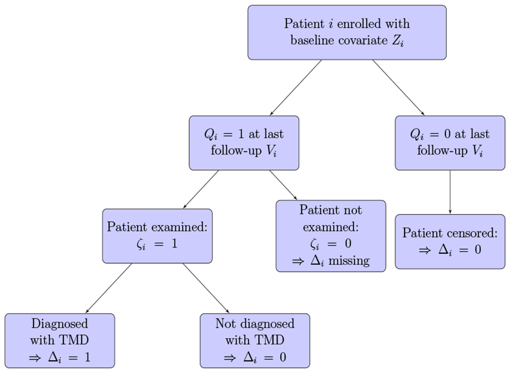
Study design flowchart: Patient i has been followed-up until V_i when the patient is either diagnosed with TMD or lost to follow-up, or the study ends. This figure appears in color in the electronic version of this article, and any mention of color refers to that version.

3.1. Shortcomings of Previous Methods

By the abuse of notation, P(W = w|E) given event E may denote the discrete conditional distribution when W is a discrete random variable, and may denote either the conditional density or the hazard function when W is a continuous random variable. When Q_i = 0, the subject is considered as non-informatively right-censored at V_i = v_i with likelihood contribution of P(T_i = v_i|Z_i). When Q_i = 1, we denote the risk P(C_i = t|V_i ≥ t; X_i) of non-informative censoring at time t as $\tilde{h}(t|{\mathit{X}}_i)$ where X_i is the vector of covariates associated with censoring time C_i. The usual assumption of non-informative missing mechanism (see Rubin 1976) for missingness indicator ζ_i implies that

$$P({\zeta }_i|V_i=t,{\mathit{X}}_i,{\mathit{Z}}_i,{\Delta }_i)=P({\zeta }_i|V_i=t,{\mathit{X}}_i,{\mathit{Z}}_i).$$ (6)

Using the usual assumption of non-informative censoring (Kalbfleisch and Prentice, 2002) at time V_i = t and the assumption of (6), we can show that

$$P({\Delta }_i=1|V_i=t,{\zeta }_i=0;{\mathit{Z}}_i,{\mathit{X}}_i)=\frac{\lambda (t|{\mathit{Z}}_i)}{\lambda (t|{\mathit{Z}}_i)+\stackrel{\sim }{h}(t|{\mathit{X}}_i)}.$$ (7)

The proof of (7) is in the Appendix.

Both the multiple imputation method from Brownstein et al. (2015) and the probability weighting method from Cook and Kosorok (2004) assume the logistic regression model

$$P({\Delta }_i=1|V_i=t,{\zeta }_i=0;{\mathit{Z}}_i,{\mathit{X}}_i)=\frac{\exp (\alpha {\mathit{X}}_i+\gamma {\mathit{Z}}_i+\eta t)}{1+\exp (\alpha {\mathit{X}}_i+\gamma {\mathit{Z}}_i+\eta t)},$$ (8)

while treating {V_i, Z_i, X_i} as predictors for the conditional distribution of Δ_i given ζ_i = 0. To ensure P(Δ_i = 1| V_i = t, ζ_i = 0; Z_i, X_i) in both (7) and (8) can be equal, additional restrictive assumptions must be made about the risk $\tilde{h}(t|{\mathit{X}}_i)$ of censoring and the hazard function λ(t|Z_i) in (1). For example, even when $\tilde{h}(t|{\mathit{X}}_i)$ follows the model $\tilde{h}(t|{\mathit{X}}_i)=h_0(t)\exp (-\gamma {\mathit{X}}_i)$ of Cox (1972), we need the highly restrictive assumption h₀(t)/λ₀(t) ∝ exp(−ηt) for some η > 0 to ensure the assumption of (8).

3.2. Bayesian Method

To overcome the need for additional restrictive assumptions about the relationship between h₀(t) and λ₀(t) as discussed in Section 3.1, we present a fully Bayesian method in which the likelihood function accommodates contributions from observations with missing censoring indicators. The censoring mechanism for a patient who did not screen positively (Q_i = 0) may be very different from a patient who did screen positively in questionnaires (Q_i = 1) and subsequently qualified for a dental examination at last observation time V_i. We do not consider modeling the censoring mechanism for a patient with Q_i = 0 because such a patient is always considered non-informatively censored at V_i with known Δ_i = 0, and we assume (reasonable for OPPERA study) that the censoring mechanism for the case Q_i = 0 is very different for the censoring mechanism for the case Q_i = 1. The likelihood contribution for such a patient will be

$$P(T_i>{\upsilon }_i|{\mathit{X}}_i,{\mathit{Z}}_i,Q_i=0)=P(T_i>{\upsilon }_i|{\mathit{Z}}_i)\propto \mathbf{\prod }_{j=1}^{m_i}\exp (-{\mu }_{ij}),$$ (9)

where v_i ∈ I_mi is the observed value of V_i, and μ_i1, ⋯, μ_imi are same as in (3). For a patient with Q_i = 1, we will need to model the censoring mechanism because the patient’s censoring indicator Δ_i may be unknown. For brevity of presentation, we will for the time being consider this censoring distribution to be piecewise exponential with corresponding hazard function $\tilde{h}(t|{\mathit{X}}_i)=h_j$ when t ∈ I_j. We can later allow this $\tilde{h}(t|{\mathit{X}}_i)$ to be more explicitly dependent on the vector X_i. For the case with {Q_i = 1, ζ_i = 1}, the likelihood contribution is

$$P(V_i\in [{\upsilon }_i,{\upsilon }_i+dt),{\Delta }_i|{\mathit{X}}_i,{\mathit{Z}}_i,Q_i=1)\simeq \{\mathbf{\prod }_{j=1}^{m_i}\exp (-{\mu }_{ij}-G_{ij})\}{({\lambda }_{m_i}{e}^{-{\mathit{\beta }}^{\prime }{\mathit{Z}}_i})}^{{\Delta }_i}{(h_{m_i})}^{1-{\Delta }_i}dt,,$$ (10)

where G_ij = h_jw_j for j < m_i, G_imi = h_mi(v_i − τ_mi−1). For the case with {Q_i = 1, ζ_i = 0}, the likelihood contribution is

$$P(V_i\in [{\upsilon }_i,{\upsilon }_i+dt)|{\mathit{X}}_i,{\mathit{Z}}_i,Q_i=1)\simeq \{\mathbf{\prod }_{j=1}^{m_i}\exp (-{\mu }_{ij}-G_{ij})\}({\lambda }_{m_i}{e}^{-{\mathit{\beta }}^{\prime }{\mathit{Z}}_i}+h_{m_i})dt.$$ (11)

The proofs of the equations (10) and (11) are in the Web-based Supplementary Materials. Based on the likelihood contributions in (9), (10) and (11), each subject’s likelihood contribution is proportional to one of four following cases.

Observation Cases	Likelihood Contribution
1. Qi = 0	$\exp (-{\sum }_{j=1}^{m_i}{\mu }_{ij})$
2. Qi = 1, ζi = 1, Δi = 0	$G_{i{m}_i}\exp (-{\sum }_{j=1}^{m_i}({\mu }_{ij}+G_{ij})\}$
3. Qi = 1, ζi = Δi = 1	${\mu }_{i{m}_i}\exp (-{\sum }_{j=1}^{m_i}({\mu }_{ij}+G_{ij})\}$
4. Qi = 1, ζi = 0	$(G_{i{m}_i}+{\mu }_{i{m}_i})\exp (-{\sum }_{j=1}^{m_i}({\mu }_{ij}+G_{ij})\}$

However, this likelihood L(β, λ₀, h|N, ζ, V, Z) obtained using above four cases is a nonstandard likelihood function that is not available in any standard statistical software. Therefore, to incorporate the likelihood L(β, λ₀, h|N, ζ, V, Z) within MCMC based software such as WinBUGS, OpenBUGS, Proc MCMC or JAGS, we use the fact that these above four cases of likelihood contributions are proportional to the likelihood contributions based on independent Poisson random variables D_1i ~ Poi(τ₁₁) and D_2i ~ Poi(τ_2i). As shown below, each (D_1i, D_2i) (except, only D_1i in case 1) is a function of the observed values of (V_i, Q_i, ζ_i, Δ_i) and corresponding (τ_1i, τ_2i) are following functions of the parameters (β, λ₀, h).

Observation cases	Data function	Poisson Parameters
1: Qi = 0	D1i = 0	${\tau }_{1i}={\sum }_{j=1}^{m_i}{\mu }_{ij}$
2: Qi = ζi = 1, Δi = 0	D1i = 0, D2i = 1	${\tau }_{1i}={\sum }_{j=1}^{m_i}{\mu }_{ij}+{\sum }_{j=1}^{m_i-1}{G}_{ij}$, τ2i = Gimi
3: Qi = ζi = Δi = 1	D1i = 0, D2i = 1	${\tau }_{1i}={\sum }_{j=1}^{m_i-1}{\mu }_{ij}+{\sum }_{j=1}^{m_i}{G}_{ij}$, τ2i = μimi
4: Qi = 1, ζi = 0	D1i = 0, D2i = 1	${\tau }_{1i}={\sum }_{j=1}^{m_i-1}({\mu }_{ij}+G_{ij})$, τ2i = Gimi + μimi

Because the product of Poisson likelihood contributions from each case with associated parameters (τ_1i.τ_2i) is proportional to the corresponding likelihood contribution of the observed data from subject i to the targeted likelihood L(β, λ₀, h|N, ζ, V, Z), we can obtain MCMC samples from the posterior p(β, λ₀, h|N, ζ, V, Z) via sampling from

$$p(\mathit{\beta },{\mathit{\lambda }}_0,\mathbf{h}|\mathbf{N},\zeta ,\mathbf{V},\mathbf{Z})\propto L(\mathit{\beta },{\mathit{\lambda }}_0,\mathbf{h}|\mathbf{D},\mathbf{Q},\zeta )\pi (\mathit{\beta },{\mathit{\lambda }}_0,\mathbf{h}),$$ (12)

where the likelihood L(β, λ₀, h|D, Q, ζ), the product of Poisson likelihood likelihood contributions based on set of observed indicators D = {D_1i, D_2i : i = 1, ⋯, n} and Q, can now be used in standard statistical software. Also, π(β, λ₀, h) in (12) is the joint prior distribution of (β, λ₀, h) based on the priors as defined in (5) and including the additional independent Gamma priors h_j ~ Gamma(1,1) for j = 1, …, J for the censoring risks (hazard rates of C_i) of patients with Q_i = 1.

4. Simulations

Using simulated data with missing-at-random (MAR) censoring indicators, we compare our Bayesian method with the “Multiple Imputation” method of Brownstein et al. (2015), the weighted samples method (called “Cook-Kosorok”) of Cook and Kosorok (2004), a Bayesian method under the ideal situation when all Δ_i are observed (called “No missing data”), as well as with following three ad hoc methods: (1) “Complete case only” method where a Bayesian analysis excludes all observations with missing Δ_i, (2) “Missing as censored” method where a Bayesian analysis treats all missing Δ_i as censored, (3) “Missing as failures” method where all missing Δ_i are treated as failures. Similar to the simulation studies in Brownstein et al. (2015), we perform our simulation studies with 3 different values of a single scalar regression parameter β ∈ {−0.5, −1.5, −3} of the proportional hazards model of (Cox, 1972) in Equation (1). For each of 3 simulation studies with different values of β, we generate n = 250 survival times T_i from model of (Cox, 1972) with baseline hazard λ₀(t) = 1 and mean 2 and unit variance normal distributed covariate Z_i. For each simulation model, the unknown sampling distribution of the estimator of the regression parameter β has been approximated (Monte Carlo) by using regression estimates from 250 datasets generated from the simulation model. Our aim is to compare these competing methods of estimation when the simulation model for missing mechanism for Δ_i follows the assumption of missing mechanism used in Brownstein et al. (2015). To achieve these purposes, we simulate non-informative random censoring times C_i using exponential distribution with mean 5, and we simulate Q_i = I(X_i > 0.5), where X_i has a normal density with mean V_i = min(T_i, C_i) and standard deviation 0.3. Thus, in our simulation model, Q_i depends on simulated V_i and X_i. To mimic the data generation mechanism of the OPPERA study as much as we reasonably can, we set the Δ_i to have no possibility of missing if Q_i = 0. This set-up is similar to the assumption of Bair et al. (2013) used for initial analysis of the data in the OPPERA study, such that Δ_i has the positive probability of missing only for subjects with Q_i = 1. However, our simulation model may generate observations with Q_i = 0 and Δ_i =1 (unlike in the OPPERA study where Q_i = 0 ⇒ Δ_i = 0). For observation with Q_i = 1 in our simulation model, we ensure that the probability of missing Δ_i follows the MAR assumption, (Rubin, 1976) because the missing indicators ζ_i are simulated with distribution

$$P({\zeta }_i=0|X_i,Z_i,V_i,Q_i=1)=\frac{\exp (-0.2-0.3Z_i+0.1V_i)}{1+\exp (-0.2-0.3Z_i+0.1V_i)},$$ (13)

that depends only on the covariates (X_i, Z_i) and the observation time V_i, but, is independent of Δ_i. Our simulation model results in a missing rate of approximately 50%, which is similar to the rate of missing censoring indicators in the OPPERA study (Bair et al., 2013).

In Table 1, the point estimates of β obtained from these six competing methods have been compared based on their sampling biases, square root of the mean square errors (MSE), and based on their interval coverage proportions and average interval widths. For analyses using both Cook and Kosorok’s weighted sample method and the multiple imputation method, the probability p_i = P(Δ_i = 1|ζ_i = 0, X_i, Z_i, V_i) of missing is based on a logistic regression model of (8) dependent on the covariates (X_i, Z_i) and the observed monitoring time V_i.

Table 1.

Simulation results: Monte Carlo approximations (based on 250 replicated data-sets with MAR censoring indicators) of sampling biases (Bias), and square-root of mean square errors ($\sqrt{MSE}$) of point estimates, and coverage probabilities and average widths of interval estimates from different competing methods

True β	Inference Method	Bias	$\sqrt{MSE}$	Width	Coverage
−0.5	No missing data	−0.0026	0.0416	0.1674	0.968
	Complete cases only	0.0023	0.0583	0.2163	0.960
	Missing as censored	0.1050	0.1206	0.2137	0.500
	Missing as failures	0.0002	0.0423	0.1706	0.980
	Cook-Kosorok	−0.0024	0.0431	0.1744	0.964
	Multiple Imputation	0.0409	0.0619	0.2007	0.900
	Fully Bayesian	−0.0155	0.0199	0.2800	0.996
−1.5	No missing data	−0.0036	0.0815	0.3181	0.952
	Complete cases only	−0.0631	0.1252	0.4315	0.932
	Missing as censored	0.1212	0.1567	0.4210	0.828
	Missing as failures	0.0627	0.1029	0.3160	0.868
	Cook-Kosorok	−0.0055	0.0847	0.3397	0.952
	Multiple Imputation	0.0834	0.1170	0.3877	0.908
	Fully Bayesian	−0.0621	0.0624	0.5640	1.000
−3	No missing data	−0.0119	0.1943	0.7553	0.952
	Complete cases only	−0.2077	0.3575	1.0893	0.900
	Missing as censored	0.1034	0.3017	1.0406	0.920
	Missing as failures	0.5900	0.6196	0.6283	0.092
	Cook-Kosorok	−0.0230	0.2105	0.9013	0.964
	Multiple Imputation	0.4473	0.4877	0.9369	0.508
	Fully Bayesian	−0.3504	0.3505	1.4043	1.000

Width: Average of the widths of 250 interval estimates of β.

Coverage: Proportion of times 250 interval estimates contain true β.

To obtain estimates of β using Cook-Kosorok method, we estimate the probability p_i for each subject with ζ_i = 0 via the frequentist logistic regression analysis based on the model in (8). Then, we fit a proportional hazards model to the data set after replacing each observation with missing Δ_i with two new weighted observations with identical (Z_i, V_i), but different Δ with corresponding weights. The first new observation has Δ = 1 and weight $\widehat{p_i}$, and the second observation has Δ = 0 and weight $1-\widehat{p_i}$. Finally, we record the estimated regression coefficient, $\widehat{\beta }$. For the Cook-Kosorok method, we use 1,000 bootstrap replicates to estimate the variance of $\widehat{\beta }$ and to construct 95% bootstrap percentile interval (β_0.025, β_0.0975) for β. Similarly, for the multiple imputation method, the coefficients (α, γ, η) of the logistic regression model for p_i in (8) are estimated based on data from subjects with observed Δ_i values and using a Bayesian method with all 3 coefficients having independent Cauchy(0, 2.5) priors. Ten sets of multiple imputations of missing Δ_i are then generated such that $P({\Delta }_i=1|{\zeta }_i=0)=\widehat{p_i}$ and used to estimate β.

MCMC samples for all Bayesian methods are obtained using JAGS software. Remaining code parallels the corresponding items in Brownstein et al. (2015). Briefly, the following main functions are used. Bootstrap estimates of the standard error of $\widehat{\beta }$ of Cook and Kosorok are obtained using the boot and boot.ci functions within the boot R package (Canty and Ripley, 2016). The mi.binary function of the mi R package (Gelman and Hill, 2011) is used to generate imputed values of the missing Δ_i for the multiple imputation method. Cox’s (1972) models are fit using the survfit function in the survival R package (Therneau, 2015).

Estimates from our fully Bayesian method, the multiple imputation method and the Cook-Kosorok method generally have reasonably low sampling bias and high coverage. Unsurprisingly, the estimates produced by the three ad hoc methods tend to have larger biases compared to other methods. Coverage for our Bayesian method reached or exceeded the nominal level. By comparison, the ad-hoc methods and multiple imputation had inadequate coverage proportions. Meanwhile, our Bayesian method produces estimates with reasonable MSE, especially compared to the ad-hoc methods and the multiple imputation method. In addition, in two scenarios, our fully Bayesian method produced the smallest mean squared error (MSE) for $\widehat{\beta }$. Only the method by Cook and Kosorok (2004) had comparable results. These findings suggest that our fully Bayesian method produces interval estimates with high coverage without markedly sacrificing MSE and outperforms most competing methods. By contrast, the multiple imputation method yields poor coverage proportions (especially as the true β value increases). This suggests that multiple imputation method (on average) underestimates the sampling variability of the estimated β. In contrast, we found that the $\sqrt{MSE}$ for the fully Bayesian method is approximately equal to or less than the average posterior standard error estimate (not-shown, for conciseness) in all three scenarios. For the purpose of investigating the effects of priors on Bayesian estimates, we have used a standard normal prior density on β centered at 0, and this prior on β is substantially biased when true β has large magnitude. However, our results in Table 1 show very moderate effects of this prior on the interval and point estimates of β. For example, the width of Bayesian interval estimate is only 40% bigger than the width of the interval estimate from Cook-Kosorok method when true β = −3 is very different from the prior (less than 0.2% prior probability of {β < −3}).

In summary, the Bayesian methods performed well in these simulations by exhibiting high coverage and maintaining MSE values comparable to most other methods. By design, the simulation parameters actually follow the restrictive assumptions used by Cook-Kosorok and multiple imputation and discussed in Section 3.1. In scenarios when the restrictive assumptions are violated, competing methods, such as multiple imputation and Cook-Kosorok, would be expected to exhibit worse performance, while the Bayesian method performance would likely remain unchanged. Thus, this simulation study was designed more of a study of the “robustness” of our new Bayesian method compared to existing methods under the best possible conditions for the existing methods.

5. Analysis of the OPPERA Study

The Orofacial Pain: Prospective Evaluation and Risk Assessment (OPPERA) is a large prospective cohort study designed to identify risk factors for first-onset temporomandibular disorder (TMD). Between 2006 and 2008, 3,263 subjects without TMD were recruited at four study sites. After enrollment, each subject was evaluated for possible risk factors of TMD. Thereafter, he/she was asked to complete a quarterly questionnaire to evaluate whether he/she had some possibility to develop TMD since their previous questionnaire. Subjects who screened positively based on their questionnaire were slated to receive a follow-up invasive dental examination by a clinical expert to diagnose the presence or absence of TMD. Unfortunately, some of these subjects screening positively missed the follow-up dental examination and thus had missing censoring indicators. Previously, Bair et al. (2013) examined univariate relationships between attendance at the clinical examinations and possible predictor variables and found a few statistically significant differences between examined and non-examined subjects, indicating that the censoring indicators are not MCAR. For a more detailed description of the OPPERA study, methodology, and initial findings, see Maixner et al. (2011), Slade et al. (2011), and Bair et al. (2013).

A small number of subjects in the OPPERA study had multiple dental examinations because their previous dental examinations had resulted in non-diagnosis of TMD, and they subsequently screened positively again. In the present as well as previous analyses only the most recent questionnaire and resulting TMD diagnosis (or missing Δ) were used. Thus, each subject had at most one positive screening result and possibility to have TMD diagnosis only at last minitoring time. As reported by Bair et al. (2013), dental examinations performed by one examiner resulted in a much higher percentage of subjects diagnosed with TMD compared to the other examiners. We also omit all of the clinical examinations by this examiner from our analysis and instead consider them as missing.

To compare our method Bayesian analysis of the OPPERA data with analysis using existing methods for missing failure indicators, we analyze the regression effects of the same subset of risk factors for TMD used in Brownstein et al. (2015), namely a collection of clinical, psychosocial, and quantitative sensory testing items. For the analysis in this and previous papers, the clinical variables are categorical, and the quantitative sensory testing and psychosocial variables are continuous. Continuous variables have been all standardized to have zero mean and unit standard deviation. There are no missing predictor variables because the few missing values in these predictor variables were previously imputed once per missing observation via the expectation-maximization (EM) algorithm, as described in Greenspan et al. (2011) and Fillingim et al. (2011).

The Bayesian analysis of the data treating all missing indicators as censored and our fully Bayesian method were run with 2 chains of 1500 burn-in iterations and 5000 iterations. (Note: Three models took longer to converge, these were run with 2 chains of 45,000 burn-in iterations and 5000 additional iterations.) In all runs, computed in JAGS software, fifteen equally spaced grid intervals were used. Convergence and auto-correlation for all models were checked using diagnostic plots. The Bayesian p-values for the OPPERA analysis are calculated per Lin et al. (2017) as 2 × min{P(θ > 0|Data), P(θ < 0|Data)}.

In Table 2, we only compare the results of our Bayesian analysis to the multiple imputation method of Brownstein et al. (2015) and to the naive method of considering all missing censoring indicators as censored. (We do not present the comparison with Cook and Kosorok (2004), because it has been already been shown to be markedly worse than Brownstein et al. (2015) in terms of computational feasibility.) To align our Bayesian analysis with the multiple imputation method based analysis as in Brownstein et al. (2015), all of our Cox’s regression models adjust for the effects of the count of non-specific orofacial symptoms and OPPERA study site.

Table 2.

Results from the Orofacial Pain: Prospective Evaluation and Risk Assessment.

	Treat Missing as Censored				Multiple Imputation				Fully Bayesian
	HR	LCL	UCL	P	HR	LCL	UCL	P	HR	LCL	UCL	P
Clinical Variable
Mouth	3.26	1.83	5.84	<0.001	2.47	1.43	4.25	0.001	3.24	1.95	4.85	0.002
Chronic Pain Disorders	3.08	2.26	4.21	<0.001	2.36	1.79	3.11	<0.001	3.09	2.40	3.88	<0.001
Respiratory Conditions	1.38	1.01	1.87	0.041	1.42	1.11	1.83	0.006	1.24	0.96	1.55	0.072
Smoking: current	1.26	0.86	1.84	0.240	1.40	0.97	2.03	0.073	1.56	1.13	2.06	0.005
Smoking: former	1.87	1.22	2.87	0.004	1.65	1.10	2.48	0.017	1.62	1.11	2.20	0.043
Right Temporalis	1.83	1.32	2.52	<0.001	1.55	1.19	2.02	0.001	1.72	1.32	2.19	<0.001
Left Temporalis	1.60	1.14	2.25	0.006	1.45	1.06	1.99	0.021	1.57	1.18	2.04	0.004
Right Masseter	1.85	1.35	2.53	<0.001	1.67	1.28	2.19	<0.001	1.74	1.35	2.20	<0.001
Left Masseter	1.70	1.23	2.35	0.001	1.52	1.14	2.03	0.004	1.63	1.25	2.08	0.003
Psychosocial variable
PILL Global Score	1.52	1.35	1.71	<0.001	1.43	1.29	1.60	<0.001	1.43	1.31	1.57	<0.001
EPQ-R Neuroticism	1.39	1.21	1.60	<0.001	1.25	1.10	1.42	0.001	1.34	1.19	1.50	<0.001
Trait Anxiety Inventory	1.43	1.25	1.64	<0.001	1.34	1.18	1.52	<0.001	1.39	1.25	1.54	<0.001
Perceived Stress Scale	1.35	1.17	1.55	<0.001	1.29	1.15	1.46	<0.001	1.36	1.22	1.51	<0.001
SCL 90R Somatization	1.44	1.31	1.58	<0.001	1.40	1.30	1.52	<0.001	1.45	1.35	1.55	<0.001
QST variable
Pressure: temporalis	1.26	1.07	1.49	0.007	1.17	1.00	1.37	0.046	1.20	1.06	1.36	< 0.001
Pressure: masseter	1.23	1.04	1.45	0.017	1.14	0.98	1.33	0.082	1.21	1.05	1.37	0.008
Pressure: TM joint	1.25	1.05	1.48	0.011	1.16	1.02	1.32	0.027	1.22	1.08	1.38	0.003
Mechanical pain, 15s:	1.23	1.09	1.38	0.001	1.17	1.05	1.30	0.004	1.22	1.10	1.33	< 0.001
Mechanical pain, 30s:	1.20	1.07	1.34	0.002	1.14	1.02	1.27	0.026	1.19	1.08	1.30	< 0.001

HR: hazard ratio; LCL: lower limit of 95% interval estimate; UCL: upper limit of 95% interval estimate; P: p-value; QST: Quantitative sensory testing; TM: temporomandibular; PILL: Pennebaker Inventory of Limbic Languidness; EPQ: Eysenck Personality Questionnaire; SCLR-90R: Symptom Checklist-90, Revised.

Results in Table 2 show a mixture of effects that are sensitive to the analysis method and effects that are qualitatively similar for the three methods. We begin by highlighting some of the effects that differ based on analysis method. A naive analysis treating all missing indicators as censored does not detect a statistically significant association at the traditional 5% level of being a “current smoker” (as opposed to a “never smoker”) with the time to first-onset TMD (HR=1.26, p=0.24). However, more substantial evidence for this association is apparent while using our fully Bayesian approach, with a larger hazard ratio and markedly smaller p-value (HR=1.56, p=0.005). Under multiple imputation, the association is less clear, where the multiple-imputation point estimate of the hazard ratio of first-onset TMD for a current smoker compared to a never smoker is smaller than the point estimate for the Bayesian method, and the multiple imputation p-value is higher at 0.073. (In Brownstein et al. 2015, the multiple imputation point estimate was similar in magnitude, but the p-value was smaller, at 0.0166.) In other words, the observed effect of smoking on TMD was stronger under the Bayesian method than if the missing data was treated as censored or if multiple imputation was used. On the other hand, the point estimator of the hazard ratio of first-onset TMD for a former smoker is smaller when using the Bayesian approach compared to methods based on treating missing as censored and multiple imputation. In other words, using the Bayesian method yielded a stronger effect for former smokers and weaker effect for current smokers, both compared to never smokers. As another example, the estimated hazard ratio for the history of five respiratory conditions is noticeably smaller in Bayesian analysis compared to under other methods, and, unlike the other two methods, the Bayesian credible interval contains the null value of unity, which corresponds to the lack of data-evidence for an association between having a history of five respiratory conditions and risk of first-onset TMD.

All psychosocial variables listed in Table 2 were significant after applying the fully Bayesian method, which was consistent with the methods compared. Hazard ratios for all psychosocial variables were similar or slightly higher after applying the fully Bayesian method, as compared to multiple imputation. Bayesian credible intervals were narrower than or comparable to corresponding intervals for other methods.

A similar effect was seen in the Quantitative Sensory Testing (QST) variables. Of particular interest, Brownstein et al. (2015) found that the three variables related to pressure pain threshold became weakly (or not) associated with first-onset TMD after applying their multiple imputation method, as compared to the ad hoc method of treating all missing censoring indicators as censored. After implementing the fully Bayesian method, we found that the pressure pain threshold variables for temporalis, masseter, and TM joint all have hazard ratios and credible intervals in support of hypotheses of associations with first-onset TMD.

For the first time for missing censoring indicators, we present diagnostic plots to evaluate how Cox's model assumption holds for the OPPERA study. Specifically, our diagnostic plots are based on $-\log [\widehat{S}\{\widehat{{\Lambda }_i}(V_i)\}]$ versus $\widehat{{\Lambda }_i}(V_i)$, where $\widehat{{\Lambda }_i}(V_i)$ is the posterior estimate of exp(βZ_i)Λ₀(V_i) and $\widehat{S}\{\widehat{{\Lambda }_i}(V_i)\}$ is the Kaplan-Meier estimator obtained from $\{\widehat{{\Lambda }_i}(V_i),{\Delta }_i\}$ for i = 1, ⋯, n. Under the case of no missing Δ_i we expect this plot to be close to a straight line with slope one when the model is correct because $\{\widehat{{\Lambda }_i}(V_i),{\Delta }_i\}$ is a censored sample from an exponential distribution with mean 1 if Cox’s model assumption is correct. To accommodate the subjects with missing Δ_i we will replace each missing subject with missing Δ_i with one subject with weight w_i and $\{\widehat{{\Lambda }_i}(V_i),\Delta =0\}$ and another with weight $(1-w_i)$ (1−w_i) and $\{\widehat{{\Lambda }_i}(V_i),\Delta =1\}$, where w_i is the posterior estimate of h_imi/{h_mi + λm_i exp(−βZ_i)} (probability of getting censored given at risk in the interval of last observation time). Using this idea of weighted observations replacing each observation with missing Δ_i we also develop and present the plots of martingale residuals versus some specific covariates. For the brevity of presentation of our analysis, in Figure 2 we only show two plots for the most important clinical predictors. These and other plots conclude that the Cox’s modeling assumption is reasonably appropriate for the OPPERA data study.

Figure 2.

Diagnostic plots for Bayesian analysis of the OPPERA study: figure (a) is a plot of $-\log [\widehat{S}\{\widehat{\Lambda }(V_i)\}]$ versus $\widehat{\Lambda }(V_i)$ for one binary clinical covariate, chronic pain. Figure (b) is the martingale residual versus covariate plot for chronic pain. This figure appears in color in the electronic version of this article, and any mention of color refers to that version.

6. Discussion

We have developed a fully Bayesian method for the analysis of time-to-event data with missing censoring indicators. Our method can be implemented using readily available software such as WinBUGS, Proc MCMC, or JAGS. The ability to use these standard software packages is highly attractive given both the reliability and available tools (such as convergence diagnostics) that these existing software programs provide. A valid method for handling data with missing censoring indicators is crucial in studies where failure status is not instantaneously recorded. This study framework may lead to missing failure indicators and is common for diseases, such as TMD, that are involve challenging or costly diagnostic procedures.

Our method requires that the missing data be, at minimum, MAR. Bair et al. (2013) searched for differences between subjects who did attend their clinical examinations versus those who did not, with respect to both demographic variables and risk factors for TMD measured by the questionnaire and found very few associations. In each simulation scenario under the MAR assumption, our method produced no significant bias, as well as the either the narrowest or very close to the narrowest credible interval. When using a fully Bayesian method, the average posterior variance of the estimated regression coefficient is slightly greater than or approximately equal to the mean squared error, showing that the proposed method does not underestimate the variance of the regression coefficient.

When applying our method to the OPPERA data, it is evident that some of the hazard ratios and interval estimates associated with some variables were noticeably different than the corresponding estimates after using multiple imputation or treating all missing censoring indicators as censored. Precise calculation of the hazard ratios associated with putative risk factors for TMD is important, as the results of OPPERA are already well-cited and may influence future dental pain literature and standardize orofacial care. Therefore, we suggest that estimation of the regression parameters in a Cox model in the presence of missing failure indicators is done via a fully Bayesian model.

References

- Bair E, Brownstein NC, Ohrbach R, Greenspan JD, Dubner R, Fillingim RB, et al. (2013). Study protocol, sample characteristics, and loss to follow-up: The oppera prospective cohort study. The Journal of Pain 14, T2–19. [DOI] [PMC free article] [PubMed] [Google Scholar]
- Brownstein N, Cai J, Slade G, and Bair E (2015). Parameter estimation in cox models with missing failure indicators and the oppera study. Statistics in Medicine 34, 3984–3996. [DOI] [PMC free article] [PubMed] [Google Scholar]
- Canty A and Ripley B (2016). boot: Bootstrap R (S-Plus) Functions. R package version 1.3-18. [Google Scholar]
- Cook TD and Kosorok MR (2004). Analysis of time-to-event data with incomplete event adjudication. Journal of the American Statistical Association 99, 1140–1152. [Google Scholar]
- Cox D (1972). Regression models and life-tables. Journal of the Royal Statistical Society. Series B (Methodological) 34, 187–220. [Google Scholar]
- Fillingim RB, Ohrbach R, Greenspan JD, Knott C, Dubner R, Bair E, Baraian C, Slade GD, and Maixner W (2011). Potential psychosocial risk factors for chronic tmd: descriptive data and empirically identified domains from the oppera case-control study. The Journal of Pain 12, T46–T60. [DOI] [PMC free article] [PubMed] [Google Scholar]
- Gelman A and Hill J (2011). Opening windows to the black box. Journal of Statistical Software 40,. R package version 9.15. [Google Scholar]
- Greenspan JD, Slade GD, Bair E, Dubner R, Fillingim RB, Ohrbach R, Knott C, Mulkey F, Rothwell R, and Maixner W (2011). Pain sensitivity risk factors for chronic tmd: descriptive data and empirically identified domains from the oppera case control study. The Journal of Pain 12, T61–T74. [DOI] [PMC free article] [PubMed] [Google Scholar]
- Ibrahim JG, Chen M-H, and Sinha D (2001). Bayesian Survival Analysis. Springer, New York. [Google Scholar]
- Kalbfleisch JD and Prentice RL (2002). The Statistical Analysis of Failure Time Data. Wiley, New York. [Google Scholar]
- Lin Y, Lipsitz SR, Sinha D, Fitzmaurice G, and Lipshultz S (2017). Exact bayesian p-values for a test of independence in a 2 x 2 contingency table with missing data. Statistical Methods in Medical Research. [DOI] [PMC free article] [PubMed] [Google Scholar]
- Maixner W, Diatchenko L, Dubner R, Fillingim RB, Greenspan JD, Knott C, et al. (2011). Orofacial pain prospective evaluation and risk assessment study – the oppera study. The Journal of Pain 12, T4–11. [DOI] [PMC free article] [PubMed] [Google Scholar]
- Rubin DB (1976). Inference and missing data. Biometrika 63, 581–592. [Google Scholar]
- Slade GD, Bair E, By K, Mulkey F, Baraian C, Rothwell R, et al. (2011). Study methods, recruitment, sociodemographic findings, and demographic representativeness in the oppera study. The Journal of Pain 12, T12–T26. [DOI] [PMC free article] [PubMed] [Google Scholar]
- Slade GD, Fillingim RB, Sanders AE, Bair E, Greenspan JD, Ohrbach R, Dubner R, Diatchenko L, Smith SB, Knott C, et al. (2013). Summary of findings from the oppera prospective cohort study of incidence of first-onset temporomandibular disorder: implications and future directions. The Journal of Pain 14, T116–T124. [DOI] [PMC free article] [PubMed] [Google Scholar]
- Therneau T (2015). A Package for Survival Analysis in S. R package version 2.38. [Google Scholar]
Associated Data
This section collects any data citations, data availability statements, or supplementary materials included in this article.