

Abstract
Precomputed affinity maps are used by AutoDock to efficiently describe rigid biomolecules called receptors in automated docking. These maps greatly speed up the docking process and allow users to experiment with the forcefield. Here we present AutoGridFR (AGFR): a software tool facilitating the calculation of these maps. We describe a new version of the AutoSite algorithm that improves the description of binding pockets automatically detected on receptors, and an algorithm for adding affinity gradients which help search methods optimize solution using fewer evaluations of the scoring functions. AGFR supports the calculation of maps for various advanced docking techniques such as covalent docking, hydrated docking, and docking with flexible receptor sidechains. Maps are stored in a single file along with metadata supporting data provenance, reproducibility, and facilitating their management. Finally, maps can be calculated from the command line or through a modern graphical user interface which also supports their visualization.
Keywords: Affinity maps, docking, covalent docking, docking with flexible receptor sidechains, provenance
Introduction
Over the past 20 years, the automated ligand-receptor docking software program AutoDock1 has gathered a large community of users and has become the most cited docking software2. AutoDock represents the rigid part of the receptor using 3D rectilinear grids called affinity maps and computed by AutoGrid1. For a given receptor and a docking box, an affinity map is computed for each atom type present in the ligand to be docked, along with electrostatic and desolvation maps. These maps greatly reduce docking calculation runtimes as they allow the calculation of interactions between a ligand atom and the entire set of atoms in the receptor using trilinear interpolations in the maps. While it is possible to compute these maps on the fly, as is done in AutoDock Vina3, precomputing them presents several interesting advantages. Custom water maps4 have been used to perform hydrated docking5, where water mediated interactions between ligands and receptor are predicted as part of docking a ligand. Attractors maps have been used to study covalent docking6 and to dock ligands with flexible macrocycles7. These maps are also used by binding pocket prediction algorithms, such as AutoLigand8 and AutoSite9. Their visual inspection can provide useful insights into binding modes and ligand optimizations. Finally, in virtual screening applications, where millions of ligands are docked against the same receptors in parallel, precomputing affinity maps prevents recomputing them for each ligand docked.
Software tools, including those previously developed by us, provide only basic support for positioning and computing these affinity maps1,10,11,12, mostly allowing for the visual placement and scaling of the docking box. Moreover, they are relying on aging graphical toolkits. These reasons motivated the development of a new software tool: AutoGridFR or AGFR in short. The software was designed to: i) provide a range of common options for positioning and sizing the docking box and the parameters involved in the calculation of the maps; ii) allow the calculation of maps from a Command Line Interface (CLI) or using a modern graphical user interface (GUI); iii) incorporate our latest algorithms for identifying pockets and for post-processing maps; iv) support the creation of maps for advances docking applications such as covalent docking, hydrated docking, docking with flexible side chains, or creating maps for multiples binding sites; and v) facilitate map management and support data-provenance and reproducibility through the addition of meta data. For the latter, we designed a file container (target file), which stores the affinity maps calculated by AutoGrid, along with metadata about the maps and their creation. The maps stored in target files are backwards compatible with AutoDock4.
In this paper, we describe our new software tool AGFR for specifying, computing, visualizing and analyzing AutoDock Affinity maps saved as target files which facilitate their management. AGFR retains all the advantages of precomputed affinity maps while reducing the complexity of creating and managing these maps.
Methods
In this section, we first describe a post-processing algorithm available in AGFR for creating an affinity gradient that facilitates resolving ligand receptor clashes during docking. We also describe an algorithm for processing binding pockets identified by AutoSite in order to obtain better binding pocket descriptions. Finally, we provide a short description of the AGFR functionality and its GUI.
Receptor gradient
In the affinity maps calculated by AutoGrid4, the regions covered by the receptor contain high frequency values ranging from small negative (i.e., favorable affinity regions) to large positive values (i.e. inside the receptor core). The presence of numerous local minima in between receptor atoms (Fig 1, left panel) can hinder the optimization of a ligand that overlaps with the receptor, which happens frequently during the early stage of the automated docking process. We defined and implemented a protocol to replace these high frequency values inside the receptor by a gradient from the inside of the receptor toward its surface (Fig. 1, right panel). The gradient guides ligands overlapping with the receptor toward its surface. The gradient is calculated for all maps except the electrostatic and desolvation maps. Map values are only modified in regions inside the receptor, thus docked ligands that do not overlap with the receptor yield identical score with maps with gradients and with the original maps. The process for adding gradients is parallelized using OpenMP13.
Figure 1:
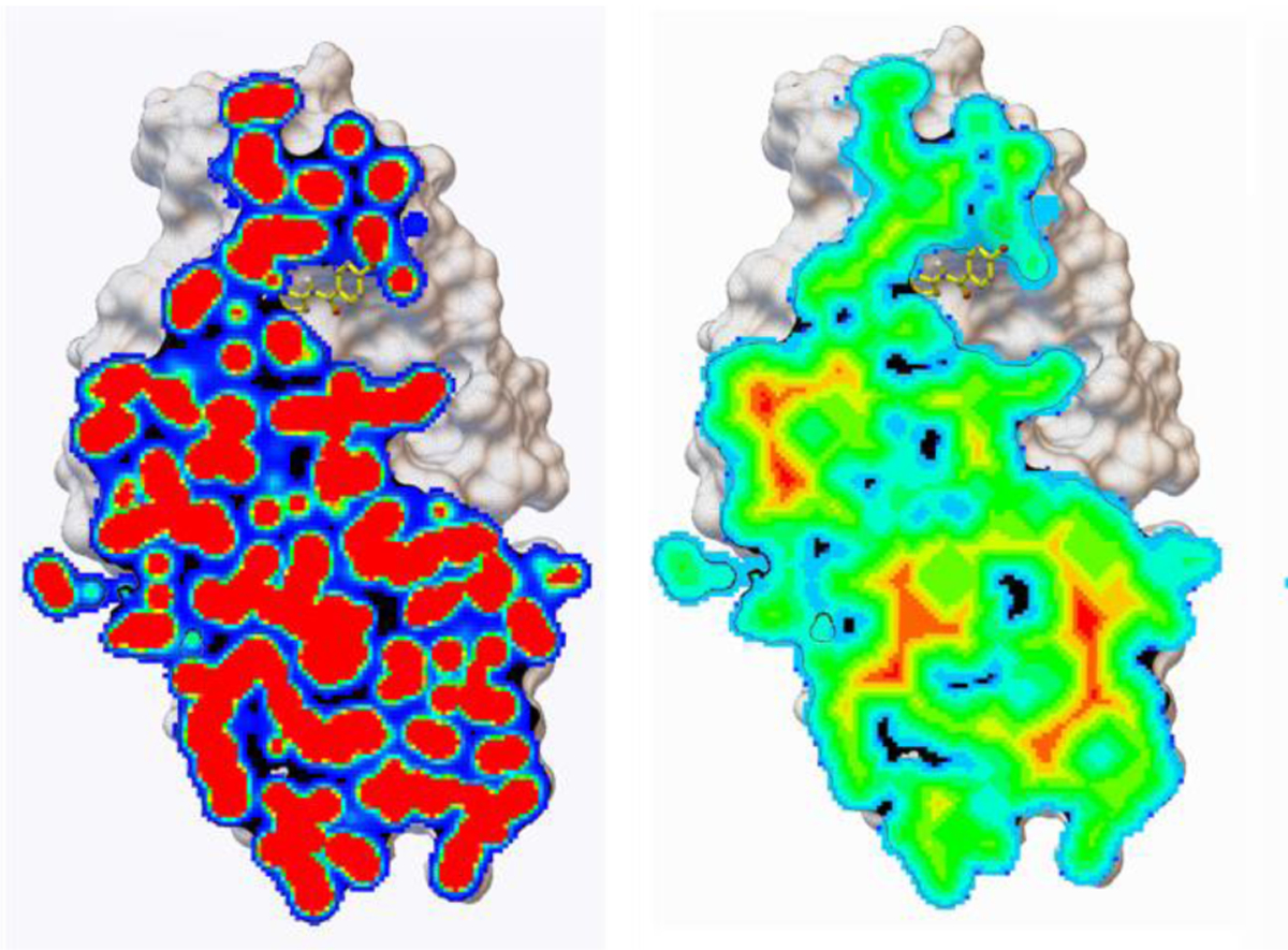
carbon affinity map cross sections. One the left a cross section of the original carbon affinity map of 4EK3 limited to the interior of the protein. On the right, the same cross section after adding the gradient. This Figure was created with PMV v 1.5.714,15
To assess the impact of these gradients on optimizing ligands during docking, we selected 4 ligand-receptor complexes with varying search complexity (i.e. numbers of rotatable bonds, receptor pocket shapes). We then compared the ability of the Solis-Wets local search algorithm16 (SW) implemented in AutoDockFR to optimize ligands in a typical docking scenario. Given the stochastic nature of SW and to avoid bias from the starting ligand poses, we generated 500 populations of 100 random initial docking poses, simulating the initial stage of 500 docking experiments for each of the complexes. We then minimized each pose using the SW local search. Briefly, SW stochastically creates small perturbations to the pose’s orientation and conformation, looking for perturbations that improve the score. Each perturbation is a set in SW and requires evaluating the scoring function for the perturbed solution. The algorithm stops when it reaches the maximum number of steps, or if it fails to improve the score after several consecutive steps. For each population we kept track of the averages of the following 4 metrics: 1) the number of ligand-receptor clashes, i.e. ligand-receptors heavy atoms located within a distance smaller than the sum of their van der Waals radii.; 2) the number of poses reaching a negative energy; 3) the number of evaluations of the scoring function used up by the SW procedure; and 4) the Root Mean Square Deviation (RMSD) between the starting and the minimized poses. We calculated the mean values of these metrics over the 500 populations and the differences of means values obtained with the original maps and the maps with gradients are reported in Table 1.
Table 1:
improved minimization performances. Differences in mean values calculated over 500 populations of 100 individuals for 4 metrics: the number of clashes, the number of poses with negative energy, the number of steps taken by the SW algorithm before giving up, the RMSD between the initial and the randomized pose.
| Differences in mean values (with Gradients – without Gradients) |
|||||
|---|---|---|---|---|---|
| PDB | #torsions | #clashes | #negative | #steps | RMSD |
| 1ac8 | 0 | −7.4 | 10.1 | 5.6 | 0.4 |
| 1kzk | 11 | −40.3 | 1.3 | 23.2 | 1.6 |
| 7cpa | 17 | −42.6 | 15.3 | 32.3 | 2.2 |
| 2vaa | 32 | −39.4 | 0.88 | 22.3 | 1.9 |
Table 1 shows that adding gradients to the maps uniformly improves these metrics, consistently reducing the average number of clashes, increasing the average number of poses reaching a negative energy, increasing the number of steps (e.g. reducing the number of time SW fails to identify a perturbation that improves the score), and increasing the average RMSD between the initial pose and the minimized pose. The Differences in mean values reported in Table 1 are significant with a 95% confidence interval based on the bootstrap method, confirming that the affinity gradients added to the maps significantly helps SW optimize poses.
AutoSite 1.1
AutoSite 1.0 uses affinity points from the carbon, oxygen and hydrogen affinity maps to identify potential binding pockets on a biological macromolecule. These pockets are modelled as clusters of contiguous grid points from the affinity maps called “fills”. Version 1.0 uses a single cutoff value per map to select high affinity points. Version 1.1 improves upon the original implementation by scanning these cutoff values around their values is in the original algorithm. As the cutoff values are relaxed, fills merge describing larger pockets. This information is stored in a hierarchical data structure which can be used to instantly identify pockets suitable for a given ligand, based on its size.
Version 1.1 also introduces two post-processing steps that lead to better binding pocket descriptors (Figure 2). The pocket descriptions calculated by AutoSite 1.0 rely solely on high affinity points, and thus, mostly captures the parts of the binding site occupied by ligand atoms that interact with the receptor. Ligand scaffolding atoms can have little to no interactions with the receptor and are therefore not well covered by these fills. We developed an automatic inflation procedure that extends fills toward the cavity opening, resulting in fills that better cover scaffolding ligand atoms, and thus improving the coverage of the volume occupied by known bound ligands. During docking, the ligand’s position relative to the receptor is defined by a translation which points from a central point in the ligand (called the root) to a position in the docking box. Reasonable end points for this vector are such that the ligand is not buried deeply inside the receptor or located too far from it to interact. Such a set of points can be specified in the target file and will be used by AutoDockFR17 and AutoDock CrankPep18 to sample the position of the ligand more efficiently during docking. The points from the fills identified by AutoSite 1.0 offer a reasonable set of such points. In version 1.1 we added a deflation procedure that shrinks the inflated fills described above by removing layers of points iteratively, until only 1/5 of the original volume remains. This procedure generates better sets of points for translation the ligand.
Figure 2.
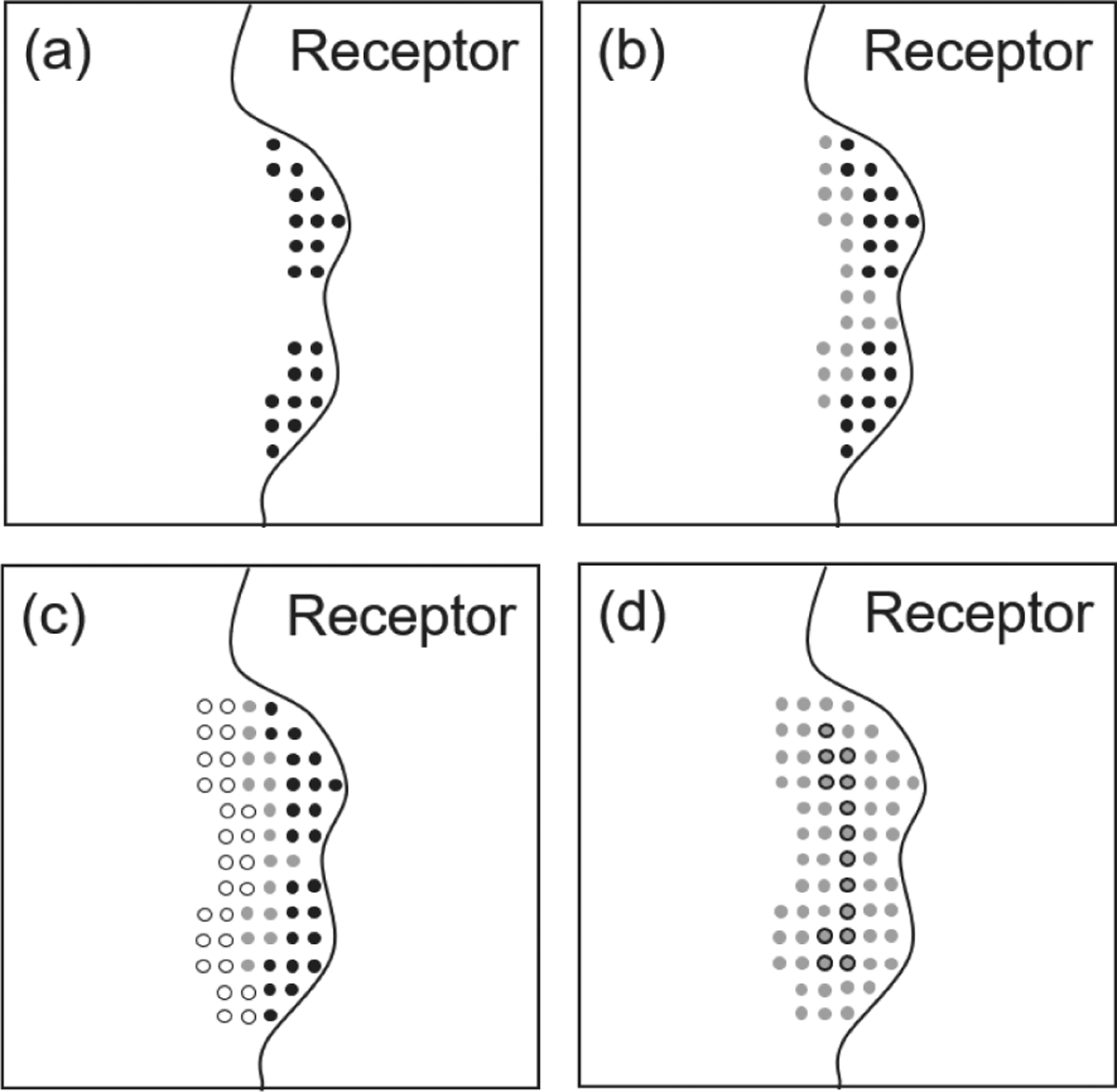
Algorithm overview for AutoSite 1.1. (a) The black dots show pockets (called fills) detected by the original AutoSite algorithm; (b) in version 1.1, as cutoffs for high affinity points are relaxed, grey points are added to the fills causing some of them to merge creating larger fills suitable for larger ligands; (c) Post-processing 1: a fill, selected as the pocket representation for a given ligand, is inflated by including points surrounding the fill, excluding points located between the cluster and the receptor (white circles). This description provides better overlap with known ligands; (d) Post-processing 2: a better set of points for placing the ligand in the pocket during docking (grey with black outline) is obtained by deflating (i.e. removing outer layers of points shown in grey) until only one 5th of the points remain.
We compared the fills produced by version 1.0 and 1.1 of AutoSite on the following two data sets. The Astex Diverse Set19 is comprised of 85 small molecule-protein complexes. This data set was used for the calibration of AutoSite 1.0. The LEADS-PEP dataset20 is comprised of 53 peptide-protein complexes. As in the original AutoSite publication, the quality of the fills was assessed using the Jaccard coefficient21 (JC), which measures how well two volumes overlap and is defined as follows. For two volumetric regions of space, R1 (i.e. the known ligand) and R2 (i.e. the AutoSite fill) this coefficient is defined as the ratio of the volume of the intersection of R1 and R2 divided by the volume of the union of R1 and R2. A perfect value of 1.0 is achieved by a fill that entirely covers the ligand, without extending into regions not covered by the ligand. Fills with JC ≥ 0.2 are typically considered acceptable.
Despite the fact that AutoSite 1.0 was calibrated on the Astex Diverse Set, Table 2 shows that version 1.1 still marginally improves the JC for this set. However, on the LEADS-PEP dataset the improvement is dramatic and moves the JC into the acceptable range.
Table 2.
Comparisons of Averaged Jaccard coefficients for LEADS-PEP and Astex Diverse set binding pockets.
| AutoSite version | Astex | LEADS-PEP |
|---|---|---|
| 1.0 | 0.339 | 0.143 |
| 1.1 | 0.362 | 0.234 |
Table 3 shows that the deflation algorithm implemented in AutoSite 1.1 produces fewer translation points for placing the ligand into the pocket during docking.
Table 3.
Comparison of the number of ligand translation points obtained with AutoSite 1.0 and AutoSite 1.1.
| AutoSite version | Average number of translation points | |
|---|---|---|
| Astex | LEADS-PEP | |
| 1.0 | 259.9 | 213.9 |
| 1.1 | 75.8 | 130.6 |
Moreover, this smaller set of points more often contains a point located within 2 Å of the crystallographic position of the ligand root (Table 4). Using the set of points increasing the chances to assign the ligand the proper translation during docking.
Table 4.
Comparison of the accuracy of ligand translation points obtained with AutoSite 1.0 and AutoSite 1.1.
| AutoSite version | % fills with a point within 2Å of the ligand root | |
|---|---|---|
| Astex | LEADS-PEP | |
| 1.0 | 96.5% | 54.7% |
| 1.1 | 100% | 81.1% |
AFGR Graphical User Interface
AGFR can be run form the command line or through a graphical user interface shown in the figure 3. The left panel of the GUI organizes widget in a workflow for the definition and calculation of the grid maps while the right panel offers a 3D visualization of the protein, docking box, fills, etc. and gives interactive visual feedback to the user.
Figure 3:
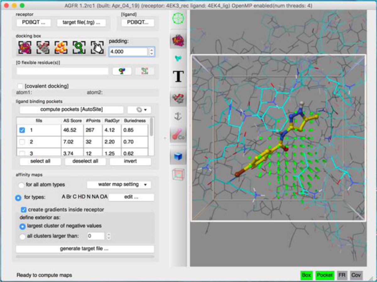
AFGR graphical User Interface.
The program was designed to facilitate common tasks in preparing a receptor for docking. While the docking box can be defined manually, it can also be positioned and sized based on a known ligand, or to cover a binding pocket identify by AutoSite, or outlined by a list of residues. It allows the specification of receptor side chains to be made flexible during the docking, or the specification of a covalent bond for docking covalently bound ligands. It supports both versions of the AutoSite pocket prediction algorithm and offers the option to add the affinity gradients discussed above to the maps. More details on these capabilities are provided in a series of online tutorials in the documentation section of the AGFR website22 covering various docking scenarios and the corresponding AGFR-based receptor preparation procedures.
The GUI is designed to guide users through the process, informing them of the next possible steps in the status bar located at the bottom of the interface. The button triggering the final calculation of the maps and the generation of the target file is only enabled once a basic set of requirements are fulfilled, e.g. the box needs to overlap with receptor and with a fill, all flexible receptor side chains need to be covered by the box, etc. The status of these requirements is indicated by the red/green light at the bottom right of the GUI.
In addition to specifying the docking box and computing the maps, AFGR supports the visual analysis of affinity maps using isocontours and/or orthographic slices of the maps, completed with a color map editor (Figure 4).
Figure 4:
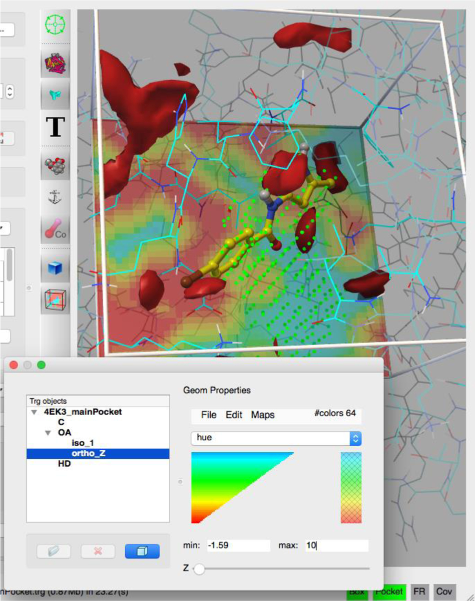
map visualization. A high-affinity isocontour of the oxygen maps is displayed along with an orthogonal slice of the Z plane.
When used from the command line, AGFR can perform an automatic analysis of a receptor to detect potential pocket and generate multiple target files for the top ranking binding sites. This feature greatly simplifies efficient blind docking experiments by performing multiple focused dockings potentially in parallel, rather than a single docking with a large box covering the entire receptor.
AGFR is written in the Python programming language23 and uses the Qt library24 for its GUI. It is available for the Linux, Max OS, and Windows operating systems. The software is available under the LGPL v2.0 license and can be downloaded from the AGFR website22.
Conclusion
We presented AutoGridFR (or AGFR), a new software program that facilitates the definition of docking boxes and the calculation of AutoDock4 affinity maps for them. It supports the preparation of receptors for advanced docking scenarios, including: docking covalently bound ligands, hydrated docking, and docking into receptors with flexible side chains. It also supports users in managing affinity maps by storing them in a single container file, together metadata that supports data provenance and promotes docking reproducibility. These target files are used as input by our newest docking engines AutoDockFR and AutoDock CrankPep. While the affinity maps are fully backwards compatible and can be extracted from a target file and used directly as input for AutoDock 4.2, we are planning to add support for them to the next release of AutoDock4. We also describe algorithms available in AGFR for improving affinity maps by adding gradients and improving binding site descriptors. Finally, a modern graphical user interface supports novice as well as expert users in preparing receptors for computational docking experiments.
Acknowledgments
The research reported in this publication was supported by the National Institute of General Medical Sciences of the National Institutes of Health under Award Number R01GM096888 to Dr. M. F. Sanner. The content is solely the responsibility of the authors and does not necessarily represent the official views of the National Institutes of Health. The authors also thank the members of the Center for Computational Structural Biology at Scripps Research La Jolla for many fruitful discussions. This is manuscript 29827 from The Scripps Research Institute.
References and Notes
- [1].Morris GM, Ruth H, Lindstrom W, Sanner MF, Belew RK, Goodsell DS, Olson AJ, J. Comput. Chem, 2009, DOI: 10.1002/jcc.21256. [DOI] [PMC free article] [PubMed] [Google Scholar]
- [2].Sousa SF, Ribeiro AJM, Coimbra JTS, Neves RPP, Martins SA, Moorthy NSHN, Fernandes PA, Ramos MJ, Curr. Med. Chem, 2013, 20. [DOI] [PubMed] [Google Scholar]
- [3].Trott O, Olson AJ, J. Comput. Chem, 2010, DOI: 10.1002/jcc.21334. [DOI] [PMC free article] [PubMed] [Google Scholar]
- [4].Forli S, Olson AJ, J. Med. Chem, 2012, DOI: 10.1021/jm2005145. [DOI] [PMC free article] [PubMed] [Google Scholar]
- [5].Johnson GT, Goodsell DS, Autin L, Forli S, Sanner MF, Olson AJ, Faraday Discuss, 2014, DOI: 10.1039/c4fd00017j. [DOI] [PMC free article] [PubMed] [Google Scholar]
- [6].Bianco G, Forli S, Goodsell DS, Olson AJ, Protein Sci, 2016, DOI: 10.1002/pro.2733. [DOI] [PMC free article] [PubMed] [Google Scholar]
- [7].Forli S, Botta M, J. Chem. Inf. Model, 2007, DOI: 10.1021/ci700036j. [DOI] [PubMed] [Google Scholar]
- [8].Harris R, Olson AJ, Goodsell DS, Proteins Struct. Funct. Bioinforma, 2008, DOI: 10.1002/prot.21645. [DOI] [Google Scholar]
- [9].Ravindranath PA, Sanner MF, Bioinformatics, 2016, DOI: 10.1093/bioinformatics/btw367. [DOI] [PMC free article] [PubMed] [Google Scholar]
- [10].Seeliger D, de Groot BL, J. Comput. Aided. Mol. Des, 2010, DOI: 10.1007/s10822-010-9352-6. [DOI] [PMC free article] [PubMed] [Google Scholar]
- [11].Cerqueira NMFSA, Ribeiro J, Fernandes PA, Ramos MJ, Int. J. Quantum Chem, 2011, DOI: 10.1002/qua.22738. [DOI] [Google Scholar]
- [12].Vaqué M, Arola A, Aliagas C, Pujadas G, Bioinformatics, 2006, DOI: 10.1093/bioinformatics/btl197. [DOI] [PubMed] [Google Scholar]
- [13].Dagum L, Menon R, Comput. Sci. Eng. IEEE, 1998, 5, 46–55. [Google Scholar]
- [14].Stoffler D, Coon SI, Huey R, Olson AJ, Sanner MF, in Proceedings of the 36th Annual Hawaii International Conference on System Sciences, HICSS 2003; 20032003. [Google Scholar]
- [15].Sanner MF, Olson AJ, Spehner J-C, in Proceedings of the Annual Symposium on Computational Geometry; 19951995.
- [16].Solis FJ, Wets RJ-B, Math. Oper. Res. - MOR, 1981, DOI: 10.1287/moor.6.1.19. [DOI] [Google Scholar]
- [17].Ravindranath PA, Forli S, Goodsell DS, Olson AJ, Sanner MF, PLoS Comput. Biol, 2015, DOI: 10.1371/journal.pcbi.1004586. [DOI] [PMC free article] [PubMed] [Google Scholar]
- [18].Zhang Y, Sanner M, Bioinformatics, 2019, DOI: 10.1093/bioinformatics/btz459. [DOI] [PMC free article] [PubMed] [Google Scholar]
- [19].Hartshorn MJ, Verdonk ML, Chessari G, Brewerton SC, Mooij WTM, Mortenson PN, Murray CW, J. Med. Chem, 2007, DOI: 10.1021/jm061277y. [DOI] [PubMed] [Google Scholar]
- [20].Hauser AS, Windshügel B, J. Chem. Inf. Model, 2016, DOI: 10.1021/acs.jcim.5b00234. [DOI] [PubMed] [Google Scholar]
- [21].Jaccard coefficent of similarity, https://www.statisticshowto.datasciencecentral.com/jaccard-index/.
- [22].Sanner MF, AGFR website, https://ccsb.scripps.edu/agfr.
- [23].van Rossum Guido, Python, http://www.python.org.
- [24].Qt 4.8, https://doc.qt.io/archives/qt-4.8/.