Distinguishing Felsenstein Zone from Farris Zone Using Neural Networks

Abstract

Maximum likelihood and maximum parsimony are two key methods for phylogenetic tree reconstruction. Under certain conditions, each of these two methods can perform more or less efficiently, resulting in unresolved or disputed phylogenies. We show that a neural network can distinguish between four-taxon alignments that were evolved under conditions susceptible to either long-branch attraction or long-branch repulsion. When likelihood and parsimony methods are discordant, the neural network can provide insight as to which tree reconstruction method is best suited to the alignment. When applied to the contentious case of Strepsiptera evolution, our method shows robust support for the current scientific view, that is, it places Strepsiptera with beetles, distant from flies.

Introduction

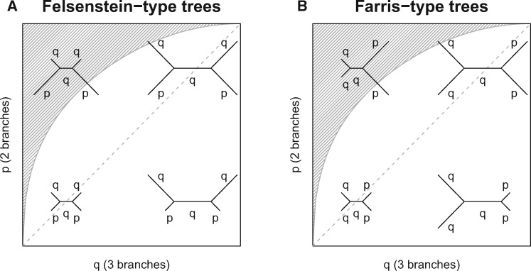
The phylogenetic artifact known as long-branch attraction (LBA) was first brought to attention in Felsenstein’s seminal paper (Felsenstein 1978), and subsequently elaborated on by Hendy and Penny (1989). They describe LBA succinctly, as the phenomena whereby “two long-branched, nonsister taxa are grouped together, rather than with their shorter branched sister taxa” when performing inference by maximum parsimony (MP). In recent years, LBA has, to some extent, lost its precise meaning (Sanderson et al. 2000; Bergsten 2005), but for the sake of clarity we will use the term LBA sensu stricto. The simplest form of LBA occurs in a four-taxon tree, with two long branches and three short branches as displayed in the upper left area of figure 1A. When the long branches are substantially larger than the short branches, MP is statistically inconsistent. That is, it will fail to reconstruct the true evolutionary history, instead grouping the taxa with the long branches in one clade, even with infinite sequence length. On the other hand, in the same scenario, maximum likelihood (ML) inference is statistically consistent. Given infinite sequence length, ML will recover the true tree, assuming the correct model of sequence evolution. Huelsenbeck and Hillis (1993) coined the term “Felsenstein zone” to refer to parameter combinations for which MP was inconsistent (see fig. 1).

Fig. 1.

Visualization of Felsenstein-type (A) and Farris-type tree topologies (B) for varying p and q, which describe the probabilities of observing a substitution at a particular site. The shaded area depicts the “Felsenstein zone.” At the dashed diagonal p equals q.

However, the asymptotic behavior of the reconstruction methods is of limited relevance, given the finite sequence lengths of biological data. In practice, the principal concerns relate to whether LBA is a relevant issue with biological data sets; and if so, the efficiency of tree reconstruction methods (Hillis et al. 1994) in the presence of LBA.

Although LBA was conclusively demonstrated using simulations by the late 1980s, considerable debate centered on whether this artifact was only of theoretical interest or could actually manifest in biological data sets. The first biological example of LBA was introduced by Carmean and Crespi (1995), arguing that the LBA artifact was responsible for the placement of Strepsiptera as sister to Diptera among insects. Their conclusion was challenged by Huelsenbeck (1997), who discussed the lack of evidence for LBA and suggested a simulation-based method to detect whether branches are long enough to be attracted by parsimony. He also pointed out the need for an unbiased reconstruction method that was not affected by LBA. Subsequently, Siddall (1998) asserted that LBA was not a significant issue in practice, showing that a similar effect in the opposite direction could also be demonstrated through simulation on four taxa. By constructing the true tree such that the long branches were in fact sisters, Siddall showed that parsimony was more efficient than likelihood in reconstructing the phylogeny (although likelihood methods remained consistent). He coined the parameter combinations for which parsimony was more efficient than likelihood, the “Farris zone.” Further, he reasoned that since the truth was unknowable in real data sets, when faced with discordance between parsimony and likelihood methods, it would be impossible to tell whether two long branches grouped together had been resolved correctly or not. This argument has held firm ever since.

The application of machine learning to evolutionary biology has primarily focused on the area of population genetics (Schrider and Kern 2018). The only machine learning contributions to phylogenetic tree reconstruction were recently made by Suvorov et al. (2020), who trained a network to infer four-taxon trees based on DNA sequences, whereas Zou et al. (2020) trained networks to do the same for amino acid alignments. Rather than attempting to design a single network that can infer tree topologies from empirical data sets generally, we opt for a different approach. We focus on resolving the topology of contentious data sets, specifically those for which MP and ML are discordant. To do so, we design and train neural networks specific to a single problem or empirical data set.

With our first network, F-zoneNN, we demonstrate that a simple, feedforward neural network can distinguish between alignments derived from a Felsenstein-type tree (two long branches in a four-taxon tree separated by a short internal edge; see fig. 1A) and a Farris-type tree (two long branches forming a cherry; fig. 1B). Feedback from the network can then be used to inform reconstruction method selection. With our second network, StrepsipteraNN, we show that, contrary to Sidall’s contention, a neural network can provide a robust conclusion as to the presence or absence of LBA in empirical data sets.

New Approaches

Neural Network

Neural networks are computing systems that attempt to emulate particular features of the biological brain of sentient beings, namely the ability to learn from experience. A neural network is trained by inputting large amounts of data with known output values. The network is then exposed to new data, which it classifies based on its training. Inspired by recent advances in the application of neural networks to a wide range of problems, in particular its strength in pattern recognition (Goodfellow et al. 2016 and references therein), we designed F-zoneNN, a feedforward neural network (e.g., Nielsen 2015), to classify multiple sequence alignments according to their generating tree types (i.e., whether they are Felsenstein-type or Farris-type). A detailed overview of F-zoneNN’s architecture can be found in table 2. To arrive at the architecture of F-zoneNN, we experimented with a range of different hyperparameters (Goodfellow et al. 2016), such as number and size of hidden layers.

Table 2.

Architecture and Hyperparameters of F-zoneNN for Simulated Alignments Using the Jukes–Cantor model and StrepsipteraNN Data Based on Strepsiptera Data of Carmean and Crespi (1995).

	F-ZoneNN	StrepsipteraNN
Number of nodes in layers	15, 64, 128, 256, 512, 1,024, 408, 208, 96, 1	256, 382, 512, 892, 1,024, 2,048, 808, 408, 324, 208, 96, 1
Transfer function (hidden layers)	ReLU	ReLU
Activation function (output layer)	Sigmoid	Sigmoid
Weight initialization	Xavier initialization (Glorot and Bengio 2010)	Xavier initialization (Glorot and Bengio 2010)
Bias initialization	Zero initialization	Zero initialization
Learning rate	0.0001	0.00001
Batch size	32	32
Cost function	Sigmoid cross-entropy	Sigmoid cross-entropy
Optimizer	Adam (Kingma and Ba 2015)	Adam (Kingma and Ba 2015)
Data set size per epoch	270,000,000 frequency vectors	552,960,000 frequency vectors
Epochs trained	2	3

Data Preprocessing

To encode multiple sequence alignments into a suitable format for F-zoneNN, we computed the site-pattern frequencies of each alignment. For four taxa, 256 unique site-patterns exist for the four-letter DNA alphabet. When using the JC model (Jukes and Cantor 1969), the 256 site-patterns collapse to 15 distinct pattern-categories, due to the symmetries in the substitution model. These are xxxx, xxxy, xxyx, xyxx, xxyy, xxyz, xyxy, xyyx, xyyy, xyxz, xyyz, xyzx, xyzy, xyzz, xyzw, where x, y, z, and w denote different nucleotides. For each branch length combination (p, q) the probabilities of the 15 patterns can be computed analytically (Felsenstein 2004, p. 111), thus generating a 15-dimensional multinomial distribution MD(p, q). The parameters p and q describe the probabilities of observing a substitution at a particular site along that branch (fig. 1).

Data Simulation

To keep everything simple and well defined, we assumed the JC model of sequence evolution for our initial experimental setup. Figure 1 shows the two trees that have a parameter p for two branches and a parameter q for three branches, for different (p, q) combinations.

We distinguish between Felsenstein/Farris zone and Felsenstein-/Farris-type trees. The Felsenstein zone is defined by the classical definition following Felsenstein (1978), the area of the parameter space where MP is statistically inconsistent, indicated by the shaded area in figure 1A. However, the Farris zone is not unambiguously defined for ML inference as its boundary depends on the length of the sequence alignment. To avoid this ambiguity, we simulate four-taxon trees for the full range of parameter (p, q) combinations. It should therefore be noted that the trees are indistinguishable if p = q and will switch from two long branches to three long branches when p is smaller than q (fig. 1).

We independently varied p and q over their entire range, from a minimum of 0.005 to a maximum of 0.745 at increments of 0.01. This created a total of 75×75 = 5,625 different parameter combinations. For each combination of p and q, 1,000 training alignments were generated. Each alignment was created by sampling 1,000 pattern-categories from the multinomial distribution MD(p, q). When carrying out the simulation-based training of F-zoneNN, we are aware which taxon belongs to which branch (i.e., which are from short branches and which are from the long branches). When analyzing test alignments, we do not have this luxury, and so F-zoneNN must be able to accurately classify alignments independent of the order of the taxa. To achieve this, we permuted the training data such that each simulated alignment was presented to F-zoneNN 24 times, once for each different ordering of the four taxa.

Test alignments were generated for a more sparsely populated grid of p and q combinations. The parameters varied between 0.025 and 0.725 at increments of 0.05, creating a total of 15×15 = 225 parameter combinations. For each combination of p and q, we used the program Seq-Gen (Rambaut and Grassly 1997) to simulate 200 different multiple sequence alignments of length 1,000 nucleotides. The training and test alignments were converted into vectors containing the relative pattern-category frequencies. The pattern-category frequencies served as input for F-zoneNN and the classical unweighted MP analysis, whereas the alignments served as input for phylogenetic inference using ML with IQ-TREE (Nguyen et al. 2015).

Analysis of Biological Data

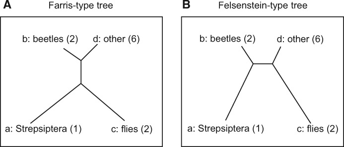
We revisited the well-known problem of placing Strepsiptera in the phylogenetic tree of insects (Carmean and Crespi 1995; Huelsenbeck 1997; Whiting et al. 1997). The historical discussion considered two different placements: one where Strepsiptera groups with flies and the other one where Strepsiptera groups with beetles. The two competing hypotheses are depicted in figure 2. The alignment comprises 18S ribosomal DNA sequences of 13 Holometabola insect species: (a) Strepsiptera (twisted-wing parasites: 1 sequence), (b) 2 Coleoptera (beetles: Tenebrio and Meloe), (c) 2 Diptera (flies: Aedes and Drosophila), and (d) 6 other Holometabola (Flea, Scorpionfly, Lacewing, Antlion, Sawfly, Polistes) and two outgroup Hemipteran sequences (Cercopidae and Cicada). Following Huelsenbeck (1997), we removed all sites with gaps and unknown DNA characters.

Fig. 2.

The two competing phylogenies discussed in Huelsenbeck (1997): Strepsiptera placed with (A) flies and (B) beetles relative to the other Holometabola. The number of sequences per group is indicated in parentheses.

We sampled groups of four taxa from the original 13-taxon alignment, such that each sampled quartet contained one taxon from each of the four groups (excluding the outgroup taxa). This resulted in 24 different quartets (1 Strepsiptera×2 beetles×2 flies×6 others). For each quartet, we constructed a Felsenstein-type (Strepsiptera grouped with beetles) and Farris-type (Strepsiptera grouped with flies) quartet tree. We then estimated the five branch lengths for all quartet trees using IQ-TREE, assuming the following substitution models: JC (Jukes and Cantor 1969), K2P (Kimura 1980), F81 (Felsenstein 1981), HKY (Hasegawa et al. 1985), TN (Tamura and Nei 1993), GTR (Tavaré 1986), and their respective Gamma-variants (+G; Yang 1994). Since α (the rate heterogeneity parameter of the Gamma distribution) is more reliably estimated from more taxa, we estimated α and the substitution model parameters from the original 13-taxon alignment. To control for the potential effect of the outgroups on the parameter estimates, we obtained a second estimate of these parameters from the 11-taxon alignment obtained by removing the two Hemipteran taxa. This resulted in 24×2×12×2 = 1,152 different tree/model/parameter combinations (24 quartets, 2 tree types, 12 substitution models, and 2 sets of α and substitution model parameter estimates based on the 13- and 11-taxon alignment).

Similarly to the F-zoneNN approach, we again experimented with a range of hyperparameters, and identified the best performing network. The architecture of the resulting network, StrepsipteraNN, is shown in table 2. StrepsipteraNN is a feedforward neural network, which takes 256 site-pattern frequencies as input.

For each unique tree/model/parameter combination, we used Seq-Gen to simulate 20,000 alignments of 1,000 bp. For each of these alignments, the order of taxa were permuted as before, resulting in a total of 1,152×20,000×24 = 552,960,000 training alignments.

In addition, we generated a test data set in order to assess the performance of StrepsipteraNN. Using Seq-Gen, we simulated 10 alignments of 1,000 bp for each of the above used 1,152 tree/model/parameter combinations. Again for each of those alignments the order of taxa was permuted, creating a total of 1,152×10×24 = 276,480 alignments.

Results and Discussion

Simulation Study

Inferring Tree Type

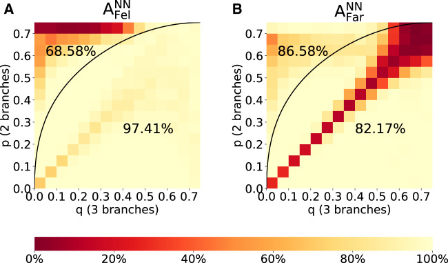
We define the notation${\mathrm{ }A}_{\mathrm{tree}\mathrm{ }\mathrm{type}}^{\mathrm{METHOD}}$ to refer to the accuracy of a given method for a particular tree type. Method will be one of MP, ML, NN, nogap300k (a network of Suvorov et al. [2020]), or Mix (abbreviation of Mixed strategy, to be defined later). Tree type will be either “Fel” or “Far” to indicate Felsenstein- or Farris-type trees, respectively. If no tree type is stipulated then the accuracy refers to all tree types. Figure 3 shows the accuracy of F-zoneNN to infer the correct Felsenstein-/Farris-type tree. For the largest fraction of the parameter space, F-zoneNN was able to distinguish whether an alignment originated from Felsenstein-type or Farris-type trees. Felsenstein-type alignments were successfully identified to a high degree of accuracy (97.41%) outside of the Felsenstein zone. The few misclassifications occurred primarily on the diagonal, where the two tree types are not distinguishable. Within the Felsenstein zone, F-zoneNN identified Felsenstein-type trees with 68.58% accuracy. However, the majority of misclassifications occur at biologically unrealistically high values of p. Farris-type alignments are successfully classified over the entire parameter space, except along the main diagonal, and when both p and q are unrealistically high.

Fig. 3.

Accuracy of F-zoneNN to infer the correct tree type under a Felsenstein-type tree (A) and Farris-type tree (B) for sequence alignments of length 1,000 bp. In each plot, the region above the curve reflects the Felsenstein zone, and the region below reflects the (p, q)-combinations where MP is consistent. Accordingly, the percentage above the curve denotes the accuracy of F-zoneNN in the Felsenstein zone and the number below the accuracy outside the Felsenstein zone. For detailed accuracy values see supplementary figure S1, SupplementaryMaterial online.

F-zoneNN cannot distinguish the data if p = q as the trees are identical (cf. the diagonal in fig. 3B), but we notice that in this region it tends to label these trees as Felsenstein-type. This is of no real consequence, as the two tree types are identical in this circumstance, and therefore no classification can reasonably be considered correct or incorrect.

Inferring Tree Topology

Given a sequence alignment, F-zoneNN does not output a tree topology, it simply classifies the alignment as being either Felsenstein- or Farris-type. In order to reconstruct the topology for a given alignment, we must rely on one of the traditional methods, MP or ML. The decision to use MP or ML is entirely dependent on the output of F-zoneNN. For a given test alignment, if F-zoneNN classifies it as a Felsenstein-type tree, then the Mixed strategy will return the tree inferred by ML. This follows from the fact that, in the absence of prior information about p and q, we know that ML is more likely to infer the correct topology than MP, for a Felsenstein-type tree. Similarly, if F-zoneNN indicates a Farris-type tree then the Mixed strategy will return the tree inferred by MP, as for Farris-type trees MP is more likely to infer the correct topology than ML. It must be made explicit that the accuracies reported in figure 3 refer only to the success of F-zoneNN in inferring the correct tree type. They do not represent the accuracy of F-zoneNN inferring the correct topology. To avoid confusion, we refer to the process of topological inference using F-zoneNN to inform reconstruction method selection as the “Mixed” strategy.

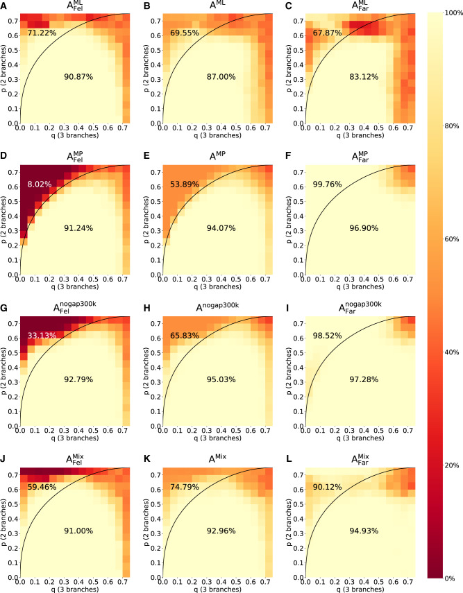
Figure 4 shows the accuracy of ML (first row) and MP (second row) assuming a Felsenstein-type tree (first column), a Farris-type tree (third column), and the average accuracy (middle column) independent of the tree type. The third row of figure 4 shows the accuracies for nogap300k, a convolutional neural network that reconstructs four-taxon trees based on a multiple sequence alignment. nogap300k was the best performing network for our test data among the networks trained by Suvorov et al. (2020). The fourth row of figure 4 shows the results for the Mixed strategy. A summary of the accuracy of the four methods across the tree types and within the Felsenstein zone is provided in table 1.

Fig. 4.

Accuracies of phylogenetic reconstruction using ML (A–C), MP (D–F), and nogap300k (Suvorov et al. 2020) (G–I), as well as the accuracy to reconstruct the tree using the Mixed strategy involving F-zoneNN, MP, and ML (J–L). In each plot, the region above the curve reflects the Felsenstein zone and the region below reflects the (p, q)-combinations, where MP is consistent. Accordingly, the percentage above the curve denotes the accuracy of the respective method in the Felsenstein zone, and the percentage below the curve denotes the accuracy outside the Felsenstein zone. For detailed accuracy values see supplementary figures S2–S5, SupplementaryMaterial online.

Table 1.

Accuracies of Phylogenetic Reconstruction Using ML, MP, nogap300k and the Mixed Strategy over All Felsenstein-Type Trees and All Farris-Type Trees of the Test Data Set As Well As the Average Accuracies Computed from the Second and Third Table Column.

Method	Felsenstein Zone	Outside Felsenstein Zone	Felsenstein-Type Trees	Farris-Type Trees	Average Accuracy
Maximum likelihood	69.55%	87.00%	87.03%	80.14%	83.58%
Maximum parsimony	53.89%	94.07%	74.97%	97.46%	86.21%
nogap300k	65.83%	95.03%	81.12%	97.52%	89.32%
Mixed strategy	74.79%	92.96%	84.84%	93.99%	89.41%

The accuracies of ML and MP as depicted in figure 4A, C, D, and F reflect the well-known behavior of these reconstruction methods. Suvorov et al. appear to have trained a network that closely mimics (although improves upon) the performance of MP (fig. 4F and I). Consequently, their network performs poorly (33%) in the Felsenstein zone, as opposed to ML (71%). The Mixed strategy is indeed a mix between MP and ML. Although it is closer to MP for Farris-type trees, it performs better (and closer to ML) for Felsenstein-type trees. F-zoneNN’s output has no practical consequences for the Mixed strategy for the indistinguishable trees where p = q, since MP and ML both perform well in this area. Among all reconstruction methods, the average accuracy of the Mixed strategy is highest, albeit only marginally better than nogap300k. The Mixed strategy outperforms nogap300k for Felsenstein-type trees, but is outperformed by nogap300k for Farris-type trees. In the Felsenstein zone, which is of specific interest for our task, the Mixed strategy outperformed nogap300k as well as the standard approaches (fig. 4, middle column). Therefore, the Mixed strategy is more suitable for the problem of distinguishing Farris-type and Felsenstein-type trees.

Resolving Disputed Topologies

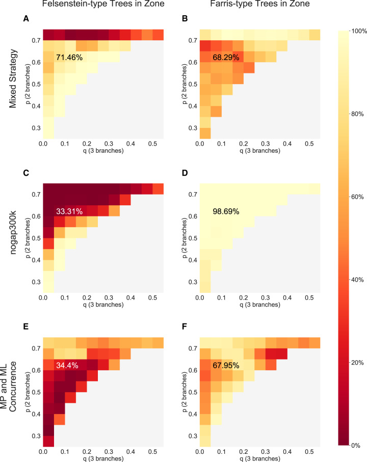
Recalling that the primary goal of the research is to resolve disputed topologies, it makes sense to pay particular attention to alignments for which MP and ML infer conflicting tree topologies. We therefore restricted our interest to alignments whereby, owing to their presence in either the Felsenstein or Farris zone, MP and ML return conflicting topologies. Further, it is elementary to realize that in cases where MP and ML agree, then the output of F-zoneNN is not relevant to the performance of the Mixed strategy. Figure 5 shows the results of the Mixed strategy and nogap300k within the Felsenstein/Farris zone, for alignments in which MP and ML reconstruct different topologies. The tendency for the nogap300k network to emulate MP is stark here. For contentious Farris-type trees, nogap300k infers the correct tree almost 99% of the time. Its performance for contentious Felsenstein-type trees is much less reliable, only inferring the correct topology ∼33% of the time. This illustrates the susceptibility of nogap300k to the LBA artifact, much like MP.

Fig. 5.

Summary of accuracies within the Felsenstein zone, on simulated test alignments for which MP and ML inferred conflicting trees. Accuracies of phylogenetic reconstruction are compared using the Mixed strategy (A and B) and nogap300k (Suvorov et al. 2020) (C and D). The proportion of test alignments for which MP and ML agree is also shown (E and F). Felsenstein-type alignments are shown in the first column, whereas Farris-type alignments are shown in the second column.

Conversely, the Mixed strategy provides more balanced results. Whether the true tree is Felsenstein- or Farris-type, the Mixed strategy reconstructs the correct topology at similar rates (71.46% and 68.29%, respectively). Furthermore, the heatmap in figure 5A shows that the accuracy of the Mixed strategy is excellent in all areas of the Felsenstein zone, except for very high values of p. It might be argued that the clear superior performance of the Mixed strategy over nogap300k for Felsenstein-type trees, is offset by its inferior performance for Farris-type trees. However, we would argue that when considering empirical data sets Felsenstein-type trees are much more likely to be observed. This follows from the simple logic that, given two long branches, there are many more ways for them to be placed apart on a tree (Felsenstein-type), than together (Farris-type). Additionally, figure 5E and F illustrates that there is significant disparity between tree types, in the proportion of alignments that are contentious. For Felsenstein-type trees in the Felsenstein zone, only 34.4% resulted in concurrence between MP and ML. The methods concurred for nearly twice as many, 67.95%, of Farris-type trees. Furthermore, the p, q combinations where MP and ML are least likely to concur (dark red in fig. 5E) correspond to areas within the Felsenstein zone for which the Mixed strategy performs very well (light areas of fig. 5A).

The Impact of Alignment Length

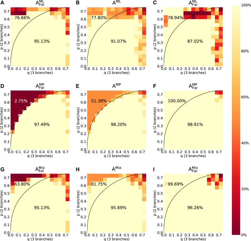
To assess the impact of the alignment length, $l$, we computed $A^{\mathrm{Mix}}$ for alignments of various lengths up to 10,000 bp. With increasing sequence length, the accuracy of F-zoneNN improves (see fig. 6). More precisely for alignments of length 10,000 bp $A^{\mathrm{Mix}}$ is 92.98%, whereas $A^{\mathrm{ML}}$ is only 88.48% and $A^{\mathrm{MP}}$ is 89.04%. The networks of Suvorov et al. cannot process alignments of length 10,000 bp because the input alignments of the convolutional neural networks used by Suvorov et al. (2020) are fixed to specific lengths. Conversely, F-zoneNN has the flexibility to accept alignments of any length.

Fig. 6.

Accuracies of phylogenetic reconstruction using ML (A–C) and MP (D–F) as well as the accuracy to reconstruct the tree using the Mixed strategy involving F-zoneNN, MP, and ML (G–I) on alignments of length 10,000 bp. In each plot, the region above the curve reflects the Felsenstein zone, and the region below reflects the (p, q)-combinations where MP is consistent. Accordingly, the percentage above the curve denotes the accuracy of the respective method in the Felsenstein zone, and the percentage below the curve denotes the accuracy outside the Felsenstein zone.

Analysis of Biological Data

We tested the StrepsipteraNN on the simulated test data. We then used StrepsipteraNN to classify the 576 empirical quartet alignments (24 distinct alignments, each with the order of taxa permuted in all 24 possible ways).

The StrepsipteraNN was able to successfully distinguish between Felsenstein-type and Farris-type trees on the simulated test data. It correctly classified 87.30% of the Felsenstein-type trees and 90.91% of the Farris-type trees (89.11% of all trees).

Of the 24×24 = 576 empirical quartet alignments (24 quartets and 24 permutations of each), StrepsipteraNN infers a Felsenstein-type tree 574 times. Only for two permutations of a specific quartet did StrepsipteraNN infer a Farris-type tree. Therefore, it supports the placement of Strepsiptera as sister to beetles (cf. fig. 2B), as opposed to flies. In light of the high level of accuracy achieved on classifying test data, the concurrent classification of 99.7% of the empirical alignments is compelling. Furthermore, the grouping of Strepsiptera with beetles is in concordance with the conclusions of the most recent literature on the topic (Niehuis et al. 2012; Boussau et al. 2014).

We demonstrate here that it is possible, through the application of machine learning technology to phylogenetic questions, to challenge Siddall’s (1998) reasoning that the truth was unknowable when MP and ML conflict. Although we cannot claim to “know” with certainty the true placement of Strepsiptera, we can train a neural network to find patterns in the data that offer strong support to one hypothesis over the other.

We expect that the method we demonstrate here can be easily adapted to other empirical data sets in which MP and ML prove inconclusive. However, we see no reason that our approach would be limited to the presence/absence of LBA. The increasing prevalence of phylogenomic data sets, in which alignments consist of many genes/loci, has led to the development of increasingly complex models of sequence evolution. The presence of heterotachy as described by Lopez et al. (2002) (sites that evolve at different rates on different lineages) is all but assured in such data sets, because genes are subject to different functional constraints in different species. As such, models of sequence evolution that can account for heterotachy, for example, partition models (Lanfear et al. 2017) or mixture models such as GHOST (Crotty et al. 2020), are recommended for phylogenomic analyses. However, such analyses can result in discordance among topologies inferred under different models/methods. We see no reason that the method outlined here could not be easily adapted to such situations. One could train a network using data simulated from the parameters inferred under each of the competing models/methods, validate that the network can accurately classify testing data simulated under the same models, and then feed the network all informative quartets (those that induce different quartet trees under the two competing models) from the empirical data and see if a conclusive result is returned.

Conclusion

We have explored a well-known Achilles heel of phylogenetic inference, LBA, and demonstrated that neural networks can be employed to inform the choice of phylogenetic inference method, potentially improving accuracy and increasing efficiency. Moreover, our results show that our relatively simple neural network outperforms the complex convolutional neural network. Further, we show that the application of our method to a data set that has been contentious in the literature, with some considering it an example of LBA and others not, yields results consistent with the currently accepted phylogeny. This initial study illustrates the potential of neural networks to be applied to the tree inference problem. Our approach suggests that in the face of topological discordance among competing inference methods, machine learning techniques may be able to point toward the underlying biological truth.

In this study, we have only scratched the surface of the potential of deep learning approaches to be utilized in the field of phylogenetic inference. We also note that our and Suvorov’s et al. (2020) applications, although in spirit similar, show distinguished differences. Our approach accepts alignments of any length but strictly without gaps, whereas the approach of Suvorov et al. (2020) requires a fixed alignment length but can accept gaps. More work is needed for understanding neural networks and their applications or limitations in this field. Certainly, a single neural network that can be used generally on a wide variety of empirical data is a lofty ambition. However, we have shown here that specialized neural networks can be designed and trained to address specific phylogenetic questions. Given there is no shortage of open problems in the field, phylogenetic inference seems to be fertile ground for the application of machine learning techniques.

Materials and Methods

Neural Network Architectures

F-ZoneNN and StrepsipteraNN as well as the used training and test data can be found at GitHub (https://github.com/Cibiv/zone-net). An overview of the networks’ architectures and hyperparameters is presented in table 2.

Supplementary Material

Supplementary data are available at Molecular Biology and Evolution online.

References

- Bergsten J. 2005. A review of long-branch attraction. Cladistics 21(2):163–193. [DOI] [PubMed] [Google Scholar]
- Boussau B, Walton Z, Delgado JA, Collantes F, Beani L, Stewart IJ, Cameron SA, Whitfield JB, Johnston JS, Holland PWH, et al. 2014. Strepsiptera, phylogenomics and the long branch attraction problem. PLoS One 9(10):e107709. [DOI] [PMC free article] [PubMed] [Google Scholar]
- Carmean D, Crespi BJ.. 1995. Do long branches attract flies. Nature 373(6516):666–666. [DOI] [PubMed] [Google Scholar]
- Crotty SM, Minh BQ, Bean NG, Holland BR, Tuke J, Jermiin LS, von Haeseler A.. 2020. GHOST: recovering historical signal from heterotachously evolved sequence alignments. Syst Biol. 69(2):249–264. [DOI] [PubMed] [Google Scholar]
- Felsenstein J. 1978. Cases in which parsimony or compatibility methods will be positively misleading. Syst Zool. 27(4):401–410. [Google Scholar]
- Felsenstein J. 1981. Evolutionary trees from DNA sequences: a maximum likelihood approach. J Mol Evol. 17(6):368–376. [DOI] [PubMed] [Google Scholar]
- Felsenstein J. 2004. Inferring phylogenies. Sunderland (MA: ): Sinauer. [Google Scholar]
- Glorot X, Bengio Y.. 2010. Understanding the difficulty of training deep feedforward neural networks In: Teh YW, Titterington M, editors. Proceedings of the Thirteenth International Conference on Artificial Intelligence and Statistics. Sardinia (Italy: ): PMLR; p. 249–256. [Google Scholar]
- Goodfellow I, Bengio Y, Courville A.. 2016. Deep learning. Cambridge (MA: ): MIT Press; Available from: http://www.deeplearningbook.org. [Google Scholar]
- Hasegawa M, Kishino H, Yano T.. 1985. Dating the human-ape splitting by a molecular clock of mitochondrial DNA. J Mol Evol. 22(2):160–174. [DOI] [PubMed] [Google Scholar]
- Hendy MD, Penny D.. 1989. A framework for the quantitative study of evolutionary trees. Syst Zool. 38(4):297–309. [Google Scholar]
- Hillis DM, Huelsenbeck JP, Swofford DL.. 1994. Hobgoblin of phylogenetics? Nature 369(6479):363–364. [DOI] [PubMed] [Google Scholar]
- Huelsenbeck JP. 1997. Is the Felsenstein zone a fly trap? Syst Biol. 46(1):69–74. [DOI] [PubMed] [Google Scholar]
- Huelsenbeck JP, Hillis DM.. 1993. Success of phylogenetic methods in the four-taxon case. Syst Biol. 42(3):247–264. [Google Scholar]
- Jukes TH, Cantor C.. 1969. Evolution of protein molecules In: Munro HN, editor. Mammalian protein metabolism. New York: Academic Press; p. 21–132. [Google Scholar]
- Kimura M. 1980. A simple method for estimating evolutionary rate of base substitutions through comparative studies of nucleotide sequences. J Mol Evol. 16(2):111–120. [DOI] [PubMed] [Google Scholar]
- Kingma D, Ba J.. 2015. Adam: a method for stochastic optimization Proceedings of the 3rd International Conference on Learning Representations (ICLR 2015). Ithaca (NY: ): arXiv.org; Available from: http://arxiv.org/abs/1412.6980. [Google Scholar]
- Lanfear R, Frandsen PB, Wright AM, Senfeld T, Calcott B.. 2017. PartitionFinder 2: new methods for selecting partitioned models of evolution for molecular and morphological phylogenetic analyses. Mol Biol Evol. 34(3):772–773. [DOI] [PubMed] [Google Scholar]
- Lopez P, Casane D, Philippe H.. 2002. Heterotachy, an important process of protein evolution. Mol Biol Evol. 19(1):1–7. [DOI] [PubMed] [Google Scholar]
- Nguyen L-T, Schmidt HA, von Haeseler A, Minh BQ.. 2015. IQ-TREE: a fast and effective stochastic algorithm for estimating maximum likelihood phylogenies. Mol Biol Evol. 32(1):268–274. [DOI] [PMC free article] [PubMed] [Google Scholar]
- Niehuis O, Hartig G, Grath S, Pohl H, Lehmann J, Tafer H, Donath A, Krauss V, Eisenhardt C, Hertel J, et al. 2012. Genomic and morphological evidence converge to resolve the enigma of Strepsiptera. Curr Biol. 22(14):1309–1313. [DOI] [PubMed] [Google Scholar]
- Nielsen MA. 2015. Neural networks and deep learning. San Francisco: Determination Press. Available from: http://neuralnetworksanddeeplearning.com/. [Google Scholar]
- Rambaut A, Grass NC.. 1997. Seq-Gen: an application for the Monte Carlo simulation of DNA sequence evolution along phylogenetic trees. Comput Appl Biosci. 13(3):235–238. [DOI] [PubMed] [Google Scholar]
- Sanderson MJ, Wojciechowski MF, Hu JM, Khan TS, Brady SG.. 2000. Error, bias, and long-branch attraction in data for two chloroplast photosystem genes in seed plants. Mol Biol Evol. 17(5):782–797. [DOI] [PubMed] [Google Scholar]
- Schrider DR, Kern AD.. 2018. Supervised machine learning for population genetics: a new paradigm. Trends Genet. 34(4):301–312. [DOI] [PMC free article] [PubMed] [Google Scholar]
- Siddall ME. 1998. Success of parsimony in the four‐taxon case: long‐branch repulsion by likelihood in the Farris zone. Cladistics 14(3):209–220. [DOI] [PubMed] [Google Scholar]
- Suvorov A, Hochuli J, Schrider D.. 2020. Accurate inference of tree topologies from multiple sequence alignments using deep learning. Syst Biol. 69(2):221–233. [DOI] [PMC free article] [PubMed] [Google Scholar]
- Tamura K, Nei M.. 1993. Estimation of the number of nucleotide substitutions in the control region of mitochondrial DNA in humans and chimpanzees. Mol Biol Evol. 10:512–526. [DOI] [PubMed] [Google Scholar]
- Tavaré S. 1986. Some probabilistic and statistical problems in the analysis of DNA sequences In: Miura RM, editor. Some mathematical questions in biology – DNA sequence analysis. Providence (RI: ): American Mathematical Society; p. 57–86. [Google Scholar]
- Whiting MF, Carpenter JC, Wheeler QD, Wheeler WC.. 1997. The Strepsiptera problem: phylogeny of the holometabolous insect orders inferred from 18S and 28S ribosomal DNA sequences and morphology. Syst Biol. 46(1):1–68. [DOI] [PubMed] [Google Scholar]
- Yang Z. 1994. Maximum likelihood phylogenetic estimation from DNA sequences with variable rates over sites: approximate methods. J Mol Evol. 39(3):306–314. [DOI] [PubMed] [Google Scholar]
- Zou Z, Zhang H, Guan Y, Zhang J.. 2020. Deep residual neural networks resolve quartet molecular phylogenies. Mol Biol Evol. 37(5):1495–1507. [DOI] [PMC free article] [PubMed] [Google Scholar]
Associated Data
This section collects any data citations, data availability statements, or supplementary materials included in this article.