Semiparametric Estimation with Data Missing Not at Random Using an Instrumental Variable

Abstract

Missing data occur frequently in empirical studies in health and social sciences, often compromising our ability to make accurate inferences. An outcome is said to be missing not at random (MNAR) if, conditional on the observed variables, the missing data mechanism still depends on the unobserved outcome. In such settings, identification is generally not possible without imposing additional assumptions. Identification is sometimes possible, however, if an instrumental variable (IV) is observed for all subjects which satisfies the exclusion restriction that the IV affects the missingness process without directly influencing the outcome. In this paper, we provide necessary and sufficient conditions for nonparametric identification of the full data distribution under MNAR with the aid of an IV. In addition, we give sufficient identification conditions that are more straightforward to verify in practice. For inference, we focus on estimation of a population outcome mean, for which we develop a suite of semiparametric estimators that extend methods previously developed for data missing at random. Specifically, we propose inverse probability weighted estimation, outcome regression-based estimation and doubly robust estimation of the mean of an outcome subject to MNAR. For illustration, the methods are used to account for selection bias induced by HIV testing refusal in the evaluation of HIV seroprevalence in Mochudi, Botswana, using interviewer characteristics such as gender, age and years of experience as IVs.

1. Introduction

Selection bias is a major problem in health and social sciences, and is said to be present in an empirical study if features of the underlying population of primary interest are entangled with features of the selection process not of scientific interest. Selection bias can occur in practice due to incomplete data, if the observed sample is not representative of the true underlying population. While various ad hoc methods exist to adjust for missing data, such methods may be subject to bias unless under fairly strong assumptions. For example, complete-case analysis is easy to implement and is routinely used in practice. However, complete-case analysis is well-known to generally produce biased estimates when the outcome is not missing completely at random (MCAR) (Little and Rubin, 2002). Progress can still be made if data are missing at random (MAR), such that the missing data mechanism is independent of unobserved variables conditional on observed data. Principled methods for handling MAR data abound, including likelihood-based procedures (Little and Rubin, 2002; Horton and Laird, 1998), multiple imputation (Rubin, 1987; Kenward and Carpenter, 2007a; Horton and Lipsitz, 2001; Schafer, 1999), inverse probability weighting (Robins et al., 1994; Tsiatis, 2007; Li et al., 2013) and doubly robust estimation (Scharfstein et al., 1999; Lipsitz et al., 1999; Robins et al., 2000; Robins and Rotnitzky, 2001; Neugebauer and van der Laan, 2005; Tsiatis, 2007; Tchetgen Tchetgen, 2009).

The MAR assumption is strictly not testable in a nonparametric model without an additional assumption (Gill et al., 1997; Potthoff et al., 2006) and is often untenable. An outcome is said to be missing not at random (MNAR) if it is neither MCAR nor MAR, such that conditional on the observed data, the missingness process remains dependent on the unobserved outcome (Little and Rubin, 2002). Identification is generally not available under MNAR without an additional assumption (Robins and Ritov, 1997). A possible approach is to make sufficient parametric assumptions (Little and Rubin, 2002; Roy, 2003; Wu and Carroll, 1988) about the full data distribution for identification. However, this approach can fail even with commonly used fully parametric models (Miao et al., 2014; Wang et al., 2014). Other existing strategies for MNAR include positing sufficiently stringent modeling restrictions on a model for the missing data process (Rotnitzky and Robins, 1997) or obtaining sensitivity analysis and bounds (Moreno-Betancur and Chavance, 2013; Kenward and Carpenter, 2007b; Robins et al., 2000; Vansteelandt et al., 2007). Another common identification approach involves leveraging an instrumental variable (IV) (Manski, 1985; Winship and Mare, 1992). Heckman’s framework (Heckman, 1979, 1997) is perhaps the most common IV approach used primarily in economics and other social sciences to account for outcome MNAR. A valid IV is known to satisfy the following conditions:

1. the IV is not directly related to the outcome in the underlying population, conditional on a set of fully observed covariates, and

2. the IV is associated with the missingness mechanism conditional on the fully observed covariates.

Therefore a valid IV must predict a person’s propensity to have an observed outcome, without directly influencing the outcome.

In principle, one can use a valid IV to obtain a nonparametric test of the MAR assumption. However access to an IV does not generally point identify the joint distribution of the full data nor its functionals. Heckman’s selection model (Heckman, 1979) is generally not identifiable without an assumption of bivariate normal latent error in defining the model (Wooldridge, 2010). Estimation using Heckman-type selection models may be sensitive to these parametric assumptions (Winship and Mare, 1992; Puhani, 2000), although there has been significant work towards relaxing some of the assumptions (Manski, 1985; Newey et al., 1990; Das et al., 2003; Newey, 2009). An alternative sufficient identification condition was considered by Tchetgen Tchetgen and Wirth (2013) which involves restricting the functional form of the selection bias function due to non-response on a given scale for the outcome (mean additive, mean multiplicative or logistic). However, as shown in simulation studies below, their approach is sensitive to bias due to model misspecification, and a more robust approach is warranted.

In this paper, we develop a general framework for nonparametric identification of selection models based on an IV. We describe necessary and sufficient conditions for identifiability of the full data distribution with a valid IV. For inference we focus on estimation of an outcome mean, although the proposed methods are easy to adapt to other functionals. We develop three semiparametric approaches that extend analogous methods previously developed for missing at random (MAR) settings: inverse probability weighting (IPW), outcome regression (OR) and doubly robust (DR) estimation. The consistency of each estimator relies on correctly specified models for parts of the full data law. Extensive simulation studies are used to investigate the finite sample properties of proposed estimators. For illustration, the methods are used to account for selection bias induced by HIV testing refusal in the evaluation of HIV seroprevalence in Mochudi, Botswana, using interviewer characteristics including gender, age and years of experience as IVs. All proofs are relegated to a Supplemental Appendix.

2. Notation and Assumptions

Suppose that one has observed n independent and identically distributed observations (X,RY,R,Z) with fully observed covariates X and R is the indicator of whether the person’s outcome Y is observed. The variable Z is a fully observed IV that satisfies assumptions (i) and (ii) formalized below. In the evaluation of HIV prevalence in Mochudi, X includes all demographic and behavioral variables collected for all persons in the sample, while HIV status Y may be missing for individuals who failed to be tested, i.e. with R = 0. Let $\tilde{\pi }(X,Z)=\text{Pr}(R=1\mid X,Z)$ denote the propensity score for the missingness mechanism given (X,Z). As a valid IV, we will assume that Z satisfies the following assumptions.

(IV.1) Exclusion restriction:

$$P_{Y\mid X,Z}(y\mid x,z)=P_{Y\mid X}(y\mid x)\text{ for all }x,z.$$

(IV.2) IV relevance:

$$\tilde{\pi }(x,z)-\tilde{\pi }\left(x,z^{\prime }\right)\ne 0\text{ for all }x.$$

Exclusion restriction (IV.1) states that the IV and the outcome are conditionally independent given X in the underlying population, that is the IV does not have a direct effect on the outcome, which places restrictions on the full data law. IV relevance requires that the IV remains associated with the missingness mechanism even after conditioning on X, which allows for full rank conditions in estimation. In spite of (IV.2), (IV.1) implies that Z cannot reduce the dependence between R and Y, therefore under MNAR π(x, y, z) = P(R = 1|x, y, z) remains a function of y even after conditioning on (x, z). In addition, (IV.1) and (IV.2) imply that under MNAR the IV remains relevant in π(x, y, z) conditional on (x, y). Both of these facts will be used repeatedly throughout. $\tilde{\pi }(x,z)$ is typically referred to as the propensity score for the missingness process, and we shall likewise refer to π(x, y, z) as the extended propensity score.

3. Identification

Although (IV.1) reduces the number of unknown parameters in the full data law, identification is still only available for a subset of all possible full data laws. As an illustration, consider the case of binary outcome and IV. For simplicity and without loss of generality, we omit covariates X. Assumption (IV.1) implies P(z, y) = P(y)P(z). We are only able to identify the quantities P(z, y|R = 1), P(z|R = 0), P(R = 1) from the observed data. These quantities are functions of the unknown parameters: P(Z = 1), P(Y = 1), and P(R = 1|z, y). So we have six unknown parameters, but only five available independent equations, one for each empirically identified parameter given above. As a result, the full data law is not identifiable, and P(Y = 1) is not identifiable.

The IV model becomes identifiable once one sufficiently restricts the class of models for the joint distribution of (Z, Y,R). Let ${\mathcal{P}}_{\theta }(R,Z,Y)$, ${\mathcal{P}}_{\eta }(Z)$ and ${\mathcal{P}}_{\xi }(Y)$ denote the collection of such candidates for P(R = 1|z, y), P(z) and P(y), respectively. Members of the sets are indexed by parameters θ, η and ξ, which may be infinite dimensional. The identifiability of the model is determined by the relationship between its members.

Theorem 1. Suppose that Assumption 1 holds, then the joint distribution P(z, y, r) is identifiable if and only if ${\mathcal{P}}_{\theta }(R,Z,Y)$ and ${\mathcal{P}}_{\xi }(Y)$ satisfy the following condition: for any pair of candidates

$$\left\{P_{{\theta }_1}(R=1\mid z,y),P_{{\xi }_1}(y)\right\}and\left\{P_{{\theta }_2}(R=1\mid z,y),P_{{\xi }_2}(y)\right\}$$

in the model the following inequality holds:

$$\frac{P_{{\theta }_1}(R=1\mid z,y)}{P_{{\theta }_2}(R=1\mid z,y)}\ne \frac{P_{{\xi }_2}(y)}{P_{{\xi }_1}(y)}$$ (3.1)

for at least one value of z and y.

Theorem 1 presents a necessary and sufficient condition for identifiability of the joint distribution of the full data, and thus a sufficient condition for identifiability of its functionals. We have the following corollary which provides a more convenient condition to verify.

Corollary 1. Suppose that Assumption 1 holds, then the joint distribution P(z, y, r) is identifiable if the ratio $P_{{\theta }_1}(R=1\mid z,y)/P_{{\theta }_2}(R=1\mid z,y)$ is either a constant or varies with z for any two elements $P_{{\theta }_1}(R,Z,Y)$ and $P_{{\theta }_2}(R,Z,Y)$ of the model.

Although Corollary 1 provides a sufficient condition for identification of the joint distribution of the full data, it is still possible to characterize the identifiability of a large class of parametric or semi-parametric models by verifying the condition in the corollary, which we illustrate with several examples.

Example 1. For binary outcome with binary instrument, consider the candidate set

$${\mathcal{P}}_{\theta }(R,Z,Y)=\left\{P(R=1\mid Z,Y)=\text{expit }\left[{\theta }_0+{\theta }_{1}Z+{\theta }_{2}Y+{\theta }_{3}ZY\right]:\left({\theta }_0,{\theta }_1,{\theta }_2,{\theta }_3\right)\in {ℝ}^4\right\},$$

which are saturated in (Z, Y). It is shown in the Supplemental Appendix that candidates from this set do not satisfy inequality (1) in Theorem 1 and therefore the joint distribution of (Z,Y,R) cannot be identified without reducing the dimension of ✓ through modeling assumptions. By Corollary 1, the joint distribution can be identified for the candidate set

$${\mathcal{P}}_{\theta }(R,Z,Y)=\left\{P(R=1\mid Z,Y)=\text{expit }\left[{\theta }_0+{\theta }_{1}Z+{\theta }_{2}Y\right]:\left({\theta }_0,{\theta }_1,{\theta }_2\right)\in {ℝ}^3\right\},$$

i.e. with the additional assumption that the association of the outcome Y with the missingness mechanism is constant within levels of Z, on the logit scale. A more general result on the identifiability of separable logistic missing data mechanisms, which also holds for continuous Y and Z, is given in Example 2.

Example 2. The separable logistic missing data mechanism

$${\mathcal{P}}_{\theta }(R,Z,Y)=\left\{P(R=1\mid Z,Y)=\text{expit}[q(Z)+h(Y)]\right\},$$ (3.2)

is identifiable, where q(·) and h(·) are unknown functions differentiable with respect to Z and Y respectively. Identification also holds if either Z or Y is binary or discrete random variables.

Example 3. The separable probit missing data data mechanism

$${\mathcal{P}}_{\theta }(R,Z,Y)=\left\{P(R=1\mid Z,Y)=\Phi [q(Z)+h(Y)]\right\},$$ (3.3)

is identifiable, where q(·) and h(·) are unknown functions assumed to be differentiable with respect to Z and Y respectively.

Example 4. Under MAR, the missing data mechanism

$${\mathcal{P}}_{\theta }(R,Z,Y)=\left\{P(R=1\mid Z,Y)=g(Z)\right\}$$ (3.4)

satisfies Corollary 1 and is identifiable. It is clear that the ratio of any pair of members is either a constant or varies with Z.

4. Estimation and Inference

In this section, we consider estimation and inference under a variety of semiparametric IV models known to satisfy Theorem 1. We denote the collection of such identifiable models as ${\mathcal{M}}_{\text{IV}}$. As a measure of departure from MAR, we introduce the selection bias function

$$\eta (x,y,z)=\text{log}\left\{\frac{P(R=1\mid x,y,z)}{P(R=0\mid x,y,z)}/\frac{P(R=1\mid x,Y=0,z)}{P(R=0\mid x,Y=0,z)}\right\}.$$ (4.1)

η quantifies the degree of association between Y and R given (X,Z) on the log odds ratio scale. Under MAR, P(R = 1|x, y, z) = P(R = 1|x, z) and η = 0. The conditional density P(r, y|x, z) can be represented in terms of the selection bias function η and baseline densities as follows:

$$P(r,y\mid x,z)=C{(x,z)}^{-1}\text{exp}[(r-1)\eta (x,y,z)]f(y\mid R=1,x,z)P(r\mid Y=0,x,z),$$ (4.2)

where C(x, z) = P(R = 1|Y = 0, x, z)+P(R = 0|Y = 0, x, z)E{exp[−η(x, Y, z)]|R = 1, x, z} < +1 for all (x, z) is a normalizing constant (Chen, 2007; Tchetgen Tchetgen et al., 2010). Therefore,

$$P(r,y,z\mid x)=C{(x,z)}^{-1}\text{exp}[(r-1)\eta (x,y,z)]f(y\mid R=1,x,z)P(r\mid Y=0,x,z)q(z\mid x).$$ (4.3)

As we show below, the selection bias function η in (4.3) will need to be correctly specified for any of the three proposed estimators to be consistent. This is significant in that for a given observed data law and selection bias function η, one can identify a unique full data law that marginalizes to the observed data law (Scharfstein et al., 2003). Absent of restrictions such as Assumption 1, the selection bias function is not identifiable from the observed data law since different values of η can lead to the same observed data likelihood. In order to address this identification problem, sensitivity analysis has been previously proposed whereby one conducts inferences assuming η is completely known and repeats the analysis upon varying the assumed value of η (Robins et al., 2000; Rotnitzky et al., 1998, 2001; Scharfstein et al., 1999; Vansteelandt et al., 2007). A different approach is possible with an IV since η is in principle identified under Theorem 1 and therefore needs not be assumed known. As previously mentioned, it is impossible to disentangle the full data law from the selection process without evaluating η. Therefore, we will proceed by assuming that although a priori unknown, one can correctly specify a model η(ζ) for the selection bias function which can be estimated from the observed data. To fix ideas, throughout we suppose that one aims to make inferences about the population mean ϕ = E(Y), although the proposed methods are easy to extend to other full data functionals.

Although in principle the identification results given in the previous section allow for nonparametric inference, in practice estimation often involves specifying parametric models, at least for parts of the full data law. This will generally be the case when a large number of covariates X or Z are present and therefore the curse of dimensionality precludes the use of nonparametric regression to model conditional densities or their mean functions needed to make inferences using an IV (Robins and Ritov, 1997). IPW estimation typically requires a correctly specified model for the extended propensity score π(x,y,z). The extended propensity score under logit link function is

$$\pi (x,y,z)=1/\left\{1+\text{exp}[-\eta (x,y,z)-\lambda (x,z)]\right\},$$ (4.4)

where η(x, y, z) is the selection bias function given in (4.1) and λ(x, z) = log{P(R = 1|Y = 0, x, z)/P(R = 0|Y = 0, x, z)} is a person’s baseline conditional odds of observing complete data. Although in principle, one could use any well-defined link function for the propensity score, we simplify the presentation by only considering the logit case. Let q(z|x; ξ) denote the parametric model for the density of the IV conditional on the covariates. We consider IPW estimation in the model

$${\mathcal{M}}_{\text{IPW}}=\left\{P(r,y,z\mid x):\eta (x,y,z;\zeta ),P(r\mid Y=0,x,z;\omega ),q(z\mid x;\xi );\text{ unrestricted }P(y\mid R=1,x,z)\right\},$$

where the parametric models indexed by (ζ, ω, ξ) respectively are assumed to be correctly specified, and the baseline outcome model f(y|R = 1, x, z) in (4.3) is unrestricted.

Outcome regression-based estimation under MAR typically requires a model for f(y|R = 1, x, z) = f(y|x, z), which can be estimated based on complete-cases. However, under MNAR f(y|R = 1,X, Z) ≠ f(y|R = 0,X, Z) and estimation of f(y|R = 0, x, z) is more challenging since outcome is not observed for this subpopulation. However, note that by (4.2)

$$f(y\mid r,x,z)=\frac{P(y,r\mid x,z)}{\int P(y,r\mid x,z)\text{d}\mu (y)}=\frac{\text{exp}[-(1-r)\eta (x,y,z)]f(y\mid R=1,x,z)}{E\left\{\text{exp}[-(1-r)\eta (x,Y,z)]\mid R=1,x,z\right\}},$$ (4.5)

and therefore the density f(y|R = 0, x, z) can be expressed in terms of the selection bias function η and baseline outcome model f(y|R = 1, x, z) for complete-cases. We consider OR estimation in the model

$${\mathcal{M}}_{\text{OR}}=\left\{P(r,y,z\mid x):\eta (x,y,z;\zeta ),P(y\mid R=1,x,z;\theta ),q(z\mid x;\xi );\text{ unrestricted }\lambda (x,z)\right\},$$

which allows the baseline missing data model P(r|Y = 0, x, z) to remain unrestricted.

We also propose a doubly robust estimator which is consistent in the union model ${\mathcal{M}}_{\text{IPW}}\cup {\mathcal{M}}_{\text{OR}}$. The DR estimator holds appeal in that it remains consistent if the conditional density q(z|x) is correctly specified, and either P(y|R = 0,X, Z; θ) or P(r|Y,X,Z; ω), but not necessarily both, is correctly specified, thus rendering it more robust against model misspecification.

Throughout the next section, we let ${\widehat{\theta }}_{\text{MLE}}$ and ${\widehat{\xi }}_{\text{MLE}}$ denote the maximum likelihood estimators of the parametric models P(y|R = 1, x, z; θ) and q(z|x; ξ) respectively, and let ${\mathbb{P}}_n$ denote the empirical measure ${\mathbb{P}}_{n}f(O)=n^{-1}{\sum }_{i}f\left(O_i\right)$.

4.1. Inverse probability weighted estimation under ${\mathcal{M}}_{\text{IPW}}$

IPW is a well known approach to acount for missing data under MAR. In this section we describe an analogous approach under MNAR. Standard approaches for estimating the propensity score under MAR such as maximum likelihood of a logistic regression model of the propensity score cannot be used here since π(x, y, z) depends on Y which is only observed when R = 1. Therefore, we propose an alternative method of moments approach which resolves this difficulty. Under the model ${\mathcal{M}}_{\text{IPW}}$, $(\widehat{\zeta },\widehat{\omega })$ solves

$${\mathbb{P}}_n\left\{U^{\text{IPW}}\left({\widehat{\xi }}_{\text{MLE}},\widehat{\zeta },\widehat{\omega }\right)\right\}=\mathbf{0}$$ (4.6)

where U^IPW(·) consists of the estimating equations

$${\mathbb{P}}_n\left\{\left[\frac{R}{\pi (\widehat{\zeta },\widehat{\omega })}-1\right]h_1(X,Z)\right\}=\mathbf{0}$$ (4.7)

$${\mathbb{P}}_n\left\{\frac{R}{\pi (\widehat{\zeta },\widehat{\omega })}g(X,Y)\left\{h_2(Z,X)-E\left[h_2(Z,X)\mid X;{\widehat{\xi }}_{\text{MLE}}\right]\right\}\right\}=\mathbf{0}.$$ (4.8)

Equations (4.7) and (4.8) estimate unknown parameters in P(r|Y = 0, x, z; ω) and η(x, y, z; ζ) respectively, where h₁ and h₂ are arbitrary functions of (x, z) with same dimensions as ω and ζ respectively. Specific choices of (h₁,h₂,g) can generally affect efficiency but not consistency. Optimal choices are described in the next section for a specific setting. To illustrate IPW estimation, suppose that Z is binary and consider the following logistic model for the extended propensity score

$$\text{logit }\pi (X,Y,Z)={\omega }_0+{\omega }_{1}X+{\omega }_{2}XZ+\zeta Y,\eta =\left({\omega }_0,{\omega }_1,{\omega }_2,\zeta \right).$$

Thus, η(x, y, z; ζ) = ζy and logit P(R = 1|Y = 0, x, z; ω) = ω₀+ω₁x+ω₂xz. Suppose further that q(Z = 1|x; ξ) = B(x; ξ) = 1 + exp (−1, x)^Tξ]⁻¹. We obtain $\widehat{\eta }=(\widehat{\zeta },\widehat{\omega })$ by solving

$${\mathbb{P}}_n\left\{\left[\frac{R}{\pi (\widehat{\zeta },\widehat{\omega })}-1\right]{(1,X,XZ)}^T\right\}=0$$

$${\mathbb{P}}_n\left\{\frac{R}{\pi (\widehat{\zeta },\widehat{\omega })}Y\left\{Z-B\left(X;{\widehat{\xi }}_{\text{MLE}}\right)\right\}\right\}=0.$$

Proposition 1. Consider a model ${\mathcal{M}}_{IPW}\subset {\mathcal{M}}_{IV}$ which satisfies Theorem (1). Then the IPW estimator

$${\widehat{\varphi }}^{IPW}={\mathbb{P}}_n\left\{\frac{RY}{\pi (\widehat{\eta })}\right\}$$ (4.9)

is consistent and asymptotically normal as n → ∞, that is

$$\sqrt{n}\left({\widehat{\varphi }}^{IPW}-{\varphi }_0\right)\stackrel{d}{\to }N\left(0,V_{IPW}\right)$$

in model ${\mathcal{M}}_{IPW}$ under suitable regularity conditions, where V_IPW is given in the supplemental appendix.

4.2. Outcome regression estimation under ${\mathcal{M}}_{\text{OR}}$

Next, consider inferences under a parametric model for the outcome, i.e. under model ${\mathcal{M}}_{\text{OR}}$. Using the parametrization given in (4.5), consider the parametric model

$$P\left(y\mid R=0,x,z;\zeta ,{\widehat{\theta }}_{\text{MLE}}\right)=\frac{\text{exp}[-\eta (x,y,z;\zeta )]f\left(y\mid R=1,x,z;{\widehat{\theta }}_{\text{MLE}}\right)}{E\left\{\text{exp}[-\eta (x,Y,z;\zeta )]\mid R=1,x,z;{\widehat{\theta }}_{\text{MLE}}\right\}},$$

and the estimator $\tilde{\zeta }$ solving

$${\mathbb{P}}_n\left\{U^{\text{OR }}\left(\tilde{\zeta },{\widehat{\xi }}_{\text{MLE }},{\widehat{\theta }}_{\text{MLE }},q_1,q_2\right)\right\}={\mathbb{P}}_n\left\{q_1(X,Z)-E\left[q_1(X,Z)\mid X;{\widehat{\xi }}_{\text{MLE}}\right]\right\}\left\{(1-R)E\left(q_2(X,Y)\mid R=0,X,Z;\tilde{\zeta },{\widehat{\theta }}_{\text{MLE}}\right)+R{q}_2(X,Y)\right\}=\mathbf{0},$$ (4.10)

where q₁, q₂ are vectors of the same dimensions as ζ.

Proposition 2. Consider a model ${\mathcal{M}}_{OR}\subset {\mathcal{M}}_{IV}$ which satisfies Theorem (1). Then the outcome regression estimator

$${\widehat{\varphi }}^{OR}={\mathbb{P}}_n\left\{RY+(1-R)E\left(Y\mid R=0,X,Z;\tilde{\zeta },{\widehat{\theta }}_{MLE}\right)\right\}$$ (4.11)

is consistent and asymptotically normal as n → ∞, that is

$$\sqrt{n}\left({\widehat{\varphi }}^{OR}-{\varphi }_0\right)\stackrel{d}{\to }N\left(0,V_{OR}\right)$$

in model ${\mathcal{M}}_{OR}$ under suitable regularity conditions.

4.3. Doubly robust estimation under ${\mathcal{M}}_{\text{IPW}}\cup {\mathcal{M}}_{\text{OR}}$

Estimation approaches described thus far depend on correct specification of extended propensity score and outcome model for the IPW and OR estimators respectively. Here a doubly robust estimator that remains consistent if the selection bias function η and the conditional density q(z|x; ξ) are correctly specified is described, and either P(y|R,X,Z; θ) or P(r|Y,X,Z; ω) is correctly specified, but not necessarily both. we first derive a DR estimator ${\widehat{\zeta }}_{\text{DR}}$ of the selection bias function η(ζ) that remains consistent in ${\mathcal{M}}_{\text{IPW}}\cup {\mathcal{M}}_{\text{OR}}$. In this vein, let

$$G^{\text{DR}}\left(R,X,Y,Z;\zeta ,\omega ,{\widehat{\theta }}_{\text{MLE}},u\right)=\frac{R}{\pi (\zeta ,\omega )}u(X,Y)-\frac{R-\pi (\zeta ,\omega )}{\pi (\zeta ,\omega )}E\left(u(X,Y)\mid R=0,X,Z;\zeta ,{\widehat{\theta }}_{\text{MLE}}\right)=\frac{R}{\pi (\zeta ,\omega )}\left\{u(X,Y)-E\left(u(X,Y)\mid R=0,X,Z;\zeta ,{\widehat{\theta }}_{\text{MLE}}\right)\right\}+E\left(u(X,Y)\mid R=0,X,Z;\zeta ,{\widehat{\theta }}_{\text{MLE}}\right),$$ (4.12)

where u(X,Y) is of the same dimensions as ζ. We obtain $\left({\widehat{\zeta }}_{\text{DR}},\widehat{\omega }\right)$ as the solution to the estimating equation (4.7) combined with

$${\mathbb{P}}_n\left\{U^{\text{DR}}\left({\widehat{\zeta }}_{\text{DR}},\widehat{\omega },{\widehat{\theta }}_{\text{MLE}},{\widehat{\xi }}_{\text{MLE}},u,v\right)\right\}={\mathbb{P}}_n\left\{\left[v(X,Z)-E\left(v(X,Z)\mid X;{\widehat{\xi }}_{\text{MLE}}\right)\right]\left[G^{\text{DR}}\left(R,X,Y,Z;{\widehat{\zeta }}_{\text{DR}},\widehat{\omega },{\widehat{\theta }}_{\text{MLE}},u\right)\right]\right\}=\mathbf{0}.$$ (4.13)

Proposition 3. Consider a union model $\left({\mathcal{M}}_{IPW}\cup {\mathcal{M}}_{OR}\right)\subset {\mathcal{M}}_{IV}$ which satisfies Theorem (1). Then the doubly robust estimator

$${\widehat{\varphi }}^{DR}={\mathbb{P}}_n\left\{G^{DR}\left(R,X,Y,Z,{\widehat{\zeta }}_{DR},\widehat{\omega },{\widehat{\theta }}_{MLE},u\right)\right\}$$ (4.14)

where u(X, Y) = Y is consistent and asymptotically normal as n → ∞, that is

$$\sqrt{n}\left({\widehat{\varphi }}^{DR}-{\varphi }_0\right)\stackrel{d}{\to }N\left(0,V_{DR}\right)$$

in the union model ${\mathcal{M}}_{IPW}\cup {\mathcal{M}}_{OR}$ under suitable regularity conditions.

The notion of doubly robust estimation was first introduced in the context of semi-parametric non-response models under MAR (Scharfstein et al., 1999), and the approach was further studied by others (Lipsitz et al., 1999; Robins et al., 2000; Lunceford and Davidian, 2004; Neugebauer and van der Laan, 2005) with theoretical underpinnings given by Robins and Rotnitzky (2001) and van der Laan and Robins (2003). A doubly robust version of estimating equation (4.14) of mean outcome under MNAR was previously described by Vansteelandt et al. (2007) who, as described earlier, assume that the selection bias function η is known a priori within the context of a sensitivity analysis. An important contribution of the current paper is to derive a large class of DR estimators of the selection bias using an IV. To the best of our knowledge, this is the first time that a DR estimator for the mean outcome has been constructed in the context of an IV for data subject to MNAR.

5. Local Efficiency

The large sample variance of doubly robust estimators ${\widehat{\zeta }}_{DR}$ and ${\widehat{\varphi }}_{DR}$ at the intersection submodel ${\mathcal{M}}_{IPW}\cap {\mathcal{M}}_{OR}$ where all models are correct, is completely determined by the choice of u and v in equation (4.13). In the Supplemental Appendix, we derive the semiparametric efficient score of (ζ, ϕ) in a model ${\mathcal{M}}_{np}$ that assumes that Z is a valid IV, the selection bias function η (X, Y,Z; ζ) is correctly specified, and the joint likelihood of (Y,X,Z,R) is otherwise unrestricted. As discussed in the Supplemental Appendix, the efficient score is not generally available in closed-form, except in special cases, such as when Z and Y are both polytomous. Next, we illustrate the result by constructing a locally efficient estimator of (ζ, ϕ) in the case where Z and Y are both binary. In this vein, let L = (X,Z, Y) and define

$$W=W\left({\zeta }_0\right)=R\left\{Y-E(Y\mid X)\right\}\left\{Z-E(Z\mid X)\right\}/\pi (L)+(1-R)E[(Y-E(Y\mid X))\left\{Z-E(Z\mid X)\right\}\mid X,R=0,Z]-RE[(1-R)E[\left\{Y-E(Y\mid X)\right\}\left\{Z-E(Z\mid X\right\}\mid X,R=0,Z]\mid L]/\pi (L);$$

A one-step locally efficient estimator of ζ₀ in ${\mathcal{M}}_{np}$ is given by

$${\widehat{\zeta }}_{EFF}={\widehat{\zeta }}_{DR}-{\mathbb{P}}_n{\left[{{\nabla }_{\zeta }{\widehat{ES}}_{\zeta }|}_{{\widehat{\zeta }}_{DR}}\right]}^{-1}{\widehat{ES}}_{\zeta }$$ (5.1)

where ${\widehat{ES}}_{\zeta }$ is the efficient score ES_ζ of ζ evaluated at the estimated intersection submodel ${\mathcal{M}}_{IPW}\cap {\mathcal{M}}_{OR}$, where

$$E{S}_{\zeta }=E{\left[W{(\zeta )}^2\mid X\right]}^{-1}E\left[{\nabla }_{\zeta }W(\zeta )\mid X\right]W(\zeta )$$

Furthermore, let u* (X, Y)=Y and ${\widehat{G}}^{IPW}$ equal to G^IPW (R,X, Y,Z; ζ, u*) evaluated at the estimated intersection submodel ${\mathcal{M}}_{IPW}\cap {\mathcal{M}}_{OR}$ with ${\widehat{\zeta }}_{EFF}$ substituted in for ζ.Then, the efficient estimator of ϕ is given by

$${\mathbb{P}}_n\left[{\widehat{G}}^{IPW}-\widehat{E}{\left[W{\left({\widehat{\zeta }}_{EFF}\right)}^2\mid X\right]}^{-1}\widehat{E}\left[{\widehat{G}}^{IPW}W\left({\widehat{\zeta }}_{EFF}\right)\mid X\right]W\left({\widehat{\zeta }}_{EFF}\right)\right]$$ (5.2)

where $\widehat{E}$ is the expectation under the estimated intersection submodel with ζ estimated efficiently using ${\widehat{\zeta }}_{EFF}$.

6. Simulation study

In order to investigate the finite-sample performance of proposed estimators, we carried out a simulation study involving i.i.d. data [Y,Z,X = (X₁,X₂)]. For each sample size n = 2000, 5000, we simulated 1000 data sets as followed,

$$X_1~\text{Bernoulli}(p=0.4),X_2~\text{Bernoulli}(p=0.6)$$

$$P(Z=1\mid X)=\text{expit}\left(0.4+0.9X_1-0.7X_2-0.8X_1{X}_2\right)$$

$$P(Y=1\mid Z,X)=\text{expit}\left(1.0-1.2X_1+1.5X_2\right)$$

$$P(R=1\mid X,Y,Z)=\text{expit}\left(-1.5+2.5Z+0.8X_1-1.2X_2+1.8Y\right).$$

Estimation was then based on the observed data (X,Z,R,RY). Under the above data generating mechanism, Z satisfies (IV.1) and (IV.2), with the true value of ϕ₀ = E(Y) = 0.769. The selection bias model is α(x, y, z) = ζy with true value ζ₀ = 1.8. The model is identified since the missing data mechanism follows the separable logistic regression model described in Example 2. For IPW estimation, we specified the correct extended propensity score and conditional p.m.f. P(Z = 1|X₁,X₂; ξ), and solved (4.6) with h₁ = (Z,X₁, ZX₁)^T, g = Y and h₂ = Z. For OR estimation, we let (q₁, q₂) = (Z, Y) in (4.10), specified the complete-case outcome p.m.f. P(Y = 1|R = 1,X, Z) as

$$\text{expit}\left({\theta }_0+{\theta }_1{X}_1+{\theta }_2{X}_2+{\theta }_{3}Z+{\theta }_4{X}_1{X}_2+{\theta }_5{X}_{1}Z+{\theta }_6{X}_{2}Z+{\theta }_7{X}_1{X}_{2}Z\right)$$

and obtained $\widehat{\theta }$ using complete-cases maximum likelihood. DR estimation was carried out by combining the above estimators as described in the previous section. In addition, we also implemented the locally efficient estimators in the case of binary Y and Z as described in (5.1) and (5.2).

To study the performance of the proposed estimators in situations where some models may be mis-specified, we also evaluated the estimators within submodels in which either the extended propensity score model or the complete-case outcome p.m.f. model was mis-specified by replacing them with models

$$P(R=1\mid X,Y,Z)=\text{expit}\left({\omega }_0+{\omega }_1{X}_1+{\omega }_{2}Z+{\omega }_3{X}_{1}Z+\zeta Y\right)$$

and

$$P(Y=1\mid R=1,X,Z)=\text{expit}\left({\theta }_0+\theta X_1\right)$$

respectively.

In each simulated sample, we evaluated the standard error of the estimator using the sandwich estimator. The coverage rates for the true values (ϕ₀, ζ₀) respectively across 1000 simulations were calculated based on Wald 95% confidence intervals. We solved the estimating equations using the R package BB (Varadhan and Gilbert, 2009). Figures 1 and 2 present results for estimation of the selection bias parameter ζ₀ and the outcome mean ϕ₀ respectively, while Table 1 shows the empirical coverage rates.

Figure 1:

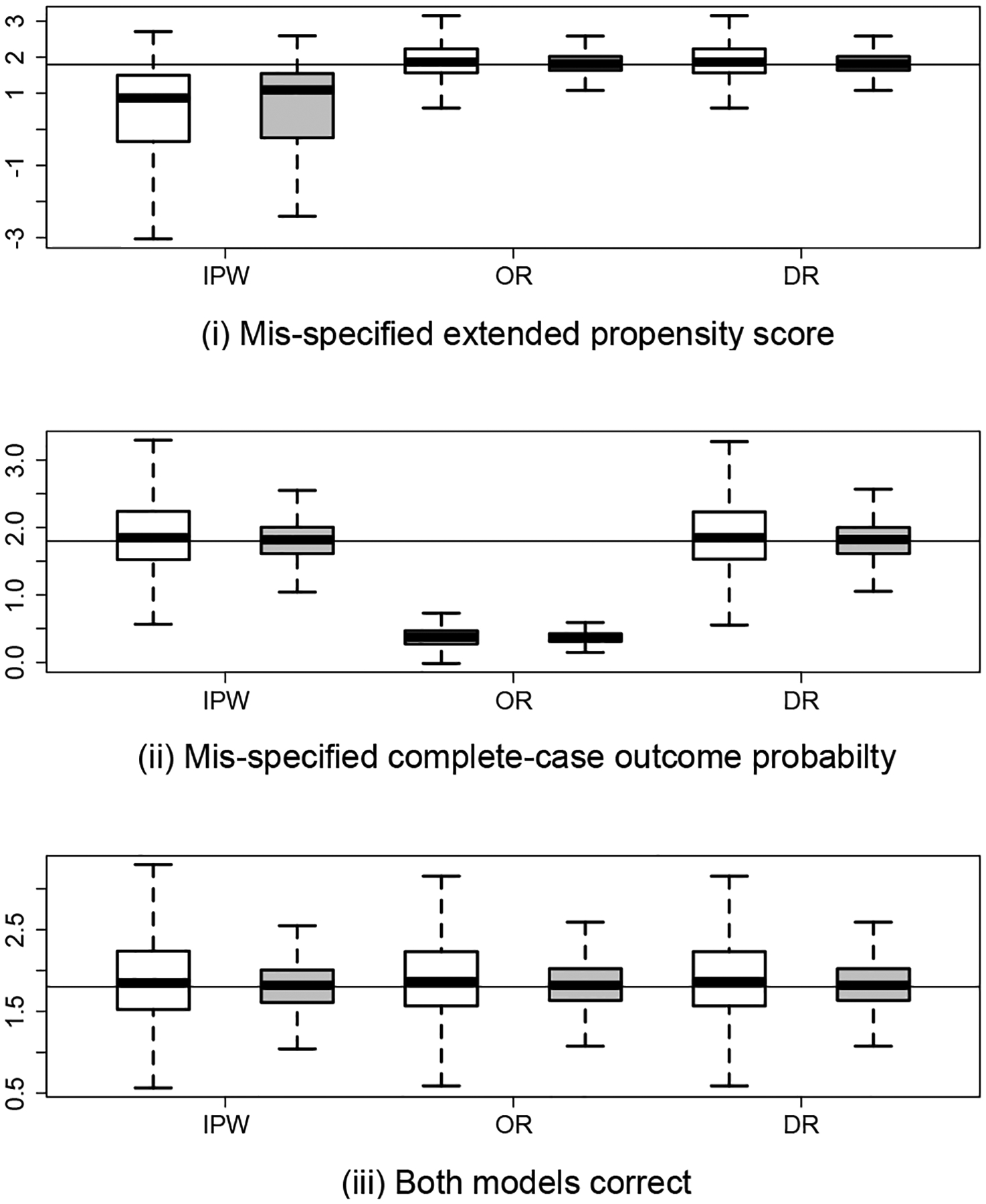
Boxplots of the inverse probability weighting (IPW), outcome regression (OR) and doubly-robust (DR) estimators of the selection bias parameter, for which the true value ζ₀ = 1.8 is marked by the horizontal lines. In each boxplot, white boxes are for n = 2000 and grey boxes are for n = 5000.

Figure 2:

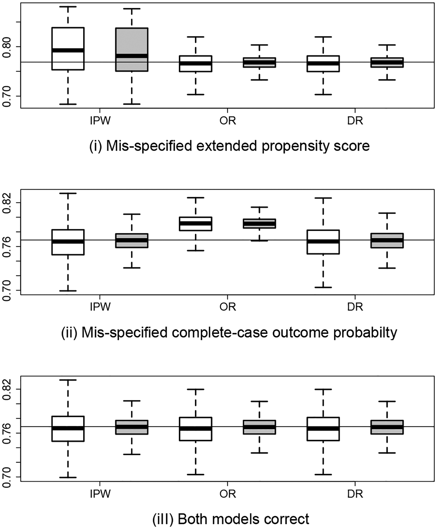
Boxplots of the inverse probability weighting (IPW), outcome regression (OR) and doubly-robust (DR) estimators of the outcome mean, for which the true value ϕ₀ = 0.769 is marked by the horizontal lines. In each boxplot, white boxes are for n = 2000 and grey boxes are for n = 5000.

Table 1:

Empirical coverage rates based on 95% Wald confidence intervals under three scenarios: (i) mis-specified extended propensity score, (ii) mis-specified complete-case outcome probability and (iii) both models are correct. In each scenario, the first row presents results for n = 2000 and the second row for n = 5000.

		ζ			ϕ
	IPW	OR	DR	IPW	OR	DR
(i)	86.4	95.4	95.4	81.3	95.2	95.2
	57.8	95.1	95.1	50.1	94.9	94.9
(ii)	95.0	0.0	94.4	95.1	65.6	95.2
	94.7	0.0	94.5	95.0	29.9	94.5
(iii)	95.0	95.4	95.4	95.1	95.2	95.2
	94.7	95.1	95.1	95.0	94.9	94.9

Under correct model specification, all estimators have negligible bias for ϕ₀ and ζ₀ that diminishes with increasing sample size, with empirical coverage near the nominal 95% level. In agreement with our theoretical results, the IPW and OR estimators are biased with poor empirical coverages when the extended propensity score or the complete-case outcome p.m.f. is mis-specified, respectively. The DR estimator performs well in terms of bias and coverage when either model is mis-specified but the other is correct. When all the models are correctly specified, the relative efficiencies of the efficient estimator compared to the DR estimator in estimation of ϕ₀ and ζ₀ are 0.88 and 0.65 respectively, based on Monte Carlo standard errors when n = 2000, demonstrating that substantial efficiency gain may be possible at the intersection submodel.

7. Applications

To illustrate the proposed IV approach, we obtained data from a household survey in Mochudi, Botswana to estimate HIV seroprevalence among adults adjusting for selective missingness of HIV test results. The data consist of 4997 adults between the ages of 16 and 64 who were contacted for the survey, out of whom 4045 (81%) had complete information on HIV testing. Of those who did not have HIV test results (R = 0), 111 (2%) agreed to participate in the HIV test but their final HIV outcomes are unknown, and 841 (17%) refused to participate in the HIV testing component. It is likely that refusal to participate in the survey when contact is established presents a possible source of selection bias.

Fully available individual characteristics from the survey include participant gender (X). Candidate IVs include interviewer gender (Z₁), age (Z₂) and years of experience (Z₃). These interviewer characteristics are likely to influence the response rates of individuals who were contacted for the survey, but are unlikely to directly influence an individual’s HIV status, given that interviewer deployment was determined at random prior to the survey. We implemented the proposed IPW, OR and DR estimators by making use of interviewer gender, age and years of experience as IVs. For IPW estimation, the missingness propensity score is specified as a linear main effects model with logistic link

$$\text{logit }P(R=1\mid X,Y,Z)={\omega }_0+{\omega }_{1}X+{\omega }_2{Z}_1+{\omega }_3{Z}_2+{\omega }_4{Z}_3+\zeta Y$$ (7.1)

where Y indicates HIV serostatus as our outcome of interest and the selection bias function is specified as α(x,y,z) = ζy. The posited missing data mechanism belongs to the separable logistic class, therefore the average HIV prevalence can be identified by Example 2. For OR estimation, we specified the regression model

$$\text{logit }P(Y=1\mid R=1,X,Z)={\theta }_0+{\theta }_{1}X+{\theta }_2{Z}_1+{\theta }_3{Z}_2+{\theta }_4{Z}_3.$$ (7.2)

Finally, the doubly robust estimator is implemented by incorporating both of the above two models. Because more than one IV was available, estimating equations U^IPW, U^OR and U^DR were solved using the generalized method of moments (GMM) package in R (Chaussé, 2010). Standard errors were obtained using the proposed sandwich estimator. For comparison, we also carried out standard complete-case analysis and standard IPW estimation assuming MAR given (x, z) under the propensity score model logit

$$\text{logit }P(R=1\mid X,Z)={\omega }_0+{\omega }_{1}X+{\omega }_2{Z}_1+{\omega }_3{Z}_2+{\omega }_4{Z}_3.$$ (7.3)

Results are presented in table 2.

Table 2:

Estimation for HIV seroprevalence (ϕ) and magnitude of selection bias (ζ) in Mochudi, Botswana with 95% Wald confidence intervals.

Estimator	$\widehat{\varphi }$	$\widehat{\zeta }$	$\widehat{\zeta }$ p-val
CC	0.214 (0.202, 0.227)	-	-
MAR IPW	0.213 (0.201, 0.226)	-	-
IV IPW	0.260 (0.175, 0.341)	−1.601 (−2.992, −0.210)	0.02
IV OR	0.241 (0.175, 0.307)	−0.757 (−1.889, 0.376)	0.19
IV DR	0.258 (0.174, 0.342)	−1.121 (−2.433, 0.191)	0.09

IV-based point estimates of HIV seroprevalence are 12.6 21.5% higher than the crude estimate of 0.214 (95% CI: 0.202–0.227) based on complete-cases only. Standard IPW (i.e. assuming MAR) produced similar estimates as complete-case analysis. Negative point estimates of the selection bias parameter ζ suggest that HIV-infected persons are less likely to participate in the HIV testing component of the survey, although this difference is statistically significant at 0.05 α-level only for IPW. The larger confidence intervals of the three IV estimators of ϕ₀ compared to those of the CC and MAR estimators are a more accurate reflection of the amount of uncertainty involving inferences about ϕ₀, since the CC and MAR estimators do not take into account the uncertainty about the underlying MNAR mechanism by assuming MCAR and MAR respectively, i.e. setting selection bias parameter ζ = 0. ${\widehat{\varphi }}^{\text{IPW}}$ and ${\widehat{\varphi }}^{\text{DR}}$ are close to each other. This comparison is useful as an informal goodness of fit test in that their similarity suggests that the missingness propensity score may be specified nearly correctly (Robins and Rotnitzky, 2001). In addition, by incorporating all possible pairwise interaction terms in the outcome logistic regression model (7.2) and therefore allowing it to be more flexible, the OR point estimate ${\widehat{\varphi }}^{\text{OR}}$ increases to 0.246 (95% CI: 0.179–0.314) and becomes closer to ${\widehat{\varphi }}^{\text{IPW}}$ and ${\widehat{\varphi }}^{\text{DR}}$.

References

- Chaussé P (2010). Computing generalized method of moments and generalized empirical likelihood with R. Journal of Statistical Software, 34(11):1–35. [Google Scholar]
- Chen HY (2007). A semiparametric odds ratio model for measuring association. Biometrics, 63(2):413–421. [DOI] [PubMed] [Google Scholar]
- Das M, Newey WK, and Vella F (2003). Nonparametric estimation of sample selection models. Review of Economic Studies, 70(1):33–58. [Google Scholar]
- Gill RD, van der Laan MJ, and Robins JM (1997). Coarsening at random: Characterizations, conjectures, counter-examples In Lin D and Fleming T, editors, Lecture Notes in Statistics. Springer-Verlag. [Google Scholar]
- Heckman JJ (1979). Sample selection bias as a specification error. Econometrica, 47(1):153–161. [Google Scholar]
- Heckman JJ (1997). Instrumental variables: A study of implicit behavioral assumptions used in making program evaluations. Journal of Human Resources, 32(3):441–462. [Google Scholar]
- Horton NJ and Laird NM (1998). Maximum likelihood analysis of generalized linear models with missing covariates. Statistical Methods in Medical Research, 8:37–50. [DOI] [PubMed] [Google Scholar]
- Horton NJ and Lipsitz SR (2001). Multiple imputation in practice: Comparison of software packages for regression models with missing variables. The American Statistician, 55(3):244–254. [Google Scholar]
- Kenward M and Carpenter J (2007a). Multiple imputation: Current perspectives. Statistical Methods in Medical Research, 16:199–218. [DOI] [PubMed] [Google Scholar]
- Kenward M and Carpenter J (2007b). Sensitivity analysis after multiple imputation under missing at random: A weighting approach. Statistical Methods in Medical Research, 16:259–275. [DOI] [PubMed] [Google Scholar]
- Li L, Shen C, Li X, and Robins JM (2013). On weighting approaches for missing data. Statistical Methods in Medical Research, 22(1):14–30. [DOI] [PMC free article] [PubMed] [Google Scholar]
- Lipsitz S, Ibrahim J, and Zhao L (1999). A weighted estimating equation for missing covariate data with properties similar to maximum likelihood. Journal of the American Statistical Association, 94:1147–1160. [Google Scholar]
- Little RJ and Rubin DB (2002). Statistical Analysis with Missing Data. Wiley. [Google Scholar]
- Lunceford J and Davidian M (2004). Stratification and weighting via the propensity score in estimation of causal treatment effects: A comparative study. Statistics in Medicine, 23:2937–2960. [DOI] [PubMed] [Google Scholar]
- Manski CF (1985). Semiparametric analysis of discrete response: Asymptotic properties of the maximum score estimator. The Econometrics Journal, 27(3):313–333. [Google Scholar]
- Miao W, Ding P, and Geng Z (2014). Identifiability of normal and normal mixture models with nonignorable missing data. Journal of the American Statistical Association, Submitted. [Google Scholar]
- Moreno-Betancur M and Chavance M (2013). Sensitivity analysis of incomplete longitudinal data departing from the missing at random assumption: Methodology and application in a clinical trial with drop-outs. Statistical Methods in Medical Research, doi: 10.1177/0962280213490014. [DOI] [PubMed] [Google Scholar]
- Neugebauer R and van der Laan M (2005). Why prefer double robust estimators in causal inference? Journal of Statistical Planning and Inference, 129:405–426. [Google Scholar]
- Newey WK (2009). Two-step series estimation of sample selection models. The Econometrics Journal, 12(S1):S217–S229. [Google Scholar]
- Newey WK, Powell J, and Walker J (1990). Semiparametric estimation of selection models: some empirical results. The American Economic Review, 80(2):324–328. [Google Scholar]
- Potthoff RF, Tudor GE, Pieper KS, and Hasselblad V (2006). Can one assess whether missing data are missing at random in medical studies? Statistical Methods in Medical Research, 15:213–234. [DOI] [PubMed] [Google Scholar]
- Puhani P (2000). The heckman correction for sample selection and its critique. Journal of Economic Surveys, 14(1):53–68. [Google Scholar]
- Robins J, Rotnitzky A, and Scharfstein D (2000). Sensitivity analysis for selection bias and unmeasured confounding in missing data and causal inference models In Halloran E and Berry D, editors, Statistical Models in Epidemiology, the Environment, and Clinical Trials. Springer-Verlag. [Google Scholar]
- Robins JM and Ritov Y (1997). Toward a curse of dimensionality appropriate (coda) asymptotic theory for semi-parametric models. Statistics in Medicine, 16:285–319. [DOI] [PubMed] [Google Scholar]
- Robins JM and Rotnitzky A (2001). Comment on “inference for semiparametric models: Some questions and an answer”. Statistica Sinica, 11:920–936. [Google Scholar]
- Robins JM, Rotnitzky A, and Zhao LP (1994). Estimation of regression coefficients when some regressors are not always observed. Journal of the American Statistical Association, 89(427):846–866. [Google Scholar]
- Rotnitzky A and Robins J (1997). Analysis of semiparametric regression models with non-ignorable non-response. Statistics in Medicine, 16:81–102. [DOI] [PubMed] [Google Scholar]
- Rotnitzky A, Robins JM, and Scharfstein DO (1998). Semiparametric regression for repeated outcomes with nonignorable nonresponse. Journal of the American Statistical Association, 93:1321–1339. [Google Scholar]
- Rotnitzky A, Scharfstein DO, Su T, and Robins JM (2001). Methods for conducting sensitivity analysis of trials with potentially non-ignorable competing causes of censoring. Biometrics, 57:103–113. [DOI] [PubMed] [Google Scholar]
- Roy J (2003). Modeling longitudinal data with nonignorable dropouts using a latent dropout class model. Biometrics, 59:829–836. [DOI] [PubMed] [Google Scholar]
- Rubin DB (1987). Multiple Imputation for Nonresponse in Surveys. John Wiley & Sons. [Google Scholar]
- Schafer J (1999). Multiple imputation: a primer. Statistical Methods in Medical Research, 8(1):3–15. [DOI] [PubMed] [Google Scholar]
- Scharfstein DO, Daniels MJ, and Robins JM (2003). Incorporating prior beliefs about selection bias into the analysis of randomized trials with missing outcomes. Biostatistics, 4(4):495–512. [DOI] [PMC free article] [PubMed] [Google Scholar]
- Scharfstein DO, Rotnitzky A, and Robins JM (1999). Adjusting for nonignorable dropout using semiparametric nonresponse models (with discussion). Journal of the American Statistical Association, 94:1096–1146. [Google Scholar]
- Tchetgen Tchetgen E (2009). A simple implementation of doubly robust estimation in logistic regression with covariates missing at random. Epidemiology, 20(3):391–394. [DOI] [PubMed] [Google Scholar]
- Tchetgen Tchetgen EJ, Robins JM, and Rotnitzky A (2010). On doubly robust estimation in a semiparametric odds ratio model. Biometrika, 97(1):171–180. [DOI] [PMC free article] [PubMed] [Google Scholar]
- Tchetgen Tchetgen EJ and Wirth K (2013). A general instrumental variable framework for regression analysis with outcome missing not at random. Harvard University Biostatistics Working Paper Series, Working Paper 165. [DOI] [PMC free article] [PubMed] [Google Scholar]
- Tsiatis AA (2007). Semiparametric Theory and Missing Data. Springer. [Google Scholar]
- van der Laan M and Robins JM (2003). Unified Methods for Censored Longitudinal Data and Causality. Springer-Verlag. [Google Scholar]
- Vansteelandt S, Rotnitzky A, and Robins JM (2007). Estimation of regression models for the mean of repeated outcomes under non-ignorable non-monotone non-response. Biometrika, 94:841–860. [DOI] [PMC free article] [PubMed] [Google Scholar]
- Varadhan R and Gilbert P (2009). BB: An R package for solving a large system of nonlinear equations and for optimizing a high-dimensional nonlinear objective function. Journal of Statistical Software, 32(4):1–26. [Google Scholar]
- Wang S, Shao J, and Kim JK (2014). An instrumental variable approach for identification and estimation with nonignorable nonresponse. Statistica Sinica, 24:1097–1116. [Google Scholar]
- Winship C and Mare R (1992). Models for sample selection bias. Annual Review of Sociology, 18:327–350. [Google Scholar]
- Wooldridge J (2010). Economic Analysis of Cross Section and Panel Data. MIT press. [Google Scholar]
- Wu M and Carroll R (1988). Estimation and comparison of changes in the presence of informative right censoring by modeling the censoring process. Biometrics, 44:175–188. [PubMed] [Google Scholar]
Associated Data
This section collects any data citations, data availability statements, or supplementary materials included in this article.