Abstract
Background
Assessing why the spread of the COVID‐19 virus slowed down in many countries in March through to May of 2020 is of great significance. The relative role of restrictions on behaviour (“lockdowns”) and of a natural slowing for other reasons is difficult to assess when mass testing was not widely done. This paper assesses the evolution of the spread of the COVID‐19 virus over this period when there was no data on test results for a large, random sample of the population.
Method
We estimate a version of the susceptible‐infected‐recovered model applied to data on the numbers who were tested positive in several countries over the period when the virus spread very fast and then its spread slowed sharply. Up to the end of April 2020, test data came from non‐random samples of populations who were overwhelmingly those who displayed symptoms. Using data from a period when the criteria used for testing (which was that people had clear symptoms) was relatively consistent is important in drawing out the message from test results. We use this data to assess two things: how large might be the group of those infected who were not recorded and how effective were lockdown measures in slowing the spread of the infection.
Results
We find that to match data on daily new cases of the virus, the estimated model favours high values for the number of people infected but not recorded.
Conclusions
Our findings suggest that the infection may have spread far enough in many countries by April 2020 to have been a significant factor behind the fall in measured new cases. Government restrictions on behaviour—lockdowns—were only one factor behind slowing in the spread of the virus.
What’s known
While there are estimates of the spread of the virus, they cover a very large range and are highly uncertain.
What’s new
We use a technique which pays great attention to unrecorded cases to estimate the spread of the virus and its contribution to the slowing spread in the Spring of 2020.
1. INTRODUCTION
There is significant uncertainty about the degree to which the novel coronavirus (COVID‐19) has spread. This is particularly true over the period when, in many European countries, those testing positive for the infection rose fast and subsequently slowed markedly. Over the period between February and May 2020, in most countries, there was no mass testing. Although testing capacity did rise, it did so along with the rise in infections and testing was largely confined to those with symptoms. This has very significant policy implications—Stock 1 showed that different policies aimed at controlling the virus can have very different effects on the numbers who become infected and show symptoms depending on the proportion of those who are asymptomatic. It is those with symptoms who are at risk of death from the virus and so the relative size of the populations of symptomatic to asymptomatic among the infected is of enormous significance to welfare, including mortality rates, and to policy. 2
The degree of uncertainty about that asymptomatic rate is large enough to mean that neither 0.3 nor 0.9 is outside the range of plausible values, although the implications of those two numbers are very different. Li et al 3 estimated that 86% of all infections were undocumented prior to the Wuhan travel shutdown (on 23 January 2020). In contrast, estimates based on infections among passengers on the cruise ship Diamond Princess put the proportion of asymptomatic (or near asymptomatic) cases at around 50%. Manski and Molinari 4 reported enormous ranges for the possible values of the infection rates in Illinois, New York and Italy. As of 6 April 2020, these ranges were estimated as [0.001, 0.517], [0.008, 0.645] and [0.003, 0.510], respectively.
While large‐scale testing of a random sample of the population would narrow the range of plausible values for the asymptomatic proportion of the infected, 1 such testing did not come in many countries until after the end of April. That makes it harder to judge now why the spread of the infection seemed to slow so sharply in March and April. In most countries, including the United States and the United Kingdom, testing up to the end of April 2020 was concentrated on those who displayed symptoms or were at high risk; it was certainly not random. However, testing capacity did rise strongly over this period; in the United Kingdom, testing went from under 10 000 a day in early March to almost 100 000 a day by early May (according to Office for National Statistics data). Until late April, UK testing was overwhelmingly done in hospitals on those who displayed symptoms of the virus. So called “pillar 2” tests have subsequently increased greatly and are carried out on the wider population outside of hospitals.
In this paper, we implement a version of the susceptible‐infected‐recovered (SIR) model to estimate the numbers infected from data on the non‐random sample of those tested. We use data from the United Kingdom, where relatively few of those showing no symptoms had been tested up to the end of April 2020, to provide estimates of the spread of the virus over that period.
We also apply the model to the United States, Italy, Spain, France and Sweden. In doing so, we allow the estimated parameters of the model to vary thereby accounting for a range of factors that are different between countries and which are likely to affect the spread of the virus. Population density, climate, age structure, working patterns, family structure and living arrangements are likely to vary across countries and have an impact on how the virus is transmitted. Our statistical technique allows for these factors that differ between countries, but which are relatively stable within countries over the months we focus on.
The results for these countries are similar to the United Kingdom—the numbers of those untested but infected that seems to best fit the data are very high; far higher than is estimated based on the limited amount of results from more widespread testing which went beyond those who showed symptoms. But other studies using UK data do find evidence of wider spread of the virus in March and April. An Oxford University research team used death data to estimate the proportion of the population who might have built up some form of immunity before the UK lockdown was introduced in mid‐March. They put that fraction at around 60%. 5 Stedman et al 6 used data on differences in the spread of the infection across English regions to assess how many might have been infected and put that fraction at similarly high levels, which is similar to the study by Delius et al 7
2. THE MODEL
We use a version of the SIR model which closely follows the model used by Stock. 1 At each point in time, the population is made up of three distinct groups: those who are currently infected (); those who are susceptible () and those who have recovered (). We assume a constant population and that the death rate is low enough to mean that this is reasonable. At each point in time, only some fraction of those infected are tested and show a positive result. Over the period we consider, it is likely that many of those who were infected but not tested had mild, or no, symptoms. We use the symbol to denote the fraction of those infected who are not recorded. There is some evidence that the degree to which the asymptomatic are infectious may be different from those who have symptoms, 8 but we will initially assume that the transmission rates are the same for those infected, whether tested or not. We denote the number of people infected at time by . We distinguish within this group between those who have tested positive (denoted ) and those who were not tested or incorrectly tested negative () such that . (We use the subscripts s and a for these groups because those who were tested were disproportionately those with symptoms while those who were infected but not tested were likely to have had a higher proportion of the asymptomatic). The evolution of , and in discrete time is given by the dynamic system:
| (1) |
| (2) |
| (3) |
where is the change in the population of the susceptible, is the total population, is the transmission rate of the virus at a time (the mean number of people an infectious person will infect per unit time) and is the rate of recovery. The initial infection rate over the infectious period, the reproduction number, is defined as . Initially, we shall assume that is a constant so that
| (4) |
and
| (5) |
The number of new cases at time () can be calculated as follows:
| (6) |
New cases are the sum of the change in the number of outstanding cases plus the numbers recovered. The number of new recorded cases () is as follows:
| (7) |
The strategy that we pursue is to use the data on the numbers of new cases who test positive for the virus. We then seek the values of the parameters of the model—and in particular —that give a predicted that matches the data. We use data on the numbers of those who test positive (in the United Kingdom and in other countries) as the variable we are trying to match; other studies 5 , 9 use the number of deaths. There would seem to be significant ambiguity over assignment of the cause of death to the virus, perhaps more than over whether a positive test is reliable or not.
We use data on tests up the end of April 2020 by which time nearly 500 000 had been tested in the United Kingdom and around 175 000 had tested positive (according to data from the Office of National Statistics). It is over this period that new cases testing positive first rose dramatically and then began to fall sharply a few weeks after lockdown began. It is the main purpose of this paper to identify the contribution to this slowdown of behavioural changes and of the natural dynamics of infections arising from a shifting stock of those who have been infected. This is why we focus on the February–April period.
To implement the estimation of the model, we need to make assumptions about the transmission rate of the virus and the recovery rate . The transmission rate will not have been constant because of policy measures introduced to slow the spread of the infection and because of behavioural changes that were happening even in the runup to the lockdown. In the United Kingdom, “lockdown,” which began on March 23, was strict and social distancing was already happening just before this date; both would have likely brought down significantly. Similar policies were adopted at various times in March 2020 in other countries. We assume a constant value of before the lockdown date (of ), followed by a gradual reduction in the value after this date to simulate the effect the measures have on transmission. The initial value of is derived from the value of the initial reproduction rate and the recovery rate , using the relation . We try all values for an initial reproduction rate ranging from 2.2 up to 3.9 at intervals of 0.005. We try three values of the recovery rate implied by half lives of the period of infectiousness—that is the number of days it takes for half an initial number of infected people to recover—of 4 days, 6 days (as used by James 1 ) and 8 days. The corresponding three values of are 0.159, 0.109 and 0.0833.
We assume that after the lockdown date there is a lag until the value of starts to change from . The lag is between the lockdown measures starting and the impact on the numbers testing positive for the virus. That lag reflects several distinct factors: it must include the lag in the impact on new infections, the lag before symptoms show, the lag before testing the symptomatic and finally the lag before results are known and recorded in the daily measure. We not only set the overall lag at 14 days, but also assess sensitivity of results to shorter lags in part because social distancing was already happening just before lockdown. After this lag, decays exponentially towards a value of , the post‐lockdown asymptotic . The time path for can be expressed as follows:
| (8) |
where is the lockdown time plus the 14‐day lag period and is the speed of adjustment in after lockdown measures begin to take effect. We assume that once the lockdown does begin to affect numbers testing positive it quite quickly reaches its full effectiveness, bringing the transmission rate down so that half of its long run impact on comes through in 3 days, implying that .
For given values of , and , we search for the values of the two free parameters— and —so as to maximise the fit of the model. We choose those two free parameters to minimise the root mean squared (RMS) deviation between the daily data on the numbers of new positive tests for the virus and the model prediction of that number (). The parameters we fit are a measure of how effective the lockdown is in bringing down the infection rate (measured by how much lower is relative to ) and the ratio of those infected but not tested to the total population of the infected ().
These key parameters are the ones which best match each country's data on test results. Separate estimation of these parameters for each country allow for cross‐country differences in characteristics that might affect the spread of the virus.
3. SENSITIVITY TO KEY ASSUMPTIONS AND CALIBRATION
Before showing results, we stress that our model relies on a number of key assumptions.
In its simplest version, we assume is a constant but we then allow for it to vary with changes in testing capacity. Overall, relatively few in the United Kingdom with no symptoms had been tested up to the end of April 2020. For the other countries, we are also focusing on a period over which testing was largely confined to those with clear symptoms. This is important because it means that the results from tests over this period can be expected to reflect the spread of the virus much better than if we extend the period to one where testing became far more widely available to those with few or no symptoms. Nonetheless there was some variability in the criteria for testing over the period up to the end of April 2020. In the United Kingdom, testing was ramped up strongly in late April and as it was, the ratio of daily positive tests to total tests fell. We take account of the possible impact of that below but first continue with the assumption of a fixed .
For the United Kingdom, the model is initialised on data from the 31st of January, the date on which the first non‐zero value of positive test cases is recorded. At this time, testing was only applied to those who had travelled to certain regions of China and presented with symptoms and therefore data in the first week or so may not be fully representative of all symptomatic cases.
We rely on estimates of and of to generate a value for . There is considerable uncertainty about both. At the lower end of the ranges of values used in simulations are those chosen by Ferguson et al, 8 who assume a value of 2.4, and Lourenco et al 5 who take figures centred around 2.25 or 2.75. Stock, 1 who draws on estimates using data from Wuhan, uses a much higher figure for simulations with a pre‐shutdown value for of 3.8. The range of estimates of from several studies is between 2.2 and as high as 3.9. A team at the London School of Hygiene and Tropical Medicine found 11 published estimates of R0 for COVID‐19, which averaged 2.68 with a standard deviation of 0.57 (see Paul Taylor, London Review of Books, May 2020, vol 42, no 9). The range we use for simulations is 2.2‐3.9—values outside this range gave a poor fit to the data for all countries we analysed for any values of the other parameters. For our estimate of , we assume the half‐life of the infection as days and therefore that satisfies the . We take as 4, 6 or 8 days—a range which encompasses those used in several studies.
As noted above, we assume that once lockdown begins beta is reduced so that it declines asymptotically towards a value that would then be maintained as long as the lockdown remains in place ( in our equations). Our choice of the speed with which β declines towards its steady‐state value, after the initial lag, is such that the transition is fairly rapid, corresponding to a half‐life of 3 days ().
The data we try to fit is the number of new infections recorded. Testing of people with no symptoms was (up to late April 2020) relatively small scale in the countries we analyse and to a large extent limited to those at high risk. We use a grid search to find the values of the two unknown and free parameters ( and ) to minimise the root mean squared deviation between the observations and (), given the choice of other parameters.
4. RESULTS
Figure 1 shows the data on new cases of those testing positive for the virus in the United Kingdom. The data start on January 31. The data are from the Office for National Statistics. (The spike in reported new cases on 11 April 2020 coincides with an expansion in testing capacity.)
FIGURE 1.
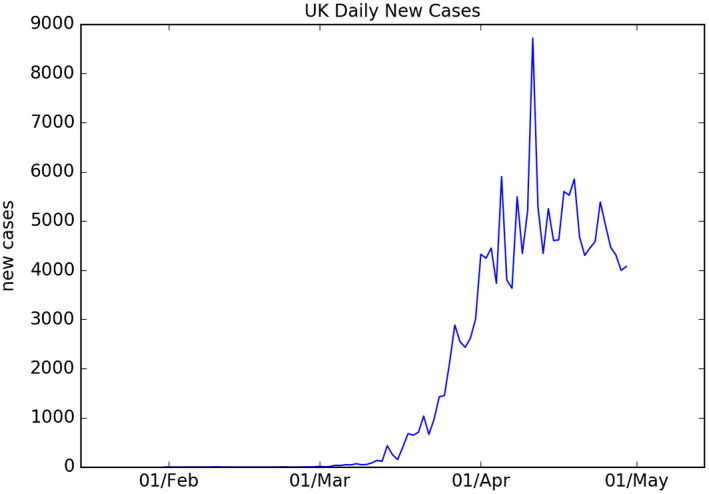
Time series of daily new positive COVID‐19 cases recorded in the UK between 31 January and 30 April 2020
Figure 2 shows the best fit of the model when we set the half‐life of the infection to 6 days (). The best fit for this value of was when and and are 0.1928 and 0.996, respectively. These values imply that the transmission rate started to turn down sharply by the end of first week of April, some 2 weeks after the lockdown began. The value for is very high—implying that, in the period up to the end of April, there were around 250 people with the infection for every person who tested positive. If that were true, then by April 20 around 120 000 had tested positive for the virus (and the great majority of whom had shown symptoms) close to 45% of the UK population might have had the virus.
FIGURE 2.
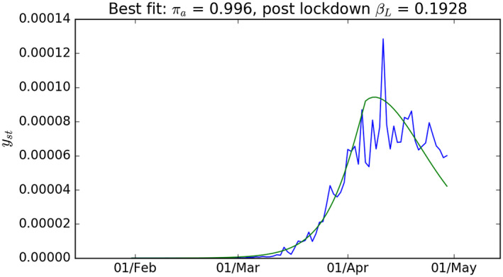
Results from the free parameter optimisation of the model with γ = 0.109. UK new case data from Figure 1 given as a proportion of total population (blue) and model simulation for γst that gives the best fit to the UK data (green)
Figure 3 shows the RMS error of the model for all combinations of parameters and . The area on the far right of the figure shows the fit of the model in cases where the lockdown had limited effect (ie is little different from ). The model fits the data very poorly in this region—as illustrated by the darker shading which reflects a high value of the RMS error—suggesting the lockdown had a significant impact.
FIGURE 3.
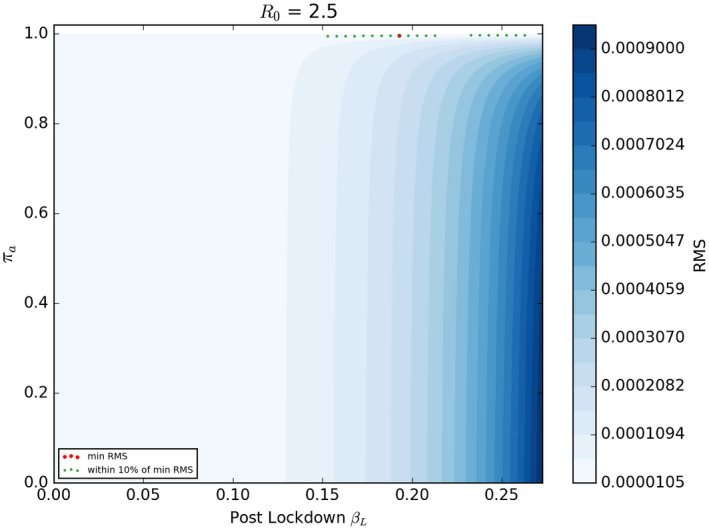
RMS difference between UK new case data and γst for all combinations of πa and βL for simulations with γ = 0.109. The combination that gives the lowest RMS value (the best fit) is shown as a red dot. The combinations that give and RMS value within 10% of the minimum RMS are shown in green
Figure 4 shows the model fit to the UK data when we set the half‐life of the virus at 8 days (). The best fit here was with a value of R0 of 2.95 and and of 0.1598 and 0.996, respectively. Once again the best fit value of is very high and it implies that approximately 45% of the UK population may have been infected by late April. Figure 5 shows the parameter combinations that have a goodness of fit within 10% of the best pair of values; once again these are bunched fairly closely around the best fit values with all such pairs generating a value of close to 0.996. The fit of the model deteriorates so sharply when we set the half‐life of the virus to be only 4 days that we do not show those results. The parameter space in Figure 5 shows the best fit parameters (red dot) and also the parameter combinations that generate a RMS error within 10% of the best value. This is illustrative of the degree of uncertainty around the best fit values of the two parameters.
FIGURE 4.
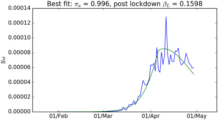
Like Figure 2 with γ = 0.0833
FIGURE 5.
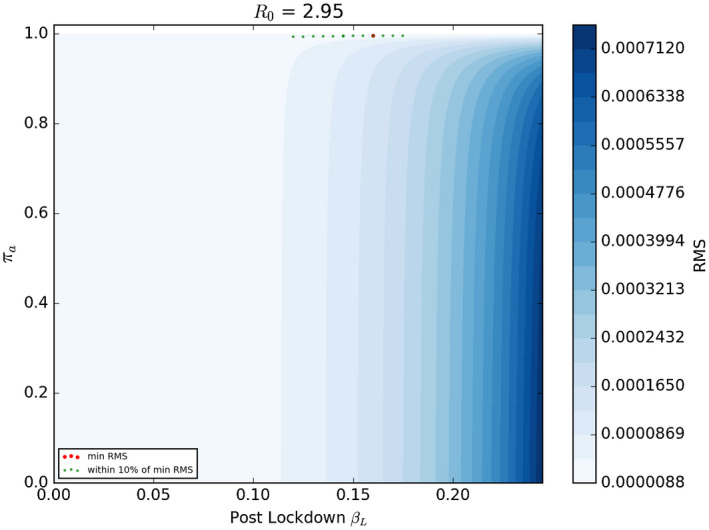
Like Figure 3 with γ = 0.0833
However, it is difficult to construct precise confidence regions around the best‐fit parameter estimates. In the appendix, we discuss robust methods for calculating confidence intervals on these parameter estimates. Using these intervals, our results suggest that one could reject the hypothesis that is below 0.9 at the 10% level of statistical significance, but not at higher levels. In short, one cannot be very sure that the main reason why test cases of those newly infected turned down was because a large fraction of the population had already been infected (very high ) rather than a low value of (a very effective lockdown). Nonetheless, as we describe in more detail below, we consistently find the best fit for the data (for both the United Kingdom and other countries) is for a very high value of .
5. ALLOWING TO VARY WITH TESTING CAPACITY
Testing capacity rose significantly in the United Kingdom particularly in the last 2 weeks of April 2020. It is possible that along with this rise in testing capacity there was a significant change in the proportion of new infections that were recorded as positive tests; this would invalidate the assumption of a constant . However, the fact that test capacity rose significantly need not mean that recorded cases rise as a proportion of all infections. If test capacity simply rises in line with new cases of the infection, may well be approximately constant.
We assess whether the evidence suggests that varies significantly with testing capacity. We do so by allowing for the value of to systematically vary with the fraction of test results that are positive. The idea is simple: if testing capacity has substantially moved ahead of the rise in new infections, then more people who would not have been tested when capacity was used largely on those with clear symptoms will now be tested. As this happens, the fraction of tests which are positive is likely to decline along with a fall in the fraction of new infections that are not recorded. We now allow the value of to vary with , the fraction of positive tests to total tests at time . We allow for a flexible non‐linear form of this relation. This is given as follows:
| (9) |
where is at time , that is the fraction of unrecorded new cases to all new infections. b 1 and b 2 are the parameters we estimate to best fit the data. The natural log is denoted ln. We expect to be non‐negative. If is positive then as the proportion of positive tests to total tests falls (which would happen if testing capacity rises much faster than the numbers becoming infected) the fraction of unrecorded new cases of the virus also falls. A special case of (9) is when b 2 = 0 and is constant, the assumption we made in estimates shown in the previous section. Now we carry out a grid search over values , and to minimise the RMS error of the model. We calculate the series as the ratio of daily new cases to daily total tests using data from the Office for National Statistics.
When we estimate these parameters, we find that the value of that best fitted the data was 0. At first glance, this seems surprising because testing capacity was clearly not constant. But what matters is testing capacity relative to the scale of infection which was likely much less variable than the number of tests undertaken. Nonetheless there are small positive values of which fit the data almost as well as and which give notably different variations in . Figure 6 illustrates the model when we set . In this case, the fit of the model deteriorates by just over 25% relative to when and when is constant—though it could not be rejected at standard significance levels. The implied path of is far from constant and significantly lower than when we assume it is a constant (Figures 3 and 5). This value of would imply that in April 2020 when was around 0.93 there were around 14 unmeasured infections for every measured one—a far lower ratio than if was at 0.99 or higher when the unrecorded cases would be at least 100 times as great as the recorded cases. At values of above 0.1, the quality of fit of the model deteriorates significantly and such values can be rejected using similar tests to those outlined in Appendix A.
FIGURE 6.
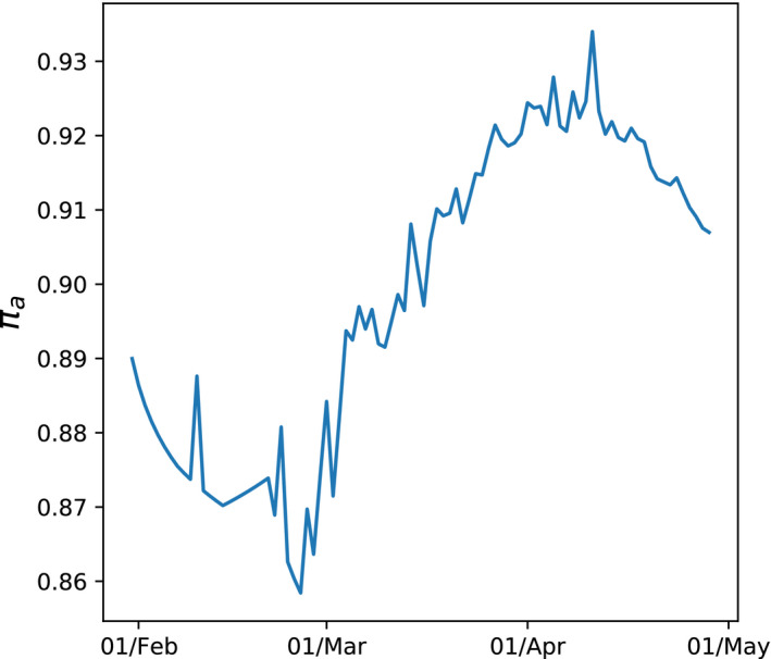
Time varying estimate of πa when b2 =0.1
6. RESULTS FOR FRANCE, UNITED STATES, ITALY, SPAIN AND SWEDEN
We described above that the model that best fits the UK data was one with constant . We estimate this constant model for other countries where up to the end of April 2020 testing had largely been confined to those with symptoms or those at high risk. Data for those testing positive comes from the Johns Hopkins data bank. Dates at which measures to reduce the spread of the virus became severe (the lockdown date) were taken from the Blavatnik Centre at Oxford University which has constructed an index of the severity of measures. We choose the date at which that index rises most sharply to be our starting date for lockdown measures. The dates used are outlined in Table 1. For the United States, the date is problematic because actions vary substantially across states.
TABLE 1.
Lockdown dates for various countries used for simulations
| Country | Lockdown date |
|---|---|
| France | 16 March |
| Spain | 10 March |
| Italy | 23 February |
| Sweden | 19 March (partial lockdown) |
| USA | 16 Mar (localised lockdown) |
The estimated impact of the lockdown measures and of the speed of the spread of the virus pre‐lockdown, are estimated separately for each country. Since lockdown measures differ significantly across countries (mild in Sweden; severe in France), we expect estimates of the difference between and could be substantial across countries. More generally, country characteristics will likely have influenced the path the virus took. The statistical technique we use allows for this. That is because the parameters that we estimate for the spread of the virus are estimated separately for each country so that the impact of cross country differences that affect the spread of COVID‐19 (like population density, age structure, working patterns, living conditions, etc) are already allowed for. We chose parameters at the level of the country to best fit the spread of the virus in that country. We also allow the estimated effectiveness of lockdowns (which might also depend on density, travel patterns, labour force participation, etc) to vary across countries and it is estimated in a way that best fits the progress of the virus in each country.
Figure 7 show the fit of the model for each country. The most striking result is that the values of that best fit the national data on positive tests for the virus are consistently at very high levels—generally around 0.995 (though lower for the United States). As with the UK results, taken at face value this would mean that there are 200 or so people who have had the virus but whose infection was not recorded for every recorded case.
FIGURE 7.
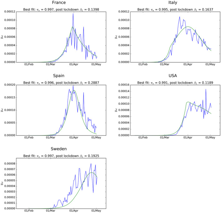
Estimated best fit model for recorded new cases in each country. R0 values used are 2.95 (France); 3.30 (USA); 3.90 (Italy); 3.90 (Spain); 2.50 (Sweden)
But what is equally striking, and much less reassuring, is that these best‐fit estimates for are much higher than those implied by other methods for assessing the spread of the virus up to April 2020. Some cross country studies based on deaths associated with the virus (eg Flaxman et al 9 ) suggest that only between 5% and 10% of populations in the countries studied here have been infected. Results from tests for antibodies in samples of the population from a range of European countries suggest a similar proportion of the population has been infected. However, it is possible that serology testing for past COVID‐19 infection based on the presence of antibodies are not picking up cases where the infected had very few symptoms and not identifying others who are nonetheless not susceptible to the virus. There is evidence that such tests are not reliable. 10
7. INTERPRETATION, CAVEATS AND IMPLICATIONS
Our estimates suggest that in the United Kingdom, and in the other countries whose data we have analysed, there were, in the period up to the end of April, very many unrecorded infections. For the United Kingdom, the best fit of the model implies that there were as many as 200 or so unrecorded infections for every recorded case. If that were true, then much of the decline in the spread of the virus would have been attributable to a degree of immunity having built up in the population. Our model also implies that R fell from 2.95 in early February to just under 1 by the end of April. Our estimate of the parameter implies that a significant part of this was because of behavioural changes which reduced by enough to bring R down to approximately 1.9. But a slightly larger reduction in R came from the build‐up in immunity implied by the estimate of . At face value, our results suggest that both factors played a major role in bring down the spread of the infection sharply by the end of April.
But why should results of the SIR model designed to fit the UK test data (and which also seem to best fit data from Italy, Spain, France, Sweden and the United States) suggest a much higher rate of the spread of the virus than antibody test data from countries that have done more widespread (closer to random) testing including the United Kingdom and Spain? One answer is purely mechanical: if one wants to fit a model that tracks the data on positive tests it must be one where the number of infections rises very fast early on (a relatively high and ). Is it possible that we have made assumptions which force the model to explain much more of the slowdown in new positive test cases by a fast rise in the immune population (which implies a very large group have had the virus with few symptoms) rather than attribute it to a very effective lockdown? One factor may be significant: we have assumed a 14‐day delay between the start of the lockdown and its beginning to affect the rate of new positive tests for the virus. If that lag were much smaller, more of the turnaround in new cases might be attributed to the lockdown and correspondingly less to a rise in mass immunity. But, in fact, when we halve the lag between the start of the lockdown and its effect on we still find that the value of that best fits the data remains very close to 1.
There is, however, one assumption that does have a significant impact on our results. This is that is the same for all infected people, whether recorded or not. It is likely that there are more asymptomatic people amongst the unrecorded and it is possible that the spread of the virus for this group is lower than that for the symptomatic. If the rate at which the asymptomatic infect people is significantly lower than for the symptomatic, the best way for our SIR model to explain the UK data is to have a much lower number of unrecorded cases (). If the transmission rate of the unrecorded is one half that of the recorded, but the weighted average of the two keeps the overall as it was, falls to approximately 0.5. But, the fit of the model deteriorates and the RMS error is around 16% higher than the lowest value obtained in simulations with identical transmission rates.
There is limited evidence that the transmission of the virus is weaker for those with few symptoms. 3 But, it is clear that it matters for modelling the spread of the virus. 11 The influential Imperial College study 8 report does assume a lower asymptomatic transmission rate (by 50%). The analysis of Gupta and her team, 5 designed to explain the early spread of the virus in the United Kingdom, appears to assume a common transmission rate amongst the infected. That study suggested that the asymptomatic were a very high proportion of the infected and that the virus had spread very widely by early March. Our study suggests that estimates of the spread of the virus that best account for the data are sensitive to whether the transmission rate is assumed to be the same for asymptomatic and symptomatic groups.
We have found that when trying to match data in the period up to the end of April on the recorded cases of the virus our model appears to favour high values of (the unrecorded proportion of the total infected people). This is a consistent finding across a number of scenarios where we vary the mean transmission rate, the recovery rate and lockdown measures. It is only when the transmission rate for the unrecorded is much lower than for the (largely symptomatic) recorded cases that the best fitting estimate of is reduced. These two facts lead to two conclusions: First, that previous estimates of near 0.9, 3 or even higher, are consistent with versions of a simple SIR model designed to track results of tests for the virus in the United Kingdom and other countries; but we do not make the stronger claim that the evidence clearly proves such a high value. Second, that reliable modelling of the evolution of the spread of the virus requires accurate measurement of transmission rates for symptomatic and asymptomatic groups and is sensitive to whether these are different.
In all the countries whose data we analysed, the best fit to that data suggests that there have been a very large number of unrecorded infected cases for each recorded case. But the data by no means overwhelmingly reject the hypothesis of a value of lower by enough to mean that the main cause of the slowdown (and then reversal) in the arrival of new positively tested cases of the virus in March and April were the measures taken to curb it. But our results suggest that a factor that several other studies simply ignore—namely that the virus had spread fast enough to itself generate substantial immunity by the spring of 2020 which slowed the spread—was indeed significant. While the results do not show that a degree of immunity clearly was more powerful than lockdowns, the results (which are consistent across countries) do show that it is likely to have been a significant factor.
APPENDIX A.
CONFIDENCE INTERVALS FOR PARAMETER ESTIMATES
Under restrictive assumptions, the parameter space within which the standard error of the model is within 10% of the best fit would very likely contain the true parameter values. Standard tests based on the assumption of independent and normally distributed residuals between data and the fit of the model would imply a small chance of parameters lying outside this area. The statistic s, where is the unrestricted minimum residual sum of squares, is the sum of squared residuals at some other restricted value of the parameters and is the sample size (in this case number of days we run the simulation over) would follow a distribution if all the ideal assumptions for OLS estimation were satisfied. At a value of 90 the 1% confidence region for that statistic with two estimated parameters would include only values where the standard error of the model were within around 5.2% of the best value. An F version of this test, based on the statistic and where , would imply a 1% confidence region including parameters generating a standard error no more than around 5.6% above the best fit value. However, the conditions for these parametric methods to be a reliable guide to the uncertainty over parameter estimates do not hold: the model is highly non‐linear and the values of state variable used to generate predictions of —that is and —are themselves generated using the estimated parameters. To overcome this, we use a simple bootstrap technique to judge confidence intervals for the parameters. We take the set of squared residuals between data and the model using the best fit parameter values and also construct T squared residuals at some other point in the parameter space we wish to compare to. We construct a pooled square residual dataset by combining the two sets (giving values), from which we randomly draw 2 samples (without replacement) each of size T. For each pair of samples we calculate the mean difference between them. We repeat this 10 000 times and construct the frequency distribution of outcomes. We then calculate where the actual mean difference in squared residuals between the two parameter estimates is in this sample distribution. We can construct such a distribution by taking the point in an RMS grid (Figure 5) which gives the best fit and comparing the residuals to another point in parameter space defined by ( and ). This value of is chosen as it minimises the RMS for . The mean of the distribution of constructed differences in sums of square residuals is very close to zero (its expected value) and the actual difference in squared residuals based on the two sets of parameter estimates lies at around the 91st percentile of the distribution. We find this to be the case when the best fit parameters are compared with all combinations of values when is lower than approximately 0.12 and is less than 0.9. This suggests that these regions of parameter space can be rejected but only with moderate (90%) confidence.
Miles DK, Dimdore‐Miles O. Assessing the spread of the novel coronavirus in the absence of mass testing. Int J Clin Pract.2021;75:e13836. 10.1111/ijcp.13836
REFERENCES
- 1. Stock JH. Data Gaps and the Policy Response to the Novel Coronavirus. Boston: Technical report, National Bureau of Economic Research; 2020. [Google Scholar]
- 2. Fauci AS, Lane HC, Redfield RR. Covid‐19 – navigating the uncharted. New Engl J Med. 2020;382:1268{1269, 2020. PMID: 32109011. [DOI] [PMC free article] [PubMed] [Google Scholar]
- 3. Li R, Pei S, Chen B, et al. Substantial undocumented infection facilitates the rapid dissemination of novel coronavirus (SARS‐CoV‐2). Science. 2020;368:489–493. [DOI] [PMC free article] [PubMed] [Google Scholar]
- 4. Manski CF, Molinari F. Estimating the COVID‐19 Infection Rate: Anatomy of an Inference Problem. J Econom. 2020;220:181–192. [DOI] [PMC free article] [PubMed] [Google Scholar]
- 5. Lourenco J, Paton R, Ghafari M, et al. Fundamental principles of epidemic spread highlight the immediate need for large‐scale serological surveys to assess the stage of the SARS‐CoV‐2 epidemic. medRxiv. 2020. [Google Scholar]
- 6. Stedman M, Davies M, Lunt M, Verma A, Anderson SG, Heald AH. A phased approach to unlocking during the COVID‐19 pandemic—lessons from trend analysis. Int J Clin Pract. 2020;74:e13528. [DOI] [PMC free article] [PubMed] [Google Scholar]
- 7. Delius GW, Powell BJ, Bees MA, Constable GWA, MacKay NJ, Pitchford JW. More prevalent, less deadly? Bayesian inference of the COVID19 infection fatality ratio from mortality data. medRxiv. 2020. [Google Scholar]
- 8. Ferguson N, Laydon D, Nedjati Gilani G, et al. Report 9: Impact of non‐pharmaceutical interventions (NPIs) to reduce COVID‐19 mortality and healthcare demand. 2020. 10.25561/77482 [DOI] [PMC free article] [PubMed]
- 9. Flaxman S, Mishra S, Gandy A, et al. Estimating the effects of non‐pharmaceutical interventions on COVID‐19 in Europe. Nature. 2020;584:1‐5. [DOI] [PubMed] [Google Scholar]
- 10. Bastos ML, Tavaziva G, Abidi SK, et al. Diagnostic accuracy of serological tests for covid‐19: systematic review and meta‐analysis. Br Med J. 2020;370. [DOI] [PMC free article] [PubMed] [Google Scholar]
- 11. Park SW, Cornforth DM, Dushoff J, Weitz JS. The time scale of asymptomatic transmission affects estimates of epidemic potential in the COVID‐19 outbreak. Epidemics. 2020;31: [DOI] [PMC free article] [PubMed] [Google Scholar]


