The Declining Labor Market Prospects of Less-Educated Men

During the last 50 years, labor market outcomes for men without a college education in the United States worsened considerably. Between 1973 and 2015, real hourly earnings for the typical 25–54 year-old man with only a high school degree declined by 18.2 percent,¹ while real hourly earnings for college-educated men increased substantially. Over the same period, labor-force participation by men without a college education plummeted. In the late 1960s, nearly all 25–54 year-old men with only a high school degree participated in the labor force; by 2015, such men participated at a rate of 85.3 percent.

In this article, we examine secular change in the US labor market since the 1960s. We have two distinct but related objectives. First, we assemble an overview of developments in the wage structure, focusing on the dramatic rise in the college wage premium. Second, we examine possible explanations for the decline in labor-force participation among less-educated men. One hypothesis has been that declining labor market activity is connected with declining wages in this population. While such a connection indicates a reduction in labor demand, we point out that the canonical neoclassical framework, which emphasizes a labor demand curve shifting inward across a stable labor supply curve, does not reasonably account for this development. This is because wages have not declined consistently over the sample period, while labor-force participation has. Moreover, the uncompensated elasticity of labor supply necessary to align wage changes with participation changes, during periods when both were declining, is implausibly large.

We then examine two oft-discussed developments outside of the labor market: rising access to Social Security Disability Insurance (DI), and the growing share of less-educated men with a prison record. Rising DI program participation can account for a nontrivial share of declining labor-force participation among men aged 45–54, but appears largely irrelevant to declining participation in the 25–44 year-old group. Additionally, we document that most nonparticipating men support themselves primarily on the income of other family members, with a distinct minority depending primarily on their own disability benefits. The literature has not progressed far enough to admit a reasonable quantification of the impact of rising exposure to prison on the labor-force participation rate, but recent estimates suggest that sizable effects are possible. We flag this as an important area for further research.

The existing literature, in our view, has not satisfactorily explained the decline in less-educated male labor-force participation. This leads us to develop a new explanation. As others have documented, family structure in the United States has changed dramatically since the 1960s, featuring a tremendous decline in the share of less-educated men forming and maintaining stable marriages. We additionally show an increase in the share of less-educated men living with their parents or other relatives. Providing for a new family plausibly provides a man with incentives to engage in labor market activity: conversely, a reduction in the prospects of forming and maintaining a stable family removes an important labor supply incentive. At the same time, the possibility of drawing income support from existing relatives creates a feasible labor-force exit. We suspect that changing family structure shifts male labor supply incentives independently of labor market conditions, and that, in addition, changing family structure may moderate the effect of a male labor demand shock on labor-force participation. Because male earning potential is an important determinant of new marriage formation, a persistent labor demand shock that reduces male earning potential could impact male labor-force participation through its effects on the marriage market.

Much prior research has addressed US labor market trends over the last half century, including several recent reviews of male employment (Moffitt 2012; Council of Economic Advisors 2016; Abraham and Kearney 2018). Our aim is not to review the literature, but rather to point out where we think consensus has developed and where we think important questions remain unanswered. In the synthesis that emerges, the phenomenon of declining prime-age male labor-force participation is not coherently explained by a series of causal factors acting separately. A more reasonable interpretation, we argue, involves complex feedbacks between labor demand, family structure, and other factors that have disproportionately affected less-educated men.

The US Wage Structure since 1970

Prime-age men of all education levels experienced robust wage growth in the mid-1960s and early 1970s, as shown in Figure 1, which plots trends in (geometric) average hourly earnings by education group.² This growth ceased after 1973, with hourly earnings for all but those with advanced degrees falling for the next 20 years. After rising again for a decade starting around 1994, hourly earnings stagnated for the next decade (again, apart from those with advanced degrees). Over the last few years, hourly earnings have begun to grow again for men of all education levels. It is too early to tell whether this growth is a blip in the long-run trend or the beginning of a sustained increase. Nonetheless, for groups without a college degree, real hourly earnings were substantially lower in 2015 than they were in 1973.³

Figure 1. Real Hourly Earnings by Education Status, Men Aged 25–54, 1965–2016.

Source: Authors’ calculations based on the March Supplement to the Current Population Survey.

Note: This figure plots trends in geometric average hourly earnings by education group. Annual wage and salary income is adjusted for top-coding and converted to 2017 dollars using the Personal Consumption Expenditures deflator. Hourly earnings are computed by dividing annual earnings by total hours worked (the product of weeks worked and usual hours worked per week). Before the 1976 survey, weeks worked and usual hours worked per week are imputed using demographic information in conjunction with information on bracketed weeks worked and hours worked last week. Within each education status, a reweighting procedure is employed to hold the age distribution constant across each year. See the online Appendix for further details. Geometric average hourly wages are computed as the exponential of the average of log hourly wages. The graph presents three-year centered moving averages. “HS” is high school.

Substantial changes in wage dispersion are also apparent. During the 1970s, wages of college graduates fell relative to those of high school graduates; after 1980, the college wage premium increased dramatically. For example, in 1980, the average college graduate earned 1.26 times as much per hour as the average high school graduate. By 2015, this differential had widened to 1.68. The wage differential for advanced degree holders relative to high school graduates grew more sharply, from 1.41 to 2.17. Note that we are using the geometric average for hourly wages, which is less sensitive than the arithmetic average to outlier earners: if hourly earnings are log-normally distributed, the geometric average is the median of the distribution. Moreover, we have removed outlier earners from our calculations (see online Appendix for details). Even with these adjustments to the data, we still measure a large secular increase in male wage dispersion.

A breakdown of the full sample into different demographic groups reveals similar patterns (illustrated in online Appendix Figure A2). For example, whites and blacks of all ages and education levels experienced strong wage growth in the mid-1960s and early 1970s. Thereafter, whites and blacks of all ages experienced substantial wage decline—especially the high school dropout populations. This was followed by robust growth for all demographic groups from 1994–2002 and then modest decline throughout the 21st century. Since the early 1990s, cumulative wage growth appears to be higher for high school dropouts than for high school graduates or those with some college education. One modest exception to these overall patterns is that secular wage fluctuations appear relatively muted for the 45–54 age group. Card and Lemieux (2001) have shown how these patterns are consistent with cohort-specific changes in relative supply, though an alternative explanation is that older workers are more insulated from labor market change than younger workers.⁴

When analyzing secular change in labor market outcomes by education group, an important question is whether the underlying skill composition of education groups has remained constant over time. This may be especially relevant for the less-educated groups of interest. For example, in the late 1960s, nearly 40 percent of prime-age men had not completed high school; by the 2010s, this share had plummeted to around 10 percent. The share of prime-age men with only a high school degree has remained relatively constant over time as high school completion rates, but also college participation rates, have risen. It is plausible that at least a portion of observed secular declines in wages and employment among less-educated men stem from this population becoming increasingly negatively selected on labor market skills.

To assess this possibility, we compiled data from the National Longitudinal Surveys of Youth (NLSY) containing well-validated measures of cognitive and noncognitive skills. Results and further discussion comparing the 1959–65 birth cohorts (drawn from the NLSY79) to the 1980–84 birth cohorts (drawn from the NLSY97) appear in the online Appendix. Perhaps surprisingly, we document little evidence that average skill levels in the high-school-dropout and high-school-graduate populations declined between the two cohorts. Our observations are relatively consistent with the work of Altonji, Bharadwaj, and Lange (2012), documenting population improvements in various skill levels between the NLSY79 and NLSY97 cohorts.

Explaining Wage Dispersion

Labor economists have drawn on the neoclassical supply-demand framework to interpret secular changes in wage dispersion. For example, the relative size of the college-educated workforce grew rapidly during the 1970s, inducing the relative wages of college graduates to fall (Freeman 1975). Since then, the relative supply of college-educated workers grew at a slower rate and their relative wages rose dramatically. These developments are consistent with an outward shift in relative demand for college-educated workers (Katz and Murphy 1992; Murphy and Welch 1992; Bound and Johnson 1992; for a longer-term perspective, Goldin and Katz 2008). Autor, Katz, and Kearney (2008) attributed secular growth in the college wage premium over the period from the 1970s to the early 2000s to an outward shift in relative demand, which proceeded at a constant pace until the early 1990s and then slowed somewhat.

Since 1990, a voluminous literature has analyzed potential causes of shifts in relative demand. Some initially observed that rising trade with countries with abundant supplies of less-skilled workers should put downward pressure on the relative wages of less-skilled US workers (for example, Murphy and Welch 1991). Economists during the 1990s produced a range of empirical estimates of this effect, generally finding that the magnitudes were not nearly large enough to explain the entire observed decline in relative wages. According to the 1997 survey of William Cline, “a reasonable estimate … would be that the international influences [have] contributed about 20 percent of the rising wage inequality in the U.S.” Even this modest estimate was high relative to other contemporary surveys (for example, the 1995 “Symposium on Inequality and Trade” issue of this journal).

Over the last 25 years, the North American Free Trade Agreement was implemented, China joined the World Trade Organization, and the volume of trade between high and middle-income countries increased dramatically. Nonetheless, more recent studies reached the same basic conclusion, with Katz (2008) suggesting that rising trade accounted for less than 20 percent of the increase in the college wage premium between 1980 and 2006 (see also Krugman 2008; Bivens 2007). More recently, Autor, Dorn, and Hanson (2013) leveraged commuting-zone-level variation to estimate that rising import competition from China could explain roughly 25 percent of the decline in US manufacturing employment between 1990 and 2007. Their estimates indicate large effects of trade on highly exposed communities, but are consistent with modest overall effects of trade on relative wages.

What explains the other 80 percent of the growth in dispersion in the US wage structure? During the 1990s, a consensus arose that skill-biased technological change was a primary driver. Bound and Johnson (1992) and Katz and Murphy (1992) showed that labor reallocation across sectors could account for relatively little of the shift in the utilization of skilled labor during the 1980s. Most of the change occurred within narrowly defined sectors, suggesting a broad-based shift in demand for skilled labor unrelated to trade forces.⁵ Berman, Bound, and Griliches (1994) and Autor, Katz, and Krueger (1998) reported similar findings, while also showing that skill upgrading was most rapid within industries that invested most in computer technologies.

The “skill-based” framework succeeds in explaining the dramatic growth in wage dispersion of the 1980s. However, since the 1990s, wages of high school dropouts relative to high school graduates and those with some college have not continued to decline—if anything they have increased. Accordingly, Autor, Levy, and Murnane (2002, 2003) envisioned a framework in which the production process involves several types of tasks: for example, manual, routine, and abstract. Computers substitute for labor in routine tasks but complement labor in abstract tasks, resulting in increased relative demand for labor with high cognitive skill. Autor, Katz, and Kearney (2006, 2008) have also hypothesized that computers do not impact low-skill manual tasks: thus, this “task-based” framework can account for the post-1990s polarization of relative wage growth.⁶ The task-based framework has become enormously influential in terms of understanding which jobs are vulnerable to displacement (Acemoglu and Autor 2011). Research following Autor, Levy, and Murnane (2002, 2003) has found that routine tasks are likeliest to be moved offshore or automated (for example, Frey and Osborne 2017) and, in general, that skill-biased technological change is fundamentally altering the nature of work (Levy and Murnane 2004; Acemoglu and Restrepo 2018).

Other factors may also have contributed to the growth in wage dispersion since 1980. Some have focused on institutional factors. For example, DiNardo, Fortin, and Lemieux (1996) estimated that the decline in unionization of workers contributed close to 20 percent of the rise in the college wage premium over the 1980s, although these estimates ignore general equilibrium effects of de-unionization. While such effects in theory could cut in either direction, recent work has found positive spillover effects of unions on the wages of comparable nonunion workers (Fortin, Lemieux, and Lloyd 2018). DiNardo, Fortin, and Lemieux also estimated that the falling real minimum wage modestly increased the college wage premium for young men but had negligible effects for more experienced men. Subsequent research has confirmed small effects of changes in the minimum wage on the wages of low-wage workers (Lee 1999; Autor, Manning, and Smith 2016). Other work has discussed the impact of the deregulation of various industries (Hirsch 1988; Rose 1987; in this journal, Fortin and Lemieux 1997).

Another factor that has received considerable attention is the assimilation of massive inflows of women and immigrant men into the US labor market. As illustrated in online Appendix Figure A1, women and immigrant men of all education statuses and age levels have increasingly entered the workforce since the 1960s. However, the entry of women has been skill-biased. For example, among 35–44 year-olds, the female share of the college-educated workforce more than doubled, from 25 percent in 1960 to 51 percent in 2016. On the other hand, the female share of the high school graduate workforce increased only slightly, from 38 percent in 1960 to 41 percent in 2016. It is therefore unlikely that the entry of women into the workforce has increased the college wage premium: if anything, such a development should have exerted downward pressure.

The effect of immigration on the male wage distribution is more complicated to evaluate. The increase in competition from immigrant men has been modest and relatively uniform across education statuses—except for high school dropouts, where the share of immigrant men increased from roughly 5 percent to roughly 40 percent between 1960 and 2016. The impact of this influx on native (and immigrant) labor market opportunities remains a hotly debated topic (Card 2009; Borjas 2016; in this journal, Peri 2016). While it might seem that the large inflow of workers with less than a high school education would significantly depress high school dropouts’ relative wages, there are several reasons to suspect smaller effects. First, if dropouts and high school graduates are close to perfect substitutes (as Card 2009 argued), the negative impact of this inflow will be diffused across all those with no more than a high school education. Second, if immigrants tend to specialize in certain occupations, this may increase opportunities for workers in other occupations due to production complementarities (Peri and Sparber 2009). Third, the endogenous responses of natives to an influx of immigrants is likely to dilute the economic effects of immigration (for a fuller discussion of each of these issues, see Peri 2016). It does seem likely, however, that immigrants depress relative wages locally in occupations into which they cluster (Cortes 2008; Burstein, Hanson, Tian, and Vogel 2017).

Secular Stagnation

If average wages for prime-age men had been trending upward strongly, then greater wage dispersion could have been accompanied by higher wages for all, even the less-educated. But instead, greater wage dispersion happened against a backdrop of stagnant average wage growth. As reported by the Bureau of Labor Statistics, labor productivity grew at a brisk pace of 2.8 percent per year between 1948 and 1972. Thereafter, between 1973 and 2016, productivity growth averaged only 1.4 percent per year (apart from a temporary boom from 1995 to 2004). Thus, even if real hourly earnings had kept pace with productivity, there would have been a slowdown in average wage growth. But additionally, in the last 20 years, labor’s share in national income has steadily dropped (for possible explanations, see Elsby, Hobijn, and Şahin 2013, Karabarbounis and Neiman 2014, Autor, Dorn, Katz, Patterson, and Van Reenen 2017; for illustration, see online Appendix Figure A3), leading real hourly earnings to grow even more slowly than labor productivity. In the face of stagnant overall wage growth created by these two developments, greater wage dispersion has translated into a modest reduction in wages paid to less-skilled men.

The Secular Decline in Male Labor-Force Participation

As reported by the Bureau of Labor Statistics, the labor-force participation rate of prime-age American men has decreased in a near-continuous fashion from 97.2 percent in 1960 to 88.2 percent in 2015—a cumulative decline of 9 percentage points. Considering that the population of prime-age men in 2015 was around 61.4 million, the secular decline in participation implies a cumulative loss of 5.53 million men from the prime-age workforce.⁷

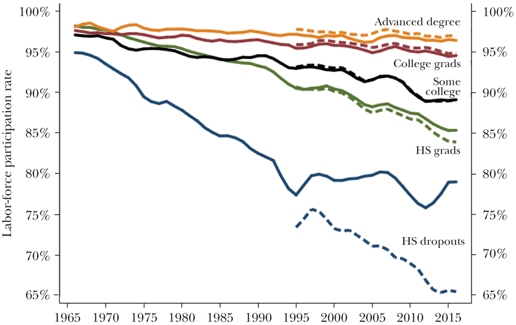
In Figure 2, we plot the 1965–2016 evolution of the labor-force participation rate by education status, using data from the March supplement to the Current Population Survey based on individuals’ reported labor-force statuses in the survey week. The solid series include all prime-age men, while the dashed series exclude foreign-born immigrants. (The Current Population Survey does not record birthplace until 1994.) This exclusion lowers measured participation for high school graduates and dramatically affects the downward trend for those without a high school diploma, reflecting increasing representation of immigrants in this segment of the population combined with their higher participation rates (Borjas 2017). The hourly earnings series presented earlier in Figure 1 are not nearly as sensitive to the exclusion of immigrants.

Figure 2. Labor-Force Participation Rates by Education Status, Males Aged 25–54, 1965–2016.

Source: Authors’ calculations based on the March supplement to the Current Population Survey.

Note: This figure plots the 1965–2016 evolution of the labor-force participation rate by education status, using data from the March supplement to the Current Population Survey based on individuals’ reported labor-force statuses in the survey week. Dotted lines exclude foreign-born (the CPS begins tracking birthplace in 1994). Within each education status, a re-weighting procedure is employed to hold the age distribution constant across each year. See the online Appendix for further details. Graph presents 3-year centered moving averages. “HS” is high school.

As in the case of earnings, we observe a dramatic rise in labor-force participation dispersion across education levels. In 1965, the difference in the participation rate between advanced degree holders and high school dropouts was 3.2 percentage points; by 2015, this difference had widened to 17.6 percentage points. Within the US-born population, the difference in the participation rate between advanced degree holders and high school dropouts was a tremendous 31.5 percentage points in 2015. Clearly, most of the secular decline in prime-age male labor-force participation can be attributed to those without a college degree; we focus on this group for the remainder of the paper.

Breaking the full sample up into demographic subgroups by race, age, and education confirms that the same overall pattern of decline in prime-age male labor-force participation holds true within each subgroup (as detailed in online Appendix Figure A4). However, within a given education status, blacks experienced larger declines than whites at all age levels. This is especially true among high school dropouts, where black participation rates tumbled by 30–40 percentage points. We also note some heterogeneity in participation trends by age: while all age groups have withdrawn from the labor force consistently over the sample period, the rate of withdrawal for young workers aged 25–34 relative to older workers increased slightly after the mid-1990s. (This is apart from high school dropouts aged 45–54, who have experienced alarmingly high rates of withdrawal from the labor force.)

Is Nonparticipation Temporary or Permanent?

Does the point-in-time labor-force participation rate reflect brief periods of nonparticipation experienced by a sizable share of the population, or perpetual nonparticipation experienced by a small share of the population? An account of how nonparticipation is distributed in the population provides information about the appropriate theoretical framework for examining change. For example, the canonical neoclassical labor supply framework conceives of the amount of time spent working, given an hourly wage rate, as an optimal tradeoff between income and substitution effects (Deaton and Muellbauer 1980). This framework cannot readily shed light on the decision not to spend any time working, which represents a corner solution. However, if most men who are not participating at a given point in time will participate in the future, then the standard framework remains a useful tool to analyze (changes in) male participation behavior.

Using retrospective reports from the March Current Population Survey, Juhn, Murphy, and Topel (1991, 2002) argued that the rise in male joblessness since the 1960s was almost entirely the result of a growing number of men withdrawing permanently from the workforce. Using contemporaneous reports of participation, Coglianese (2018) recently challenged this contention, showing that retrospective reports result in an undercount of brief nonparticipation spells. We examine this issue by leveraging two longitudinal sources of labor-force participation data. The data come from a US Census Bureau data product that links Survey of Income and Program Participation (SIPP) respondents to their earnings information from the Social Security Administration (SSA).

Using the data from the Survey of Income and Program Participation, we define participation as working at least one week in the given survey month, and report in the top panel of Table 1 nonparticipation to participation (N → P) transition probabilities for currently nonparticipating subgroups of men with high school education or less. We consider two such groups: men who experienced a transition from participation to nonparticipation within the first 12 sample months, and men who began the sample period as nonparticipants. We observe substantial short-run spells of nonparticipation. Among white high school graduates (without college) who experienced a transition to nonparticipation, 51 percent had returned to the labor force after 3 months, and 77 percent had returned to the labor force after 12 months. Among white high school graduates who began the sample period as nonparticipants, 25 percent were in the labor force after 3 months and 49 percent were in the labor force after 12 months. While there are mild education and racial gradients to these estimates, we note striking consistency across demographic groups.

Table 1.

Male Workforce Attachment over the Short and Long Run for Those with High School Education or Less: Evidence from SIPP–SSA Longitudinal Data, 1978–2011

A: Short-run N→P transition probabilities
Group	Race	Education	1 month	3 months	6 months	12 months
Experienced an P→N transition in first 12 panel month	Whites	Dropouts	0.18	0.45	0.63	0.72
		HS grads	0.19	0.51	0.69	0.77
	Blacks	Dropouts	0.16	0.33	0.50	0.59
		HS grads	0.15	0.38	0.57	0.66
Nonparticipant in first panel month	Whites	Dropouts	0.08	0.24	0.38	0.46
		HS grads	0.09	0.25	0.40	0.49
	Blacks	Dropouts	0.05	0.16	0.24	0.30
		HS grads	0.07	0.18	0.29	0.36
B: Long-run N→P transition probabilities
Group	Race	Education	1 year	2 years	5 years	10 years
Experienced an P→N transition in first 15 years observed	Whites	Dropouts	0.42	0.58	0.76	0.83
		HS grads	0.50	0.66	0.83	0.89
	Blacks	Dropouts	0.34	0.50	0.69	0.77
		HS grads	0.40	0.57	0.76	0.83
Non-participant in first year observed	Whites	Dropouts	0.27	0.39	0.54	0.62
		HS grads	0.43	0.54	0.72	0.81
	Blacks	Dropouts	0.29	0.38	0.51	0.57
		HS grads	0.34	0.47	0.63	0.74

Source: Authors’ calculations based on the 1984–2008 Survey of Income and Program Participation (SIPP) panels (top panel) and SIPP panels linked to Social Security Administration (SSA) earnings records (bottom panel).

Note: Sample consists of men with high school education or less with 0–30 years of potential experience and not enrolled in school at the beginning of the SIPP panel window. “Dropouts” are high school dropouts. “HS grads” are high school graduates without college. Panel A reports the share of men who transitioned out of nonparticipation by the given month—1, 3, 6, or 12 months after the initial experience of nonparticipation. Two groups of men are considered: those who experienced a transition from participation to nonparticipation (a “P → N” transition) within the first 12 panel months, and those who were nonparticipants at the start of the panel window. Panel B considers the SSA earnings records of all SIPP panel respondents over the subset of years 1978–2011 when the respondents had between 0 and 30 years of potential experience. It reports the share of men who transitioned out of nonparticipation by the given year—1, 2, 5, or 10 years after the initial experience of nonparticipation. Yearly participation is defined as having total administrative earnings for the year above a minimum threshold. Two groups of men are considered: those who experienced a transition to nonparticipation within the first 15 years of observation, and those who were nonparticipants in the first year of observation. See main text and the online Appendix available with this paper at the journal website for further details.

Using earnings histories from the Social Security Administration, which exist on a consistently coded basis for the years 1978–2011, we are also able to construct nonparticipation to participation transition probabilities over a longer-run horizon. These are shown in the second panel of Table 1. Following Coglianese (2018), we define yearly participation as a situation in which total administrative earnings for the year exceed the threshold of one-half of the federal minimum wage times 40 hours per week times 13 weeks. We construct two similar groups of nonparticipants: men who experienced a transition to yearly nonparticipation within the first 15 years observed, and men who were nonparticipants in the first year observed. (Because the definition of participation differs between these short- and long-run analyses, the twelve-month probabilities reported in the top panel of Table 1 differ from the one-year probabilities reported in the bottom panel.) Among white high school graduates who experienced a transition to full-year nonparticipation, 66 percent had achieved annual participation two years later, and 83 percent had achieved annual participation five years later. Among white high school graduates who entered the sample as full-year nonparticipants, 54 percent achieved annual participation after two years, and 76 percent achieved annual participation after five years.

These findings indicate substantial churn into and out of the labor force at long-run as well as short-run frequencies.

How Do Jobless Men Survive?

Another important aspect of labor market nonparticipation is an account of how nonparticipating men obtain resources. Table 2 records annual household income statistics for prime-age non-college-educated men with low labor-force attachment. (We define low labor-force attachment as no more than 13 weeks of employment during the reference year.) The March supplement to the Current Population Survey does not fully distinguish among relevant sources of income until 1992; thus, we consider all years from 1992 to 2017. For each education status, the top panel reports average levels of annual income, rounded to the nearest hundred dollars and broken down by income source. This illustrates how much income the average man has access to and where it comes from. The bottom panel records the frequency with which each source of income accounts for the largest share of total household income, thereby illustrating heterogeneity in income receipt.

Table 2.

Household Income Characteristics of Men with Low Labor-Force Attachment by Race, Education, and Age, 1992–2017

	Whites			Blacks
A: High School Dropouts	25–34	35–44	45–54	25–34	35–44	45–54
Average Annual Income ($)
Own earnings	900	1,100	500	500	400	300
Total unearned income	35,000	28,300	28,400	29,200	28,300	23,500
Own disability-related benefits	3,300	5,700	7,600	2,400	4,200	5,400
Own other unearned income	900	1,100	1,500	400	700	900
Cohabitants’ total earnings	21,800	13,100	12,500	18,600	15,800	10,100
Cohabitants’ total unearned income	8,000	7,400	6,100	6,600	6,800	6,300
Household food stamps income	1,000	1,000	700	1,200	800	800
Maximal Source of Income (%)
Own earnings	3	2	2	2	2	1
Own disability-related benefits	12	23	31	10	18	27
Earnings OR unearned income from:
Parents	30	21	11	38	22	16
Spouse	15	20	20	5	12	12
Other HH members	25	20	21	31	31	26
HH food stamps income	4	3	3	4	3	4
Other source or tie	5	6	7	4	5	6
None (living on < $4 per day)	6	5	5	6	7	8
	Whites			Blacks
B: High School Graduates (no college)	25–34	35–44	45–54	25–34	35–44	45–54
Average Annual Income ($)
Own earnings	1,300	1,300	1,300	600	700	600
Total unearned income	43,000	35,900	36,200	36,800	29,200	27,800
Own disability-related benefits	3,100	5,300	7,200	2,400	3,600	5,300
Own other unearned income	1,600	2,100	3,600	800	1,300	2,200
Cohabitants’ total earnings	30,200	19,900	18,000	26,100	17,000	14,100
Cohabitants’ total unearned income	7,400	7,900	6,900	6,600	6,500	5,500
Household food stamps income	700	700	500	900	800	700
Maximal Source of Income (%)
Own earnings	3	3	2	2	2	2
Own disability-related benefits	9	18	25	7	14	24
Earnings OR unearned income from:
Parents	35	21	12	41	23	11
Spouse	14	22	24	7	17	19
Other HH members	25	19	19	29	25	23
HH food stamps income	3	3	2	2	3	3
Other source or tie	6	7	10	5	6	8
None (living on < $4 per day)	5	7	6	7	10	10

Source: Authors’ calculations based on the March Supplement to the Current Population Survey.

Note: “HH” is household. Sample consist of all households in which at least one prime-age, non-college-educated man with low labor-force attachment resided. Low-labor force attachment is defined as no more than 13 weeks of employment in the reference year. Households with imputed sources of income are excluded. Disability-related benefits are not fully identifiable until 1988; food stamps benefits are not identifiable until 1992; as a result, we consider the years 1992–2017. The top subpanels record average levels of the man’s household’s yearly income in 2017 dollars, rounded to the nearest hundred and broken down by income source. The bottom subpanels record the frequency with which each source of earnings accounts for the largest share of total household income. Extremely poor households, which subsist on less than $4 per day (with a square-root equivalence scale to adjust for household size), are classified as having no maximal source of income. See main text and the online Appendix available with this paper at the journal website for additional information on data processing and some additional tabulations.

Low-participating men earn very little income: average earnings across all demographic groups are at or below $1,300—an extremely low amount to live on for an entire year (top panels of parts A and B of Table 2). Accordingly, only 2–3 percent of the time does the man’s own earnings account for the largest share of total household income (bottom panels). Among 45–54 year old men, own-disability-related benefits are relatively important, amounting to around $7,300 for whites and $5,300 for blacks. Own disability benefits constitute the largest share of total household income in 25–30 percent of these cases. While this number is not small, it still represents a distinct minority; and for younger groups, own disability benefits are relatively unimportant. Across all demographic groups, income from other household members appears to be the dominant income source. This is especially true among 25–34 year-old men, where cohabitants’ income accounts for 82–86 percent of total household income on average, and some source of cohabitants’ income accounts for the largest share of household income 70–75 percent of the time. Even among 45–54 year-old men, some source of cohabitants’ income accounts for the largest share of household income in the majority of cases.

In tabulations not shown here, we found that around 40 percent of white high school dropouts, 30 percent of white high school graduates, 53 percent of black high school dropouts, and 44 percent of black high school graduates lived in households with total income below the federal poverty line. Much smaller shares, however—5 to 7 percent of whites and 7 to 10 percent of blacks—lived in extreme poverty (last rows of parts A and B of Table 2). We define extreme poverty as a situation in which household members subsist on less than $4 per day at 2017 prices. (This figure is chosen by implementing a square-root equivalence scale to adjust for household size. For example, the extreme poverty threshold for a four-person household is $4 per day times 365 days times the square root of 4 = $2,920.) Even smaller shares of men—around 3 percent across all groups—lived above the extreme poverty line but depended primarily on food stamps assistance (last rows of parts A and B of Table 2). Thus, while living standards may not be high for these men, the income of other household members plays an effective role in keeping most of them out of extreme poverty.

It is important to reiterate that the above numbers are based on survey data. There is ample reason to believe that the reported earned income figures are underestimates, because episodic sources of income tend to be underreported (Mathiowetz, Brown, and Bound 2002) or even unreported (Edin and Lein 1997; Meyer and Sullivan 2003, in this journal 2012; Bollinger, Hirsch, Hokayem, and Ziliak forthcoming). Recent work using administrative data has demonstrated that survey data understates the incomes of low-income men and overstates the incidence of extreme poverty (Meyer and Mittag 2015; Meyer, Wu, Mooers, and Medalia 2018). However, this work tends to confirm the notion that men with a weak attachment to the workforce largely persist on the incomes of other household members.

Explaining the Decline

Less-educated men have experienced downward trends in wages, employment, and participation since the early 1970s. Therefore, in attempting to explain the latter trends, a reasonable starting point is to ask if changes in the returns to labor market activity can account for the observed decline in labor market activity.

This interpretation of the data gained currency with the work of Juhn, Murphy, and Topel (1991, 2002; see also Juhn 1992). Focusing on the period of the late 1960s through the late 1980s, these authors estimated labor supply curves from repeated cross-sectional and cross-regional data. In both cases, for less-skilled men, they found strong associations between declines in wages and declines in labor market activity, implying an uncompensated labor supply elasticity of around 0.4 for the lowest skilled group.⁸ They interpreted their findings as reflecting labor demand shifts against a stable and upward-sloping supply curve.

We are uncomfortable with this interpretation for two reasons. First, it belies the conventional wisdom that the (uncompensated) labor supply curve for men is inelastic. This conventional wisdom comes from the fact that tremendous wage increases in the United States, Canada, the United Kingdom, and Germany between 1900 and 1970 have all been associated with small declines in the labor-force participation of prime-age men (for international evidence, see Pencavel 1986; for US evidence, see Ruggles 2015). This notion makes economic sense: if leisure is a superior good, we would expect leisure’s share in total household consumption to rise as wages rise. Second, although wages and participation for less-educated men trended downward in tandem throughout the 1970s and 1980s, participation continued to decline after 1995, when wages were comparatively stable (recall Figure 1).

More recent work has also attributed secular decline in less-educated male wages and employment to declining labor demand (Autor 2011; Moffitt 2012; Council of Economic Advisors 2016). For example, Abraham and Kearney (2018) write: “Our review of the evidence leads us to conclude that labor demand factors are the primary drivers of the secular decline in employment over the 1999 to 2016 period.” The growth of support for this connection has come from recent studies of local labor demand shocks. As mentioned earlier, Autor, Dorn, and Hanson (2013) found that commuting zones with rising exposure to manufactured imports from China saw substantive declines in manufacturing employment and wages. Similarly, Charles, Hurst, and Schwartz (2018) estimated that a 10 percent decline in manufacturing employment since 2000 led to an 18 percent decline in wages, a 7.9 percent decline in hours worked, and a 4.6 percentage point decline in employment of less-educated men. These estimates imply an uncompensated labor supply elasticity of above 0.4.

It is important to reconcile such estimates with the conventional wisdom of a small, or zero, uncompensated elasticity of labor supply. One possible reconciliation recognizes that the labor demand shocks in our period of study not only involve wage cuts, but also job losses, including mass layoffs or the closing of establishments. Displaced male workers take some time to return to the workforce (Jacobson, LaLonde, and Sullivan 1993; Autor, Dorn, Hanson, and Song 2014), in part because current local job losses are often associated with subsequent local job losses. For example, Dix-Carneiro and Kovak (2017) found that initial shocks (albeit in Brazil, not the United States) played out over an extended period partly because of the slow adjustment of capital to the initial shocks. In general, several researchers have documented the slowness of local economies to recover from economic shocks (Bartik 1991; Yagan 2017; Austin, Glaeser, and Summers 2018).

After losing work, individuals may not easily transition into new jobs. For instance, Foote and Ryan (2015) showed that medium-skill displaced male workers tend to face few attractive alternatives within their skill class and sector. Jaimovich and Siu (2018) captured this phenomenon in the context of a search model, in which those losing their jobs in declining sectors of the economy must consider whether to search for new work in the declining sector or invest in new skills. Such a framework can capture business cycle patterns but also secular shifts of the Beveridge curve. A parallel literature has illustrated a reluctance of workers to migrate to better labor markets (Kennan and Walker 2011; Dao, Furceri, and Loungani 2017; Zabek 2018), underscoring the potential importance of migration as well as search frictions.

These dimensions of individual and local labor market adjustment following shocks strike us as key factors underlying the strong secular relationship between wages and participation seen in the 1970s, 1980s, and since 2002. Such adjustment frictions are also consistent with the fact that many spells of nonparticipation are not permanent (recall Table 1)—though it may take some time, most displaced individuals do return to the workforce. A labor supply framework that takes these factors seriously may help resolve the apparent inconsistency between the male labor supply behavior revealed by the historical record and that of the more recent period.

The Expansion of Disability Insurance

A parallel explanation for the large increase in less-educated male joblessness despite a comparatively small decrease in the wages of this group rests on factors operating outside of the labor market. An oft-examined factor is the dramatic increase in the availability and generosity of income maintenance programs targeted at people with disabilities. The largest such program is the Social Security Disability Insurance program (DI), of which we provide a brief history in the online Appendix. The DI rolls expanded considerably between the 1960s and early 1990s and have grown more slowly since (for discussion in this journal, see Liebman 2015; online Appendix Figure A5 graphs trends in the population share of men receiving DI benefits by age group).

To assess the extent to which Disability Insurance expansions have impacted the male labor-force participation rate, Bound (1989) proposed the “rejected-applicant” method, which involves comparing participation behavior of those receiving DI benefits to those who applied for benefits but failed to pass the medical screening necessary to be granted benefits. In a sophisticated application of this method, Maestas, Mullen, and Strand (2013) used random variation in stringency across DI case examiners to estimate that prime-age men on the margin short of DI receipt have a labor-force participation rate of 40 percentage points higher than marginal beneficiaries.

Two issues arise when using this estimate to draw broader inferences about how the Social Security Disability Insurance program has impacted prime-age male labor-force participation. First, if the marginal beneficiary is healthier than the average beneficiary, then the marginal beneficiary’s work propensity may be more sensitive to benefit receipt than that of the average beneficiary. Second, estimates based on the rejected-applicant method are conditional on having applied for benefits. Since nonparticipation is necessary for eligibility, application for DI benefits itself may reduce participation. It may also affect rejected applicants’ subsequent participation behavior (Bound 1989, 1991; Parsons 1991): rejected applicants may reapply, time spent out of work may affect rejected applicants’ job prospects, and the act of applying may permanently affect individuals’ identities.

Bound, Lindner, and Waidmann (2014) attempted to circumvent these issues by arguing that the participation rate of individuals who report having a health-related work limitation but who never applied for Disability Insurance benefits should be a conservative upper bound on the participation rate of both rejected and accepted applicants. Using SIPP–SSA data, they reported an employment rate differential between prime-age men with work limitations who never applied for DI benefits and those who were awarded benefits of roughly 50 percentage points. The reported employment differential between rejected applicants and those awarded benefits was roughly 30 percentage points.

Pulling these considerations together, let us conservatively assume that the disincentive for labor-force participation induced by applying for disability benefits outweighs the fact that the marginal beneficiary may be healthier than the average beneficiary. Under this assumption, Maestas, Mullen, and Strand’s (2013) estimate mentioned above provides a lower bound to the effect of the availability of DI benefits on the labor-force nonparticipation rate of 0.40 times the DI participation rate. Additionally, Bound, Lindner, and Waidmann’s (2014) logic yields an upper bound of 0.50 + 0.30 = 0.80 times the DI participation rate under the assumption that the rejected applicant pool is the same size as the beneficiary pool (a slight exaggeration relative to what they report).

Table 3 uses data from the March Current Population Survey to compare prime-age male Disability Insurance and labor-force participation rates, by age and education, between 1975–84 and 2008–2017.⁹ (Decadal averages are used to reduce sampling error.) The last row of the table implements the bounding exercise just described, reporting a conservative upper bound estimate of the contribution of increased DI program participation to the concomitant rise in nonparticipation. Increased DI participation explains virtually none of the rise in nonparticipation among high school dropouts and little of the rise in nonparticipation among high school graduates (without college) below age 45. On the other hand, it could explain up to 25 percent of the rise in nonparticipation among 45–54 year-old high school graduates (without college). In tabulations not shown, we found similar results for the “some college” group.

Table 3.

Assessing the Effect of Greater Receipt of Social Security Disability Insurance (SSDI) on the Secular Decline in Male Labor-Force Participation

		Dropouts			HS graduates
		25–34	35–44	45–54	25–34	35–44	45–54
SSDI participation rate	1975–84	0.030	0.046	0.076	0.009	0.014	0.027
	2008–17	0.022	0.039	0.088	0.022	0.030	0.059
	Change	−0.008	−0.007	0.012	0.013	0.016	0.032
Labor-force nonparticipation rate	1975–84	0.102	0.106	0.153	0.036	0.034	0.070
	2008–17	0.182	0.175	0.304	0.120	0.122	0.171
	Change	0.080	0.069	0.151	0.084	0.088	0.101
SSDI change/OLF changea		−0.100	−0.101	0.079	0.155	0.182	0.317
Conservative upper-bound contribution of SSDI growth to nonparticipation growth
		−4%	−4%	6%	12%	15%	25%

Source: March Supplement to the Current Population Survey.

Note: “Dropouts” are high school dropouts. “HS grads” are high school graduates without college. Decadal averages are used to reduce sampling error. (Highly) conservative upper bounds equal 0.4 times the ratio of SSDI growth to nonparticipation growth when SSDI growth is negative, and 0.8 times the ratio of SSDI growth to nonparticipation growth when SSDI growth is positive. See main text for a discussion of these upper-bound multipliers.

^aOLF is “Outside the Labor Force.”

In addition to the roughness of this bounding exercise, we note that the growth in Disability Insurance participation may be endogenous to falling labor demand. Previous work has demonstrated that adverse local labor demand shocks expand the DI rolls (Black, Daniel, and Sanders 2002; Autor and Duggan 2003; Charles, Li, and Stephens 2018). Rising DI participation may thus underlie some of the adjustment behavior noted above: rather than search for new work, displaced workers in relatively poor health may simply apply for DI.

Mass Incarceration

The size of the US prison population rose dramatically between 1970 and 2000, from roughly 0.1 percent to 0.5 percent of the total resident population (Raphael and Stoll 2013). We have been studying the civilian, noninstitutionalized male population in this paper—so those incarcerated are excluded. However, as incarceration rates have grown, so has the previously incarcerated share of the currently noninstitutionalized population. Bucknor and Barber (2016) estimated that in 2014, between 6.0 and 7.7 percent of all prime-age men had previously been incarcerated. For black men, the rates were between 19.4 and 21.9 percent; for high school dropout men, the rates were between 26.6 and 30.1 percent. Bucknor and Barber do not report cross-tabulations by education and race, but their figures suggest that potentially a substantial fraction of black male dropouts have prior prison records.

Survey data show that men with criminal records are less likely to be employed than observationally similar individuals without records. Employers report a reluctance to hire men with criminal convictions, while audit studies have found that those with criminal records are less likely to be called back for interviews (Holzer, Raphael, and Stoll 2006a, b; Pager 2003, 2007; Pager, Bonikowski, and Western 2009). The most credible estimates of the effect of prior incarceration on employment leverage random assignment of defendants to courtrooms, judges, and prosecutors. Taking this design to data from Harris Country, Texas, Mueller-Smith (2015) found that each additional year behind bars reduced post-release employment propensity by 3.6 percentage points. For felony defendants with stable pre-charge earnings, incarceration for one or more years reduced employment propensity by much larger amounts. Moreover, Mueller-Smith found prior incarceration to increase subsequent criminal activity. Harding, Morenoff, Nguyen, and Bushway (2018) recently found comparable results using data from Michigan.

These estimates strongly support the notion that incarcerating men is likely to have significant effects on their future labor market outcomes (see also Raphael 2014). That said, there is no straightforward way to make inferences from such estimates about the impact of mass incarceration on noninstitutionalized male labor-force participation. First, the estimates vary considerably across different subpopulations. Second, the statistical design delivers causal effects for the marginal, not the average, man incarcerated. Third, the estimates do not capture spillover effects of mass incarceration on local labor markets and communities.¹⁰ Thus, while we do not feel comfortable using available information to estimate even crudely the effect of mass incarceration on the decline in male labor-force participation since the early 1990s, it seems likely that such effects exist and could be of sizable magnitude, especially among populations who have experienced particularly large exposure to prison (high school dropouts and blacks without any college education). We flag this as an important area for further research.

Feedback from the Marriage Market to Male Labor Supply

The above discussions frame a puzzle. On its own, falling labor demand does not sufficiently explain the secular decline in less-educated male labor-force participation—at least, not without allowing for substantial adjustment frictions in the long run as well as the short run. Rising access to Disability Insurance is at most a partial explanation for the 45–54 year-old group and matters quite little for younger men and for high school dropouts. Rising exposure to prison may be a significant factor for dropouts and for blacks without college education, but labor-force participation for these groups began declining decades before prison populations skyrocketed. Certainly no single explanation can sufficiently explain the decline, and even in combination, the explanations appear insufficient.

We suspect that there is another factor at play. We will argue that the prospect of forming and providing for a new family constitutes an important male labor supply incentive; and thus, that developments within the marriage market can influence male labor-force participation. A decline in the formation of stable families produces a situation in which fewer men are actively involved in family provision or can expect to be involved in the future. This removes a labor supply incentive; and the possibility of drawing support from one’s existing family, as shown earlier in Table 2, creates a feasible labor-force exit.

The Retreat from Marriage and Onset of Parental Cohabitation

American family structure has undergone dramatic change since the 1960s, featuring a reduction in the incidence of stable two-parent households that has been concentrated in the non-college-educated population (Cherlin 2014; in this journal, Lundberg, Pollak, and Stearns 2016). We summarize these changes in Table 4. Across all demographic groups without college education, the share of men currently married fell dramatically between 1970 and 2015. Currently-marrieds now make up a distinct minority of the black population without college degree. As of 2015, only white high school graduates above age 35 were married a majority of the time, but even these groups experienced a 30-percentage-point drop in currently-married rates since 1970.¹¹ Similar changes have occurred for the some-college population.

Table 4.

Males Living in Selected Family Arrangements by Race, Education and Age, 1970–2015 (shares)

			Currently married				Living with parent
Race	Education	Age	1970	1985	2000	2015	1970	1985	2000	2015
Whites	Dropouts	25–34	0.81	0.61	0.48	0.37	0.12	0.18	0.22	0.28
		35–44	0.86	0.75	0.59	0.51	0.06	0.09	0.14	0.17
		45–54	0.86	0.79	0.66	0.49	0.04	0.05	0.06	0.12
	HS grads	25–34	0.83	0.63	0.53	0.38	0.10	0.14	0.16	0.25
		35–44	0.90	0.79	0.65	0.58	0.04	0.05	0.10	0.13
		45–54	0.89	0.84	0.74	0.61	0.03	0.03	0.05	0.09
Blacks	Dropouts	25–34	0.65	0.31	0.23	0.14	0.17	0.36	0.40	0.47
		35–44	0.66	0.50	0.32	0.27	0.09	0.16	0.25	0.29
		45–54	0.70	0.58	0.44	0.31	0.02	0.07	0.13	0.20
	HS grads	25–34	0.70	0.42	0.32	0.17	0.13	0.26	0.31	0.41
		35–44	0.70	0.58	0.45	0.38	0.08	0.10	0.18	0.22
		45–54	0.75	0.67	0.53	0.46	0.06	0.06	0.11	0.12

Source: Authors’ calculations based on the March Supplement to the Current Population Survey.

Note: “Dropouts” are high school dropouts. “HS grads” are high school graduates without college. Statistics were calculated in 5-year windows around the specified years: thus 1970 refers to 1968–72; 1985 refers to 1983–87; 2000 refers to 1998–2002; 2015 refers to 2013–17.

Over the same period, the share of men living with at least one parent has risen in equally dramatic fashion. While parental co-residence was a rare event in 1970, by 2015 over one-quarter of whites and 40 percent of blacks aged 25–34 lived with a parent. Older groups experienced a smaller but still substantial rise in parental co-residence, especially considering the extremely low base rates. For example, white high school graduates aged 35–44 experienced a greater-than-threefold increase in the rate of parental co-residence, from 4 percent in 1970 to 13 percent in 2015. In tabulations not shown, we documented similar increases (though starting from higher base rates) in the shares of men cohabiting with parents or other adult relatives.

In this journal, Stevenson and Wolfers (2007) emphasized the contribution of a variety of important developments to the secular decline in marriage, including greater access to contraception, liberalization of family law, changes in home production technology which have reduced gains from task specialization within the household, and changes to how prospective partners match (for example, the rise of online dating). Falling stigmatism of out-of-wedlock childbearing and single motherhood are also likely relevant (Akerlof, Yellen, and Katz 1996).

Others have argued that male earning potential is central to stable marriage formation. Becker (1981) popularized the “specialization-and-exchange” theory of marriage, which predicts that gains from marriage are an increasing function of the gender wage gap. Other work has suggested the influence of “male breadwinner norms”: even after accounting for specialization incentives, the marriage rate appears to decline when a local labor market shock makes men less likely to out-earn women (Bertrand, Kamenica, and Pan 2015). A different paradigm contends that marriage occurs when the level of resources exceeds a standard associated with successful family pursuits (Easterlin 1966, 1987). Ruggles (2015) argued for the importance of declining less-educated male earnings prospects relative to those of their fathers. A variant marriage threshold is the typical living standard within a peer reference group (Gibson-Davis, Edin, and McLanahan 2005; Watson and McLanahan 2011; Ishizuka 2018). In this view, rising income inequality harms the marriage prospects of below-median individuals.

Marriage as a Social Institution for Male Employment

Previous work has associated marriage with a decline in irresponsible male behavior (Akerlof 1998), such as crime (Edlund, Li, Yi, and Zhang 2013) and excessive drug and alcohol use (Duncan, Wilkerson, and England 2006). In the words of Lundberg, Pollak, and Stearns (in this journal, 2016): “If social and economic changes have reduced the value of marriage to noncollege graduates, these changes may also be responsible for a further causal … effect on men’s behavior.”

Male participation in the labor force may also be a socially responsible activity that, like the avoidance of pathological behaviors, is intertwined with stable marriage. To the extent that the gains from marriage depend on male earnings, married men face an additional incentive to find and maintain a job. Indeed, the securing of gainful employment may even be stipulated by men’s (explicit or implicit) marital contracts with their wives. This mechanism has dynamic implications: with the expectation that they will one day marry and provide for a family, single men are incentivized to invest in their future productivity by working today. Doing so also improves their positions in the marriage market, raising their probabilities of matching with high-quality spouses. As marriage rates and attendant marital expectations decrease, so do these labor supply incentives.

We offer an informal assessment of this marriage market mechanism of labor supply in Table 5. We divide the population of interest into three mutually exclusive statuses: men living with at least one parent, unmarried men not living with a parent, and married men not living with a parent. We compute the decline in observed labor-force participation attributable to changes in population shares between these statuses versus changes in labor-force participation rates within each status during the period from 1970–2015. Our proposed mechanism emphasizes the contribution of shifts between statuses (as married men work more than unmarried men and marriage rates have declined), and declining labor-force participation within unmarried statuses (as expectations of stable family formation have declined). The latter process should be especially relevant for younger groups, where future marital expectations have plausibly changed the most.

Table 5.

Family Structure Decompositions of Changes in the Male Labor-Force Participation Rate by Race, Education, and Age between 1970 and 2015 (percentage point changes, except last column )

					Change within
Race	Education	Age	Total change in labor-force participation rate	Change between	Unmarried with parent	Unmarried without parent	Married	Within married contribution to total change
All Men	Dropouts	25–34	−13.5	−4.7	−3.9	−1.4	−3.5	26%
		35–44	−11.0	−3.7	−2.1	−1.8	−3.5	32%
		45–54	−21.0	−5.5	−2.4	−4.7	−8.4	40%
	HS grads	25–34	−11.2	−3.5	−3.6	−1.3	−2.8	25%
		35–44	−11.0	−3.3	−2.2	−1.7	−3.9	35%
		45–54	−14.8	−3.6	−1.7	−3.8	−5.7	39%
Whites	Dropouts	25–34	−21.2	−6.3	−5.3	−3.7	−6.0	28%
		35–44	−23.3	−5.8	−3.5	−4.5	−9.5	41%
		45–54	−33.1	−6.5	−3.1	−8.6	−14.9	45%
	HS grads	25–34	−10.0	−2.8	−3.1	−1.5	−2.7	27%
		35–44	−10.8	−2.9	−2.4	−1.6	−3.9	36%
		45–54	−13.6	−3.2	−1.6	−3.5	−5.3	39%
Blacks	Dropouts	25–34	−31.6	−11.8	−9.9	−6.2	−3.6	11%
		35–44	−27.5	−8.1	−8.1	−6.5	−4.8	17%
		45–54	−35.5	−10.0	−4.4	−11.3	−9.8	28%
	HS grads	25–34	−18.8	−5.3	−7.0	−2.5	−4.0	21%
		35–44	−15.2	−4.2	−2.8	−3.4	−4.8	32%
		45–54	−20.5	−4.8	−2.2	−7.5	−5.9	29%

Source: Authors’ calculations based on the March Supplement to the Current Population Survey.

Note: “Dropouts” are high school dropouts. “HS grads” are high school graduates without college. See online Appendix for detail on how the within/between decomposition was executed. LFP rates were measured in 5-year windows around the beginning and endpoints: thus 1970 refers to 1968–72; 2015 refers to 2013–2017.

As reported in the last column of Table 5, the decline in labor-force participation among those currently married accounts for a minority of the total observed decline in all demographic groups. This is especially true among blacks: the within-married component accounts for less than one-third of the total decline across all black subgroups. We also observe the predicted age gradient: for groups of men aged 25–34, the within-married component accounts for only about one-quarter of the total change, meaning three-quarters came from the unmarried groups and change in status among the groups. Moreover, the 25–34 age groups have experienced almost as large a decline in labor-force participation as the older groups.

This mechanism offers an interpretation of the puzzle of the recent and disproportionate decline in labor-force participation among young males, identified by Aguiar, Bils, Charles, and Hurst (2017). We repeated the above decomposition for the population of men with 0–10 years of potential experience and not enrolled in school, considering changes from 1997–2015. For this group, observed declines in labor-force participation are largely explained by the between-status component and the within-living-with-parents component (as shown in online Appendix Table A4). Today’s less-educated labor market entrants face increasingly small probabilities of forming their own stable families. Thus, while Aguiar et al. (2017) attribute their disproportionate withdrawal from the labor force to the rising value of leisure (stemming from innovations in video gaming technology), we suggest that a marriage-market-based fall in the value of work could be an alternative explanation.

Implications for the Relationship between Labor Demand and Labor Supply

The marriage market mechanism we propose adds complexity to the relationship between male labor demand and labor supply. To the extent that male earning potential positively influences marriage, a decline in male labor demand results in fewer males forming and heading their own stable families. Thus, a male labor demand shock produces—through the marriage market—an indirect effect on male labor supply incentives and resultant labor-force participation.

The recent findings of Autor, Dorn, and Hanson (2018) indicate that this indirect channel may be important. These authors found that rising local exposure to import competition from China led to local declines in the marriage rate and in the share of children living with their fathers. Thus, the large employment effects of local labor demand shocks may embed family-related effects in addition to the other adjustment frictions we have discussed. Family processes may also interact with these other adjustment frictions: for example, by making men more dependent on their adult relatives and less amenable to finding a new occupation or labor market in which to seek employment. In addition, others have argued that mass incarceration has disrupted family formation (for example, Charles and Luoh 2010; Schneider, Harknett, and Stimpson 2018). These relationships further complicate the separate quantification of the various forces driving the decline in male labor-force participation.

Conclusion

During the last 50 years, the earnings of prime-age men in the United States have stagnated and dispersed across the education distribution. At the same time, the labor-force participation rates of men without a college education have steadily declined. While wage and participation trends are often linked for this population, we have argued that this connection cannot solely be the result of an inward labor demand shift across a stable and elastic labor supply curve. The uncompensated labor supply elasticities implied by the twin declines of wages and participation during the 1970s, 1980s, and 2000s appear too large to be plausible. Moreover, labor-force participation continued to decrease in the 1990s while wages were rising. While the increasing availability of disability benefits and the increase in the fraction of the population with prior incarceration exposure may help explain some of the participation decline, we doubt either factor can explain the bulk of the decline.

We have argued that more plausible explanations for the observed patterns involve feedbacks from male labor demand shocks, which often involve substantial job displacement, to worker adjustment frictions and to family structure. Marriage rates, and corresponding male labor supply incentives, have also fallen for reasons other than changing labor demand. Moreover, we have noted interactions between labor demand and disability benefit take-up, and between mass incarceration and family structure. These factors have all converged to reduce the feasibility and desirability of stable employment, leading affected men—who may not often be eligible for disability or other benefits—to participate sporadically in the labor market and depend primarily on family members for income support. In sum, our observations lead us to be skeptical of attempts to attribute the secular decline in male labor-force participation to a series of causal factors acting separately. We prefer an interpretation in which falling labor demand and other interconnected factors have led to substantially lower participation rates among men with less than a college education.

References

- Abraham Katharine G. , and Kearney Melissa S.. 2018. “Explaining the Decline in the U.S. Employment-to-Population Ratio: A Review of the Evidence.” NBER Working Paper 24333. [Google Scholar]
- Acemoglu Daron , and Autor David. 2011. “Skills, Tasks and Technologies: Implications for Employment and Earnings” Chap. 12 in Handbook of Labor Economics, edited by Card David and Ashenfelter Orley, vol. 4, Part B, pp. 1043–1171. Elsevier. [Google Scholar]
- Acemoglu Daron , and Restrepo Pascual. 2018. “Automation and New Tasks: The Implications of the Task Content of Production for Labor Demand.” November, 6 https://economics.mit.edu/files/16338.
- Agan Amanda , and Starr Sonja. 2018. “Ban the Box, Criminal Records, and Racial Discrimination: A Field Experiment.” Quarterly Journal of Economics 133(1): 191–235. [Google Scholar]
- Aguiar Mark, Bils Mark, Charles Kerwin Kofi , and Hurst Erik. 2017. “Leisure Luxuries and the Labor Supply of Young Men.” NBER Working Paper 23552. [Google Scholar]
- Akerlof George A. 1998. “Men Without Children.” Economic Journal 108(447): 287–309. [Google Scholar]
- Akerlof George A., Yellen Janet L. , and Katz Michael L.. 1996. “An Analysis of Out-of-Wedlock Childbearing in the United States.” Quarterly Journal of Economics 111(2): 277–317. [Google Scholar]
- Altonji Joseph G., Bharadwaj Prashant , and Lange Fabian. 2012. “Changes in the Characteristics of American Youth: Implications for Adult Outcomes.” Journal of Labor Economics 30(4): 783–828. [Google Scholar]
- Austin Benjamin, Glaeser Edward , and Summers Lawrence H.. 2018. “Saving the Heartland: Place-Based Policies in 21st Century America” Brookings Papers on Economic Activity, Spring. [Google Scholar]
- Autor David H. 2014. “Skills, Education, and the Rise of Earnings Inequality among the ‘Other 99 Percent.’” Science 344(6186): 843–51. [DOI] [PubMed] [Google Scholar]
- Autor David H. 2011. “The Polarization of Job Opportunities in the U.S. Labor Market: Implications for Employment and Earnings.” Community Investments 23(2): 11–16. [Google Scholar]
- Autor David H., Dorn David , and Hanson Gordon H.. 2013. “The China Syndrome: Local Labor Market Effects of Import Competition in the United States.” American Economic Review 103(6): 2121–68. [Google Scholar]
- Autor David H., Dorn David , and Hanson Gordon. 2018. “When Work Disappears: Manufacturing Decline and the Falling Marriage Market Value of Young Men.” Discussion Paper 11465, IZA Institute of Labor Economics. [Google Scholar]
- Autor David H., Dorn David, Hanson Gordon H. , and Song Jae. 2014. “Trade Adjustment: Worker-Level Evidence.” Quarterly Journal of Economics 129(4): 1799–1860. [Google Scholar]
- Autor David H., Dorn David, Katz Lawrence F., Patterson Christina , and Van Reenen John. 2017. “Concentrating on the Fall of the Labor Share.” American Economic Review 107(5): 180–85. [Google Scholar]
- Autor David H. , and Duggan Mark G.. 2003. “The Rise in the Disability Rolls and the Decline in Unemployment.” Quarterly Journal of Economics 118(1): 157–206. [Google Scholar]
- Autor David H., Katz Lawrence F. , and Kearney Melissa S.. 2006. “The Polarization of the U.S. Labor Market.” American Economic Review 96(2): 189–94. [Google Scholar]
- Autor David H, Katz Lawrence F. , and Kearney Melissa S.. 2008. “Trends in U.S. Wage Inequality: Revising the Revisionists.” Review of Economics and Statistics 90(2): 300–323. [Google Scholar]
- Autor David H., Katz Lawrence F. , and Krueger Alan B.. 1998. “Computing Inequality: Have Computers Changed the Labor Market?” Quarterly Journal of Economics 113(4): 1169–1213. [Google Scholar]
- Autor David H., Levy Frank , and Murnane Richard J.. 2002. “Upstairs, Downstairs: Computers and Skills on Two Floors of a Large Bank.” ILR Review 55(3): 432–47. [Google Scholar]
- Autor David H., Levy Frank , and Murnane Richard J.. 2003. “The Skill Content of Recent Technological Change: An Empirical Exploration.” Quarterly Journal of Economics 118(4): 1279–1333. [Google Scholar]
- Autor David H., Manning Alan , and Smith Christopher L.. 2016. “The Contribution of the Minimum Wage to US Wage Inequality over Three Decades: A Reassessment.” American Economic Journal: Applied Economics 8(1): 58–99. [Google Scholar]
- Bartik Timothy J. 1991. Who Benefits from State and Local Economic Development Policies? Kalamazoo, MI: Upjohn Press. [Google Scholar]
- Becker Gary S. 1981. A Treatise on the Family. Cambridge, MA: Harvard University Press. [Google Scholar]
- Berman Eli, Bound John , and Griliches Zvi. 1994. “Changes in the Demand for Skilled Labor within U.S. Manufacturing: Evidence from the Annual Survey of Manufactures.” Quarterly Journal of Economics 109(2): 367–97. [Google Scholar]
- Bertrand Marianne, Kamenica Emir , and Pan Jessica. 2015. “Gender Identity and Relative Income within Households.” Quarterly Journal of Economics 130(2): 571–614. [Google Scholar]
- Bivens L. Josh. 2007. “The Gains from Trade: How Big and Who Gets Them?” EPI Working Paper 280, Economic Policy Institute. [Google Scholar]
- Black Dan, Daniel Kermit , and Sanders Seth. 2002. “The Impact of Economic Conditions on Participation in Disability Programs: Evidence from the Coal Boom and Bust.” American Economic Review 92(1): 27–50. [DOI] [PubMed] [Google Scholar]
- Blau Francine D. , and Kahn Lawrence M.. 2017. “The Gender Wage Gap: Extent, Trends, and Explanations.” Journal of Economic Literature 55(3): 789–865. [Google Scholar]
- Bollinger Christopher R., Hirsch Barry T., Hokayem Charles M. , and Ziliak James P.. Forthcoming. “Trouble in the Tails? What We Know about Earnings Nonresponse Thirty Years after Lillard, Smith, and Welch.” Journal of Political Economy. [Google Scholar]
- Borjas George J. 2016. We Wanted Workers: Unraveling the Immigration Narrative. New York, NY: W. W. Norton & Company. [Google Scholar]
- Borjas George J. 2017. “The Labor Supply of Undocumented Immigrants.” Labour Economics 46: 1–13. [Google Scholar]
- Bound John. 1989. “The Health and Earnings of Rejected Disability Insurance Applicants.” American Economic Review 79(3): 482–503. [PubMed] [Google Scholar]
- Bound John. 1991. “The Health and Earnings of Rejected Disability Insurance Applicants: Reply.” American Economic Review 81(5): 1427–34. [PubMed] [Google Scholar]
- Bound John , and Johnson George E.. 1992. “Changes in the Structure of Wages During the 1980’s: An Evaluation of Alternative Explanations.” American Economic Review 82(3): 371–92. [PubMed] [Google Scholar]
- Bound John, Lindner Stephan , and Waidmann Timothy. 2014. “Reconciling Findings on the Employment Effect of Disability Insurance.” IZA Journal of Labor Policy 3: Article 11. [DOI] [PMC free article] [PubMed] [Google Scholar]
- Brayne Sarah. 2014. “Surveillance and System Avoidance: Criminal Justice Contact and Institutional Attachment.” American Sociological Review 79(3): 367–91. [Google Scholar]
- Bucknor Cherrie , and Barber Alan. 2016. “The Price We Pay: Economic Costs of Barriers to Employment for Former Prisoners and People Convicted of Felonies.” CEPR Report, Center for Economic and Policy Research. June http://cepr.net/publications/reports/the-price-we-pay-economic-costs-of-barriers-to-employment-for-former-prisoners-and-people-convicted-of-felonies. [Google Scholar]
- Burstein Ariel, Hanson Gordon, Tian Lin , and Vogel Jonathan. 2017. “Tradability and the Labor-Market Impact of Immigration: Theory and Evidence from the U.S.” NBER Working Paper 23330. [Google Scholar]
- Card David. 2009. “Immigration and Inequality.” American Economic Review 99(2): 1–21. [Google Scholar]
- Card David , and Lemieux Thomas. 2001. “Can Falling Supply Explain the Rising Return to College for Younger Men? A Cohort-Based Analysis.” Quarterly Journal of Economics 116(2): 705–46. [Google Scholar]
- Charles Kerwin Kofi, Hurst Erik , and Notowidigdo Matthew J.. 2016. “The Masking of the Decline in Manufacturing Employment by the Housing Bubble.” Journal of Economic Perspectives 30(2): 179–200. [Google Scholar]
- Charles Kerwin Kofi, Hurst Erik , and Schwartz Mariel. 2018. “The Transformation of Manufacturing and the Decline in U.S. Employment.” NBER Macroeconomics Annual vol. 33 http://www.nber.org/chapters/c14081. [Google Scholar]
- Charles Kerwin Kofi, Li Yiming , and Stephens Melvin Jr. 2018. “Disability Benefit Take-Up and Local Labor Market Conditions.” Review of Economics and Statistics 100(3): 416–23. [Google Scholar]
- Charles Kerwin Kofi , and Luoh Ming Ching. 2010. “Male Incarceration, the Marriage Market, and Female Outcomes.” Review of Economics and Statistics 92(3): 614–27. [Google Scholar]
- Cherlin Andrew J. 2014. Labor’s Love Lost: The Rise and Fall of the Working-Class Family in America. New York: Russell Sage Foundation. [Google Scholar]
- Cline William R. 1997. Trade and Income Distribution. Washington, DC: Peterson Institute for International Economics. [Google Scholar]
- Coglianese John. 2018. “The Rise of In-and-Outs: Declining Labor Force Participation of Prime Age Men.” https://scholar.harvard.edu/files/coglianese/files/coglianese_2017_in-and-outs.pdf.
- Copen Casey E., Daniels Kimberly , and Mosher William D.. 2013. “First Premarital Cohabitation in the United States: 2006–2010 National Survey of Family Growth.” National Health Statistics Reports 64: 1–15. [PubMed] [Google Scholar]
- Cortes Patricia. 2008. “The Effect of Low-Skilled Immigration on U.S. Prices: Evidence from CPI Data.” Journal of Political Economy 116(3): 381–422. [Google Scholar]
- Council of Economic Advisers. 2016. “The Long-Term Decline in Prime-Age Male Labor-Force Participation.” June https://obamawhitehouse.archives.gov/sites/default/files/page/files/20160620_cea_primeage_male_lfp.pdf.
- Dao Mai, Furceri Davide , and Loungani Prakash. 2017. “Regional Labor Market Adjustment in the United States: Trend and Cycle.” Review of Economics and Statistics 99(2): 243–57. [Google Scholar]
- Deaton Angus , and Muellbauer John. 1980. Economics and Consumer Behavior. New York, NY: Cambridge University Press. [Google Scholar]
- DiNardo John, Fortin Nicole M. , and Lemieux Thomas. 1996. “Labor Market Institutions and the Distribution of Wages, 1973–1992: A Semiparametric Approach.” Econometrica 64(5): 1001–44. [Google Scholar]
- Dix-Carneiro Rafael , and Kovak Brian K.. 2017. “Trade Liberalization and Regional Dynamics.” American Economic Review 107(10): 2908–46. [Google Scholar]
- Doleac Jennifer L. , and Hansen Benjamin. 2016. “Does ‘Ban the Box’ Help or Hurt Low-Skilled Workers? Statistical Discrimination and Employment Outcomes When Criminal Histories Are Hidden.” NBER Working Paper 22469. [Google Scholar]
- Duncan Greg J., Wilkerson Bessie , and England Paula. 2006. “Cleaning Up Their Act: The Effects of Marriage and Cohabitation on Licit and Illicit Drug Use.” Demography 43(4): 691–710. [DOI] [PubMed] [Google Scholar]
- Easterlin Richard A. 1987. Birth and Fortune, 2nd ed. University of Chicago Press. [Google Scholar]
- Easterlin Richard A. 1966. “On the Relation of Economic Factors to Recent and Projected Fertility Changes.” Demography 3(1): 131–53. [Google Scholar]
- Edin Kathryn J. , and Lein Laura. 1997. Making Ends Meet: How Single Mothers Survive Welfare and Low-Wage Work. New York, NY: Russell Sage Foundation. [Google Scholar]
- Edlund Lena, Li Hongbin, Yi Junjian , and Zhang Junsen. 2013. “Sex Ratios and Crime: Evidence from China.” Review of Economics and Statistics 95(5): 1520–34. [Google Scholar]
- Elsby Michael W. L., Hobijn Bart , and Şahin Ayşegül. 2013. “The Decline of the U.S. Labor Share.” Brookings Papers on Economic Activity no. 2: 1–63. [Google Scholar]
- Feenstra Robert C. , and Hanson Gordon H.. 1996. “Globalization, Outsourcing, and Wage Inequality.” American Economic Review 86(2): 240–45. [Google Scholar]
- Feenstra Robert C. , and Hanson Gordon H.. 1999. “The Impact of Outsourcing and High-Technology Capital on Wages: Estimates for the United States, 1979–1990.” Quarterly Journal of Economics 114(3): 907–40. [Google Scholar]
- Foote Christopher L. , and Ryan Richard W.. 2015. “Labor-Market Polarization over the Business Cycle.” NBER Macroeconomics Annual 29(1): 371–413. [Google Scholar]
- Fortin Nicole M. , and Lemieux Thomas. 1997. “Institutional Changes and Rising Wage Inequality: Is There a Linkage?” Journal of Economic Perspectives 11(2): 75–96. [Google Scholar]
- Fortin Nicole M., Lemieux Thomas , and Lloyd Neil. 2018. “Labor Market Institutions and the Distribution of Wages: The Role of Spillover Effects.” September https://econ2017.sites.olt.ubc.ca/files/2018/12/pdf_paper_thomas-lemieux-spillovers.pdf.
- Freeman Richard B. 1975. “Overinvestment in College Training?” Journal of Human Resources 10(3): 287–311. [Google Scholar]
- Frey Carl Benedikt , and Osborne Michael A.. 2017. “The Future of Employment: How Susceptible Are Jobs to Computerisation?” Technological Forecasting and Social Change 114: 254–80. [Google Scholar]
- Gibson-Davis Christina M., Edin Kathryn , and McLanahan Sara. 2005. “High Hopes but Even Higher Expectations: The Retreat from Marriage among Low-Income Couples.” Journal of Marriage and Family 67(5): 1301–12. [Google Scholar]
- Goffman Alice. 2014. On the Run: Fugitive Life in an American City. University of Chicago Press. [Google Scholar]
- Goldin Claudia , and Katz Lawrence F.. 2008. The Race between Education and Technology. Cambridge, Massachusetts: Belknap Press. [Google Scholar]
- Harding David J., Morenoff Jeffrey D., Nguyen Anh P. , and Bushway Shawn D.. 2018. “Imprisonment and Labor Market Outcomes: Evidence from a Natural Experiment.” American Journal of Sociology 124(1): 49–110. [Google Scholar]
- Hirsch Barry T. 1988. “Trucking Regulation, Unionization, and Labor Earnings: 1973–85.” Journal of Human Resources 23(3): 296–319. [Google Scholar]
- Holzer Harry J. 2010. “Is the Middle of the U.S. Job Market Really Disappearing? A Comment on the ‘Polarization’ Hypothesis.” May 13, Center for American Progress. https://www.americanprogress.org/issues/economy/reports/2010/05/13/7843/is-the-middle-of-the-us-job-market-really-disappearing/. [Google Scholar]
- Holzer Harry J., Raphael Steven , and Stoll Michael A.. 2006a. “How Do Employer Perceptions of Crime and Incarceration Affect the Employment Prospects of Less-Educated Young Black Men?” Chap. 4 in Black Males Left Behind, edited by Mincy Ronald B.. Washington, DC: The Urban Institute Press. [Google Scholar]
- Holzer Harry J., Raphael Steven , and Stoll Michael A.. 2006b. “Perceived Criminality, Criminal Background Checks, and the Racial Hiring Practices of Employers.” Journal of Law and Economics 49(2): 451–80. [Google Scholar]
- Ishizuka Patrick. 2018. “The Economic Foundations of Cohabiting Couples’ Union Transitions.” Demography 55(2): 535–57. [DOI] [PubMed] [Google Scholar]
- Jacobson Louis S., LaLonde Robert J. , and Sullivan Daniel G.. 1993. “Earnings Losses of Displaced Workers.” American Economic Review 83(4): 685–709. [Google Scholar]
- Jaimovich Nir , and Siu Henry E.. 2018. “Job Polarization and Jobless Recoveries.” NBER Working Paper 18334. [Google Scholar]
- Juhn Chinhui. 1992. “Decline of Male Labor Market Participation: The Role of Declining Market Opportunities.” Quarterly Journal of Economics 107(1): 79–121. [Google Scholar]
- Juhn Chinhui, Murphy Kevin M. , and Topel Robert H.. 1991. “Why Has the Natural Rate of Unemployment Increased over Time?” Brookings Papers on Economic Activity, no. 2, pp. 75–142. [Google Scholar]
- Juhn Chinhui, Murphy Kevin M. , and Topel Robert H.. 2002. “Current Unemployment, Historically Contemplated.” Brookings Papers on Economic Activity no. 1, pp. 79–116. [Google Scholar]
- Karabarbounis Loukas , and Neiman Brent. 2014. “The Global Decline of the Labor Share.” Quarterly Journal of Economics 129(1): 61–103. [Google Scholar]
- Katz Lawrence F. 2008. Comment on “Trade and Wages, Reconsidered” by Paul Krugman. Brookings Papers on Economic Activity, no. 1: 143–49. [Google Scholar]
- Katz Lawrence F. , and Murphy Kevin M.. 1992. “Changes in Relative Wages, 1963–1987: Supply and Demand Factors.” Quarterly Journal of Economics 107(1): 35–78. [Google Scholar]
- Kennan John , and Walker James R.. 2011. “The Effect of Expected Income on Individual Migration Decisions.” Econometrica 79(1): 211–51. [Google Scholar]
- Krugman Paul R. 2008. “Trade and Wages, Reconsidered.” Brookings Papers on Economic Activity no. 1, pp. 103–54. [Google Scholar]
- Lee David S. 1999. “Wage Inequality in the United States during the 1980s: Rising Dispersion or Falling Minimum Wage?” Quarterly Journal of Economics 114(3): 977–1023. [Google Scholar]
- Levy Frank , and Murnane Richard J.. 2004. The New Division of Labor: How Computers Are Creating the Next Job Market. Princeton University Press; Russell Sage Foundation. [Google Scholar]
- Liebman Jeffrey B. 2015. “Understanding the Increase in Disability Insurance Benefit Receipt in the United States.” Journal of Economic Perspectives 29(2): 123–50. [DOI] [PubMed] [Google Scholar]
- Lundberg Shelly, Pollak Robert A. , and Stearns Jenna. 2016. “Family Inequality: Diverging Patterns in Marriage, Cohabitation, and Childbearing.” Journal of Economic Perspectives 30(2): 79–102. [DOI] [PMC free article] [PubMed] [Google Scholar]
- Maestas Nicole, Mullen Kathleen J. , and Strand Alexander. 2013. “Does Disability Insurance Receipt Discourage Work? Using Examiner Assignment to Estimate Causal Effects of SSDI Receipt.” American Economic Review 103(5): 1797–1829. [Google Scholar]
- Mathiowetz Nancy A., Brown Charles , and Bound John. 2002. “Measurement Error in Surveys of the Low-Income Population” Chap. in Studies of Welfare Populations: Data Collection and Research Issues. National Academies Press. [Google Scholar]
- Mazzolari Francesca , and Ragusa Giuseppe. 2013. “Spillovers from High-Skill Consumption to Low-Skill Labor Markets.” Review of Economics and Statistics 95(1): 74–86. [Google Scholar]
- Meyer Bruce D. , and Mittag Nikolas. 2015. “Using Linked Survey Data and Administrative Data to Better Measure Income: Implications for Poverty, Program Effectiveness and Holes in the Safety Net.” NBER Working Paper 21676. [Google Scholar]
- Meyer Bruce D. , and Sullivan James X.. 2003. “Measuring the Well-Being of the Poor Using Income and Consumption.” Journal of Human Resources 38(Special Issue on Income Volatility and Implications for Food Assistance Programs): 1180–1220. [Google Scholar]
- Meyer Bruce D. , and Sullivan James X.. 2012. “Identifying the Disadvantaged: Official Poverty, Consumption Poverty, and the New Supplemental Poverty Measure.” Journal of Economic Perspectives 26(3): 111–36. [Google Scholar]
- Meyer Bruce D., Wu Derek, Mooers Victoria , and Medalia Carla. 2018. “The Use and Misuse of Income Data and the Rarity of Extreme Poverty in the United States.” Working paper. [Google Scholar]
- Moffitt Robert A. 2012. “The Reversal of the Employment-Population Ratio in the 2000s: Facts and Explanations.” Brookings Papers on Economic Activity, Fall, pp. 201–64. [Google Scholar]
- Mueller-Smith Michael. 2015. “The Criminal and Labor Market Impacts of Incarceration.” https://sites.lsa.umich.edu/mgms/wp-content/uploads/sites/283/2015/09/incar.pdf.
- Murphy Daniel. 2016. “Welfare Consequences of Asymmetric Growth.” Journal of Economic Behavior & Organization 126(Part A): 1–17. [Google Scholar]
- Murphy Kevin M. , and Welch Finis. 1991. “The Role of International Trade in Wage Differentials” Chap. 2 in Workers and Their Wages Changing Patterns in the United States, edited by Kosters Marvin H.. Washington, DC: AEI Press. [Google Scholar]
- Murphy Kevin M. , and Welch Finis. 1992. “The Structure of Wages.” Quarterly Journal of Economics 107(1): 285–326. [Google Scholar]
- Pager Devah. 2003. “The Mark of a Criminal Record.” American Journal of Sociology 108(5): 937–75. [Google Scholar]
- Pager Devah. 2007. Marked: Race, Crime, and Finding Work in an Era of Mass Incarceration. University of Chicago Press. [Google Scholar]
- Pager Devah, Bonikowski Bart , and Western Bruce. 2009. “Discrimination in a Low-Wage Labor Market: A Field Experiment.” American Sociological Review 74(5): 777–99. [DOI] [PMC free article] [PubMed] [Google Scholar]
- Parsons Donald O. 1991. “The Health and Earnings of Rejected Disability Insurance Applicants: Comment.” American Economic Review 81(5): 1419–26. [Google Scholar]
- Pencavel John. 1986. “Labor Supply of Men: A Survey” Chap. 1 in Handbook of Labor Economics, vo1. 1, edited by Ashenfelter Orely C. and Layard Richard, 3–102. Elsevier. [Google Scholar]
- Peri Giovanni. 2016. “Immigrants, Productivity, and Labor Markets.” Journal of Economic Perspectives 30(4): 3–30. [Google Scholar]
- Peri Giovanni , and Sparber Chad. 2009. “Task Specialization, Immigration, and Wages.” American Economic Journal: Applied Economics 1(3): 135–69. [Google Scholar]
- Raphael Steven. 2014. The New Scarlet Letter? Negotiating the U.S. Labor Market with a Criminal Record. Kalamazoo, MI: W.E. Upjohn Institute. [Google Scholar]
- Raphael Steven , and Stoll Michael A.. 2013. Why Are So Many Americans in Prison? Russell Sage Foundation. [Google Scholar]
- Rose Nancy L. 1987. “Labor Rent Sharing and Regulation: Evidence from the Trucking Industry.” Journal of Political Economy 95(6): 1146–78. [Google Scholar]
- Ruggles Steven. 2015. “Patriarchy, Power and Pay: The Transformation of American Families, 1800–2015.” Demography 52(6): 1797–1823. [DOI] [PMC free article] [PubMed] [Google Scholar]
- Schneider Daniel, Harknett Kristen , and Stimpson Matthew. 2018. “What Explains the Decline in First Marriage in the United States? Evidence from the Panel Study of Income Dynamics, 1969 to 2013.” Journal of Marriage and Family 80(4): 791–811. [Google Scholar]
- Stevenson Betsey , and Wolfers Justin. 2007. “Marriage and Divorce: Changes and Their Driving Forces.” Journal of Economic Perspectives 21(2): 27–52. [Google Scholar]
- Watson Tara , and McLanahan Sara. 2011. “Marriage Meets the Joneses: Relative Income, Identity, and Marital Status.” Journal of Human Resources 46(3): 482–517. [DOI] [PMC free article] [PubMed] [Google Scholar]
- Yagan Danny. 2017. “Employment Hysteresis from the Great Recession.” NBER Working Paper 23844. [Google Scholar]
- Zabek Mike. 2018. “Local Ties in Spatial Equilibrium.” https://mikezabek.com/pdf/LocalTies.pdf.
Associated Data
This section collects any data citations, data availability statements, or supplementary materials included in this article.