Operations Research Methods for Estimating the Population Size of Neuron Types

Abstract

Understanding brain computation requires assembling a complete catalog of its architectural components. Although the brain is organized into several anatomical and functional regions, it is ultimately the neurons in every region that are responsible for cognition and behavior. Thus, classifying neuron types throughout the brain and quantifying the population sizes of distinct classes in different regions is a key subject of research in the neuroscience community. The total number of neurons in the brain has been estimated for multiple species, but the definition and population size of each neuron type are still open questions even in common model organisms: the so called “cell census” problem. We propose a methodology that uses operations research principles to estimate the number of neurons in each type based on available information on their distinguishing properties. Thus, assuming a set of neuron type definitions, we provide a solution to the issue of assessing their relative proportions. Specifically, we present a three-step approach that includes literature search, equation generation, and numerical optimization. Solving computationally the set of equations generated by literature mining yields best estimates or most likely ranges for the number of neurons in each type. While this strategy can be applied towards any neural system, we illustrate its usage on the rodent hippocampus.

1. Introduction

A quantitative description of the brain’s machinery is essential to understand the mechanisms of nervous system functions. The brain encompasses an extraordinary quantity and diversity of cells. The human brain contains nearly 100 billion neurons (Herculano-Houzel 2009) and the rodent brain contains around 100 million neurons (Herculano-Houzel et al. 2011). Neurons can be grouped into many distinct types based on their structural, physiological and molecular features (Bota and Swanson 2007; Shepherd et al. 2019). The composition of balanced proportions of neuron types into elaborate networks enables the brain’s many specific computations. Estimated counts of neuronal types, i.e. a “neuronal census”, would enable more accurate and complete models of brain circuits. Towards this goal, the National Institutes of Health launched the BRAIN Initiative Cell Census Network (BICCN), a consortium of research projects tasked with generating a comprehensive molecular and anatomical cellular “parts list” within a three-dimensional reference mouse whole-brain atlas (Ecker et al. 2017).

Counting the neurons of each type in a region requires establishing the identity of millions of individual neurons. Rapid progress in genetic phenotyping is on the verge of enabling a comprehensive cell-level classification of neurons throughout the mouse cortex (Tasic et al. 2018). However, linking these growing molecular data to anatomical connectivity requires the analysis of the neuronal input and output elements, namely dendritic and axonal arbors. Full morphological characterization of axons and dendrites involves physical or optical tissue sectioning to follow the complex branching structures in the dense three-dimensional space. This is a labor-intensive and error-prone procedure for a human to perform manually, underscoring the need for increasingly automated machine-learning approaches (Peng et al. 2015; Januszewski et al. 2018). Experimentally, the problem is exacerbated by the large disproportion between the total length of an individual axon (hundreds of millimeters) and its branch thickness (tens of nanometers), resulting in a very small ratio (~10⁻⁷) between the volume of a neuronal projection and the territory it spans. This major obstacle will likely keep the acquisition of comprehensive structural data at single-neuron resolution below full-brain scale for many years. Therefore, indirect estimation of neuron type population counts is an important and useful endeavor.

The neuroscience literature contains a great deal of data relevant to the census problem. These include stereological sampling of neuronal densities in specific anatomical areas, morphological characterizations of collections of neurons from the same brain region, slice imaging of neurons stained for a particular molecular marker, and more (Hamilton et al. 2012; White et al. 2019). Each of these data types expresses facts about absolute or relative neuronal population sizes. Integrating such diverse sources of information for a neuronal census poses two primary challenges: formatting all relevant observations in terms of a common neuronal classification scheme; and inferring population sizes from the properly formatted evidence. Solving the first challenge will ultimately require a broad consensus in the neuroscience community on how to define neuron types objectively and reproducibly (Armañanzas and Ascoli 2015). For the purpose of illustration, in this study we tentatively adopt a recent circuit-based classification proposal (Ascoli and Wheeler 2016) for which relatively abundant data are available for parts of the rodent brain such as the hippocampus.

Solving the second challenge entails a workflow for integrating contrasting measurements and interpolating through missing data points. Operations research offers many techniques for leveraging inconsistent and/or incomplete information to achieve an optimal estimate for a set of target parameters. These techniques fall under the broad umbrella of mathematical optimization. Here we describe the use of mathematical optimization to obtain an estimated neuronal census. The neuronal population counts to be estimated are represented as free parameters. Data relating neuron types to their properties (e.g. from literature search or experiment) are formatted as equations in terms of these parameters. These equations are composed into an objective function, which can be optimized by a variety of algorithms. Thus the novelty of this work consists of applying, for the first time, established operations research strategies to the open neuroscience problem of the brain cell census. The present study illustrates the proposed approach with a concrete application to a subregion of the hippocampal formation of the mammalian brain.

2. Methods

In order to describe the operations research aspects of our approach, we first explain how it is possible to derive a system of equations encoding constraints for a neuronal census. In the most general sense, every neuron type is associated with a distinct collection of properties (e.g. morphological, physiological or molecular) through a many-to-many relationship. In other words, no single property uniquely identifies a neuron type, and any property is typically associated with multiple neuron types. However, the full set of properties of a given neuron type is indeed different from that of all other neuron types. Useful constraints consist of measurements, observations or reports on neuronal properties that can link combinations of neuron types to specific numerical values.

Consider for instance a brain region with only two neuron types, A and B, and corresponding counts n_A and n_b. If a stereology experiment determines the total number of neurons in that region to be 1000, this provides a useful constraint (and corresponding equation) by setting the sum of the two target counts to the measured value (n_A + n_B = 1000). Now suppose that only neuron type A expresses a particular protein and an article reports that, out of 20 cells tested in that region, 15 were found to be positive for that protein while 5 were negative. This provides another useful constraint (and a second equation) by indicating a ratio (3:1) between the two target values ($\frac{n_A}{n_B}=3$). In this simple case the number of equations equals the number of unknown counts, yielding a well-constrained system with a single exact solution (n_A = 750, n_B = 250).

In a more general sense, a system of equations is overdetermined if there are more constraints (equations) than parameters and underdetermined if there are fewer constraints than parameters. In the census problem, overdetermined systems may arise from multiple experiments measuring the same variable (e.g. the total number of neurons in a region) and yielding inconsistent results. Unless the equations are trivially redundant, overdetermined systems are inconsistent and thus do not have exact solutions. In this case numerical optimization may find a best estimate that minimizes the discrepancy from all available constraints. Underdetermined systems arise when insufficient constraints are available for one or more of the target unknowns. If none of the constraints are mutually inconsistent, an underdetermined system typically has an infinite number of solutions. In this case numerical optimization may find the range of values defining the possible solutions.

2.1. Classification and analysis framework

As a pilot study, we applied our methodology to estimate the population size of each known neuron type in the hippocampal subregion of the dentate gyrus (DG). This required a neuronal classification scheme for the dentate gyrus. We defined DG cell types based on the knowledge base Hippocampome.org, an online repository containing morphological, molecular, and physiological information on neurons of the rodent hippocampal formation (Wheeler et al. 2015). Hippocampome.org classifies neurons primarily by neurotransmitter released and the presence of axons and dendrites in the distinct subregions and layers of the rodent hippocampus (Figure 1). It also includes molecular biomarker (Hamilton et al. 2017) and electrophysiological properties (Moradi and Ascoli et al. 2019) for each type. Hippocampome.org identifies 18 distinct neuron types in DG: 14 with cell bodies exclusively present in a single layer and 4 with cell bodies distributed across two layers. Thus, the target unknowns or decision variables for this neuronal census consist of the population counts for 22 layer-wise types, which we represent here with parameters x₁, x₂, … x₂₂ (Table 1).

Fig. 1.

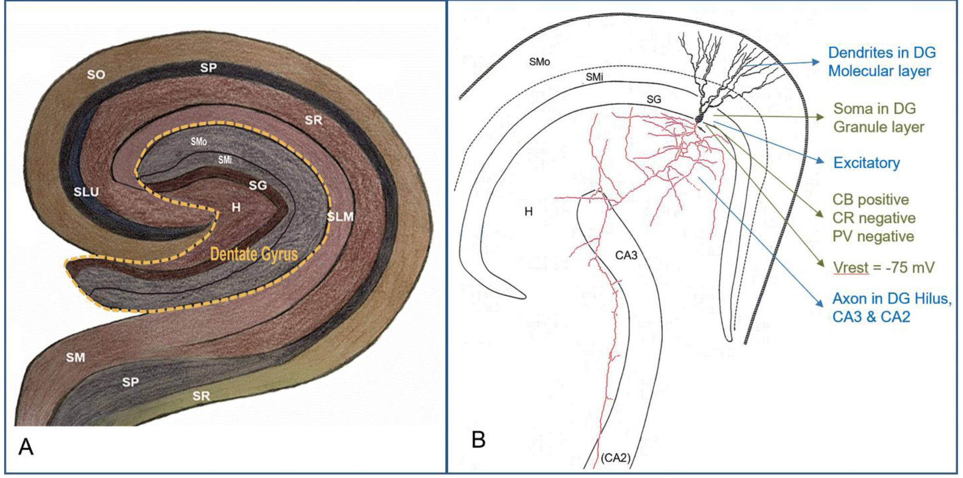
Hippocampome.org neuron type classification. A. Layer organization of the rodent hippocampus, highlighting the dentate gyrus and surrounding regions. B. A dentate gyrus granule cell (cell body and dendrites: black, axon: red) with color-coded properties (neurotransmitter and axonal-dendritic distributions: blue; molecular expression and electrophysiology: green). Label abbreviations: CB: calbindin; CR, calretinin; H, Hilus; PV, parvalbumin; SG, stratum granulosum; SLM, stratum lacunosum-moleculare; SLU, stratum lucidum; SM/SMi/SMo, stratum moleculare (inner/outer); SP, stratum pyramidale; SR, stratum radiatum; Vrest, resting voltage potential.

Table 1.

Layer-specific neuron types (left) and decision variables representing corresponding counts (right). See legend of Fig. 1 for layer abbreviation definitions. For the 4 neuron types with cell bodies distributed across two layers, the naming scheme follows the convention ‘layer: type’.

Neuron type	Decision variable
Granule	x1
Hilar Ectopic Granule	x2
Semilunar Granule	x3
Mossy	x4
Mossy MOLDEN	x5
AIPRIM	x6
Axo-Axonic	x7
Basket	x8
SG: Basket CCK+	x9
SMi: Basket CCK+	x10
H: HICAP	x11
SG: HICAP	x12
H: HIPP	x13
SG: HIPP	x14
HIPROM	x15
MOCAP	x16
MOLAX	x17
SMi: MOPP	x18
SMo: MOPP	x19
Neurogliaform	x20
Outer Molecular Layer	x21
Total Molecular Layer	x22

Our methodology in estimating the neuron type counts consists of three steps: (i) searching for actionable information regarding neuronal counts from the peer reviewed literature, (ii) assembling a set of equations by mapping the extracted information to the chosen neuron type classification scheme, and (iii) numerically optimizing these equations by minimizing an objective function (discrepancy from empirical evidence) to derive type-specific counts (Figure 2).

Fig. 2.

Methodological pipeline to estimate neuron type counts through three sequential phases: literature mining, data processing, and numerical optimization. HCO: Hippocampome.org

2.2. Literature search

Our literature mining protocol began with an analysis of the bibliography of Hippocampome.org v.1.7 (hippocampome.org/php/Help_Bibliography.php). Hippocampome.org lists 496 publications used as evidence for the definition of neuronal types. Each of the dentate gyrus neuron types that are the subject of this study is associated with at least one, but typically several, such publication(s). The full text of each DG publication was evaluated for relevance and selected for further mining if it contained at least one of four kinds of data: stereology-based measurements of cell counts or densities; counts or densities derived from image processing techniques; morphological ratios obtained from studies that reconstructed small samples of neurons for electrophysiological analysis; and inferences based on volumetric estimates and indirect evidence.

Stereology aims to obtain unbiased estimates of cell numbers by inferring population sizes in three dimensions from two-dimensional slice images. A traditional stereological technique is the “optical disector” (Russ and Dehoff 2012), which uses a varying focal plane to obtain many optical “slices” of an intact piece of tissue. A relatively newer method, the optical fractionator, transforms the highly anisotropic tissue into a homogeneous suspension of free-floating nuclei which can then be counted microscopically or by flow cytometry and identified morphologically or immunocytochemically (Herculano-Houzel 2015). In general, stereology requires specific training, equipment, and histological processing, as well as appropriate sampling strategies, careful calibration, and rigorous statistical analysis (Bartheld et al. 2001). Recently, newer image processing techniques for automated object segmentation have enabled cell counting from an entire brain region of interest without need of sampling (Bhanu and Peng 2000; Peng et al. 2013; Attili et al. 2019). Morphological ratios are derived from electrophysiological experiments, such as patch clamp recordings, designed to understand the cell properties in a specific neural system. Unlike stereology, electrophysiological cell sampling is not optimized for counting.

Papers from the Hippocampome.org bibliography containing any of the above information were further mined for any reference cited in the context of the above information; moreover, all references citing the selected papers were also mined if their title explicitly referred to relevant neuron type data. Stereology-based measurements and image processing calculations were considered more reliable than morphological ratios and indirect inferences. This is because stereology and image processing are designed to obtain accurate population counts, while morphological ratios typically come from experiments that use unclear sampling methodologies and inferences are based on uncertain assumptions. Therefore, stereology/image processing constraints were weighted 10:1 against morphological ratios and indirect inference constraints. Rodent scaling rules (Herculano-Houzel et al. 2006) were used to integrate mouse data with most of the available information that is specific to rats.

2.3. Data processing

The sets of neurons described by the authors of the identified articles typically did not directly align with the Hippocampome.org classification scheme. Thus, constraint formation required mapping the literature-defined neuron types (literature types) to Hippocampome.org types. Since each Hippocampome.org type has a unique set of morphological, electrophysiological, and biochemical properties, we translated the description of each literature type into a similarly formalized set of properties, which we then used to match one or more Hippocampome.org types. The literature type could next be assigned the variable(s) x_i associated with the matching type(s). When a literature type had properties matching multiple Hippocampome.org types, the sum of the variables representing the corresponding Hippocampome.org types was used. As an example of an equation generated from an electrophysiological experiment, one of the mined articles (Ceranik et al. 1997) states:

“Neurons from dentate gyrus outer molecular layer were recorded and filled with biocytin for videomicroscopy. 40 neurons were adequately stained. Out of these, 6 neurons were identified as displaced granule cells, 14 neurons had a local axonal arborization that was confined mainly to the OML, 3 projected to the stratum lacunosum moleculare of the CA1 region, and 17 neurons projected to the subiculum via the hippocampal fissure.”

In this description, the author defines four different groups of neurons having somata in the DG outer molecular layer (SMo in Fig. 1 and Table 1 above). Based on the descriptions of their axons, the groups of 14 and 17 neurons were matched to unique Hippocampome.org types MOPP and DG Neurogliaform, respectively. This allowed us to construct the equation $\frac{x_{19}}{x_{20}}= \frac{14}{17}$, where x₁₉ and x₂₀ are the parameters representing the respective outer molecular layer counts of MOPP and Neurogliaform cells. Equations were converted to a percent-error format for optimization ($\frac{17x_{19}}{14x_{20}}-1=\epsilon$), where Ɛ is the error term (residual). The “displaced granule cells” and “3 projecting to the stratum lacunosum moleculare” represented groups with no corresponding Hippocampome.org types, so similar equations could not be constructed for these groups.

2.4. Optimization

Let a vector containing population counts x₁, x₂, … x_n be a “count vector” x. Then, given a set of constraints c₁, c₂, … c_m and corresponding weights w₁, w₂, … w_m, our goal is to find a count vector $\widehat{x}$ that best satisfies the weighted constraints. There are multiple plausible ways to formulate this optimization problem. One approach is to express our constraints as a linear system of equations. This presents a linear least squares problem that can be easily solved with popular methods. Unfortunately constraints are implicitly weighted in this formulation by the magnitudes of the known parameters they contain. The resultant massive and arbitrary weight disparities undesirably bias optimization results. Below we demonstrate this fact and present an alternative formulation that minimizes the weighted percent errors of each constraint.

2.4.1. Linear formulation

To formulate the problem as linear least squares, we need to derive from each constraint c_i a linear equation in x. Our constraint set consists of two kinds of constraints, sums and ratios:

$$x_6+x_{11}+x_{13}+x_{15}=16,801\left(\mathit{\text{sum}}\right)$$

$$\frac{x_{19}}{x_{20}}=\frac{6}{11}\left(\mathit{\text{ratio}}\right)$$

Sum constraints are already linear equations in x. Ratio constraints can be converted into linear equations in x:

$$\frac{x_{19}}{x_{20}}=\frac{6}{11} \to 11x_{19}-6x_{20}=0$$

Thus, all constraints have a corresponding linear equation. This allows us to formulate the matrix equation Ax = b, with A an m × n matrix with rows corresponding to the left-hand-side coefficients for each equation, and b a vector containing the right-hand-side constants or known parameters. The equation has no solution because our linear system is overdetermined and inconsistent, but there exists a best fit $\widehat{\mathit{x}}$ that minimizes the sum of squared errors. We need to place boundary conditions on $\widehat{\mathit{x}}$, since neuron counts cannot be too small or large. We also wish to differentially weight the constraints arising from different source experiments. Now let L_i and U_i be lower and upper bounds for x_i, and let W be an m × m diagonal matrix with weights w₁, w₂, … w_m the diagonal. Then we can define the problem as follows:

$${\epsilon }_i^L\left(\mathit{x}\right)= \sum _{j=1}^n\left(A_{ij}{x}_j\right)-b_i$$

$$\sum _{i=1}^m{w}_i{\left({\epsilon }_i^L\left(\mathit{x}\right)\right)}^2={\Vert {\mathit{W}}^{\frac{1}{2}}\left(\mathit{A}\mathit{x}-\mathit{b}\right)\Vert }^2$$

$$\widehat{\mathit{x}}=ar{g}_{x}min \Vert {\mathit{W}}^{\frac{1}{2}}\left(\mathit{A}\mathit{x}-\mathit{b}\right){\Vert }^2$$

$$\mathit{\text{subject to}}{L}_i\le x_i\le U_{i}for{x}_i\in x$$

This is a constrained, weighted, linear least squares optimization problem. Most numerical programming environments provide off-the-shelf routines that can efficiently solve this type of problem (e.g. scipy.optimize.lsq_linear in Python, bvls in R).

Unfortunately, this formulation has an undesirable property for count estimation. Our constraints contain known parameters of widely varying magnitudes. Consider the error terms ${\epsilon }_a^L\left(\mathit{x}\right)$ and ${\epsilon }_b^L\left(\mathit{x}\right)$ for two of our sum constraints:

$${\epsilon }_a^L\left(\mathit{x}\right)=\left(x_1+x_7+x_8+x_9+x_{12}+x_{14}+x_{16}+x_{17}+x_{21}+x_{22}\right)-1,200,000$$

$${\epsilon }_b^L\left(x\right)=\left(x_6+x_{11}+x_{13}+x_{15}\right)-16,801$$

Now suppose we have a count vector x* such that both constraints a and b are violated by some common factor F. Then ${\epsilon }_a^L\left({\mathit{x}}^{*}\right)$ and ${\epsilon }_b^L\left({\mathit{x}}^{*}\right)$ are:

$${\epsilon }_a^L\left({\mathit{x}}^{*}\right)=1,200,000F-1,200,000=1,200,000\left(F-1\right)$$

$${\epsilon }_b^L\left({\mathit{x}}^{*}\right)=16,801F-16,801=16,801\left(F-1\right)$$

The ratio of the errors is:

$$\frac{{\epsilon }_a^L\left(\mathit{x}\right)}{{\epsilon }_b^L\left(\mathit{x}\right)}=\frac{1,200,000\left(F-1\right)}{16,801\left(F-1\right)}=\frac{1,200,000}{16,801}\approx 71$$

Thus, when constraints c_a and c_b are equally violated in percentage terms, our squared error objective function penalizes the deviation from c_a approximately 71² = 5,041 times more than the deviation from c_b. Thus constraints are implicitly weighted according to the size of the known parameters (constants) they contain. This property is undesirable, since there is no reason to expect the precision of the source measurements to increase with their magnitude. One could eliminate the implicit weighting for sum constraints by normalizing with respect to the measured count. However, no equivalent operation is available for ratio constraints. Therefore, the linear formulation is a poor choice for application to counts estimation.

2.4.2. Percent error formulation

We can avoid the implicit weighting in the linear formulation by directly optimizing the percent errors of each constraint. Let LHS_i (x) and RHS_i be the left and right sides of the measurement form of constraint c_i (all x_i on left, measured constant on right; see ‘Equations’ in supplementary materials). Incorporating weights and boundary constraints, minimization of the squared percent errors gives the optimization problem: i:

$${\epsilon }_i^P\left(\mathit{x}\right)=\frac{LH{S}_i\left(\mathit{x}\right)-RH{S}_i}{RH{S}_i}=\frac{LH{S}_i\left(\mathit{x}\right)}{RH{S}_i}-1$$

$$\widehat{\mathit{x}}=ar{g}_{x}min\sum _{i=1}^m{w}_i{\left({\epsilon }_i^P\left(\mathit{x}\right)\right)}^2$$

$$\mathit{\text{subject to }}{L}_i\le x_i\le U_{i}for{x}_i\in x$$

This formulation does not suffer from the implicit constraint weighting of the linear approach. Equations constructed in this manner have been listed in Table 2.

Table 2.

Representative equations and scientific meaning with original source, type of experimental evidence, and corresponding weights (Wt.).

Equation	Interpretation	Source	Experimental evidence	Wt.
$$\begin{gathered} \frac{x_6}{16801}+ \frac{x_{11}}{16801}+ \frac{x_{13}}{16801}+ \frac{x_{15}}{16801}-1= \\ \epsilon \end{gathered}$$	Count of inhibitory hilar neurons is 16,801	Buckmaster & Jongen-Relo 1999, Table 1	Stereology	10
$$\begin{gathered} \frac{x_1}{1080000}+\frac{x_7}{1080000}+ \frac{x_8}{1080000}+ \\ \frac{x_9}{1080000}+ \frac{x_{12}}{1080000}+ \frac{x_{14}}{1080000}+ \\ \frac{x_{16}}{1080000}+ \frac{x_{17}}{1080000}+ \frac{x_{21}}{1080000}+ \\ \frac{x_{22}}{1080000}-1= \epsilon \end{gathered}$$	Count of granule layer neurons is 1,080,000	Hosseini-Sharifabad and Nyengaard 2007, p209	Stereology	10
$$\begin{gathered} \frac{x_2}{65420}+\frac{x_4}{65420}+ \frac{x_5}{65420}+ \frac{x_6}{65420}+ \\ \frac{x_{11}}{65420}+ \frac{x_{13}}{65420}+ \frac{x_{15}}{65420}-1= \epsilon \end{gathered}$$	Count of all neurons in hilus is 65,420	Grady et al. 2003, Table 1	Stereology	10
$$\begin{gathered} \frac{x_1}{1258848}+\frac{x_2}{1258848}+ \frac{x_3}{1258848}+ \\ \frac{x_4}{1258848}+ \frac{x_5}{1258848}+ \frac{x_6}{1258848}+ \\ \frac{x_7}{1258848}+ \frac{x_8}{1258848}+ \frac{x_9}{1258848}+ \\ \frac{x_{10}}{1258848}+ \frac{x_{11}}{1258848}+ \frac{x_{12}}{1258848}+ \\ \frac{x_{13}}{1258848}+ \frac{x_{14}}{1258848}+ \frac{x_{15}}{1258848}+ \\ \frac{x_{16}}{1258848}+ \frac{x_{17}}{1258848}+ \frac{x_{18}}{1258848}+ \\ \frac{x_{19}}{1258848}+ \frac{x_{20}}{1258848}+ \frac{x_{21}}{1258848}+ \\ \frac{x_{22}}{1258848}-1= \epsilon \end{gathered}$$	Total count of dentate gyrus neurons is 1,258,848	Erö et al. 2018, Supplementary data (Mouse bilateral values, halved and converted to rat)	Image processing	10
$$\begin{gathered} \frac{x_3}{189693}+ \frac{x_{10}}{189693}+ \frac{x_{18}}{189693}+ \frac{x_{19}}{189693}+ \\ \frac{x_{20}}{189693}-1= \epsilon \end{gathered}$$	Count of all neurons in the molecular layer is 189,693	Attili et al. 2019, Table 2 (halved and scaled to rat)	Image processing	10
$$\begin{gathered} \frac{x_2}{127550}+ \frac{x_4}{127550}+ \frac{x_5}{127550}+ \frac{x_6}{127550}+ \\ \frac{x_{11}}{127550}+ \frac{x_{13}}{127550}+\frac{x_{15}}{127550}-1= \epsilon \end{gathered}$$	Count of all neurons in the hilus is 127,550	Murakami et al. 2018, supplementary data (halved and scaled to rat neurons)	Image processing	10
$\frac{11*x_{19}}{6*x_{20}}-1= \epsilon$	The proportion of outer molecular layer MOPP cells to neurogliaform cells is 6:11	Armstrong et al. 2011, p1480, middle-right	Morphological ratio	1
$$\begin{gathered} 5*x_7/\left(x_6+x_{11}+x_{12}+x_{13}+x_{14}+ \\ {x}_{15}+x_{16}+x_{17}+x_{21}+x_{22}\right)-1=\epsilon \end{gathered}$$	In granular layer and hilus, dendrite-targeting interneurons are 5 times more abundant than axon-targeting	Han 1994, p103, bottom-right	Morphological ratio	1
$\frac{\left(7*(x_8+x_9\right))}{\left(6*(x_{13}+x_{15}\right))}-1=\epsilon$	For every 6 basket cells in granular layer, 7 hilar cells are found that project to outer molecular layer	Lubke et al. 1998, p1521–6	Morphological ratio	1
$\frac{\left(3*(x_6+x_{11}+x_{12}+x_{16}\right))}{\left(4*(x_{13}+x_{14}+x_{21}\right))}-1=\epsilon$	The hilar and granular cells projecting to outer molecular layer are 3/4 of those projecting to inner molecular layer	Mott et al. 1997, p3992–3	Morphological ratio	1
$\frac{\left(64* (x_{10}+x_{18}\right))}{(169*x_3)}-1=\epsilon$	Of 233 sampled cells in inner molecular layer, 64 are excitatory	Williams et al. 2007, p13757, top-right	Morphological ratio	1
$\frac{(x_{19}+x_{20})}{(2*x_{10}+2*x_{18})}-1=\epsilon$	Interneurons are twice as abundant in outer as in inner molecular layer	Woodson et al. 1989, Fig. 2–7	Indirect inference	1

2.4.3. Algorithms and implementations

A diverse array of algorithms exists for numerical optimization. The relative performance of different algorithms depends on the characteristics of the objective function and the tuning of algorithm hyperparameters, e.g. learning rates and boundary/initial conditions. A comprehensive review of available algorithms is beyond the scope of the present article. Instead we only describe the algorithms we applied to the DG neuronal census problem. Some of these algorithms require boundary and/or initial conditions for x. Where required, we chose a lower bound of 0 for all neuron types, an upper bound of 1.2 million for granule cells (the principal cells of the DG), and an upper bound of 1 million for all other neuron types. We chose initial conditions to be consistent with estimates from an early modeling proposal (Morgan et al. 2007): 800,000 for granule cells, 90 for hilar ectopic granule cells, 15,000 for mossy cells, 5,000 for mossy Molden cells, and 1,000 for all other neuron types.

The non-negative least squares algorithm solves the linear least squares problem $ar{g}_x min{\Vert \mathit{A}\mathit{x}-\mathit{b}\Vert }^2$ with the constraint x ≥ 0 (Lawson and Hanson 1995). This algorithm does not take any hyperparameters. The bounded-variable least squares variant (Stark and Parker 1993) minimizes the same objective function, but subject to explicit boundary conditions. We used the respective R implementations nnls (Mullen and van Stokkum 2015) and bvls (Mullen 2015). Boundary conditions for bvls were set as described above.

The interior point algorithm is popular for solving large nonlinear programming problems (Byrd et al. 2000). This algorithm requires boundary and initial conditions in addition to other hyperparameters. We used the MATLAB implementation fmincon (Mathworks, Natwick, MA, USA). Boundary and initial conditions were set as described above. The following hyperparameters were set to their default values: maximum number of iterations (1000), variable tolerance (10⁻⁶), function tolerance (10⁻⁶), constraint tolerance (10⁻⁶), and unboundedness threshold (10⁻²⁰). The maximum number of function evaluations was set to 100,000 and the derivative approximation was calculated by forward differences with LDL factorization and an initial barrier of 0.1.

Simulated annealing is a popular optimization method for complex non-linear objective functions with multiple local minima (Van Laarhoven and Aarts 1987; Xiang et al. 2013). This algorithm requires boundary and initial conditions in addition to other hyperparameters. We used two different implementations: MATLAB’s simulannealbnd (fast annealing option) and R’s optim_sa (Husmann and Lange 2017). Boundary and initial conditions were set as described above. All other hyperparameters were set to their default values: function tolerance (10⁻⁶), maximum number of inner loop iterations (100,000), reannealing interval (100), outer loop temperature reduction (0.99), maximum function evaluations per variable (3000), stall iterations per variable (500), and initial temperature (100).

The pattern search method finds a sequence of points that approach an optimal point based on an adaptive mesh (Audet and Dennis Jr 2003; Conn, Gould and Toint 1997). The value of the objective function either decreases or remains the same from each point in the sequence to the next. This algorithm requires boundary and initial conditions in addition to other hyperparameters. We used the MATLAB implementation patternsearch. Boundary and initial conditions were set as described above. The polling method was set by two parameters: poll order algorithm (“Consecutive”) and search function (“GPSPositiveBasis2N”). All other hyperparameters were set to their default values: initial mesh size (1), expansion factor (2), contraction factor (0.5), initial penalty (10), penalty factor (100), bind tolerance (10⁻³), size tolerance (10000), mesh tolerance (10⁻⁶), maximum number of iterations per variable (100), maximum function evaluations per variable (2000), variable tolerance (10⁻⁶), function tolerance (10⁻⁶), and constraint tolerance (10⁻⁶).

Each of the algorithms returns an estimated count vector $\widehat{\mathit{x}}$. The population counts for the 18 DG neuron types of Hippocampome.org can then be obtained simply by summing the layer-specific vector elements for each type (e.g. the count of Basket CCK+ cells equals ${\widehat{x}}_9+{\widehat{x}}_{10}$) and rounding to the closest integer.

3. Results

The literature search and data processing procedures described above yielded 50 independent pieces of information (constraints) extracted from 32 distinct peer-reviewed scientific sources pertinent to the cell census of the unilateral (i.e. one hemisphere only) dentate gyrus of the adult rat. The experimental evidence for 22 constraints was based on stereology, for 6 on image processing, for 13 on morphological ratios, and for 9 on indirect inferences, resulting in a total sum of weights of 302. These constraints were formulated as mathematical equations (Table 2) and assigned weights based on the reliability of each source. Here we only present representative examples for each type of evidence for illustrative purposes. The full set of 50 equations used in the optimization, their scientific interpretations, and source quotations are included in the ‘Equations’ tab of the supplementary materials at hippocampome.org/php/data/ANOR_suppl_mat.xlsx.

We tested three algorithms (interior point, pattern search, and simulated annealing) on the percent-error optimization problem and two (non-negative least squares and bounded-variable least squares) on the linear least squares problem. Though non-negative and bounded-variable least squares optimized the linear least squares objective, we scored their solution vectors using the percent-error objective for comparison with the other algorithms (Table 3). Interior point and pattern search had equivalent performance, superior to simulated annealing. Simulated annealing performance depended on the implementation (MATLAB was superior to R). Non-negative and bounded-variable least squares performed equivalently, indicating a lack of sensitivity to upper bounds for this problem.

Table 3.

Optimization algorithms and their percent-error objective function values.

Algorithm (implementation)	Least square sum
Non-negative least squares (R)	161.94
Bounded-variable least squares (R)	161.94
Interior point (MATLAB)	23.47
Pattern Search (MATLAB)	23.47
Simulated annealing (R)	48.21
Simulated annealing (MATLAB)	42.05

Although interior point and pattern search converged to the same objective value, their solution vectors were different. Individual vector elements (i.e. population counts) varied substantially (> 30%) between the two vectors for 8 out of 18 neuron types (Table 4). Interestingly, the midpoint of the vectors yielded the same objective value. This suggests that the two vectors exist within a continuous solution space. Non-negative and bounded-variable least squares yielded qualitatively different results, with many low-population neuron types set to their lower bound. This is explained by the above analysis of implicit weighting in the linear least squares problem formulation. Solution vectors for all algorithms are provided in the ‘Results’ tab of the supplementary materials at hippocampome.org/php/data/ANOR_suppl_mat.xlsx.

Table 4.

Estimated dentate gyrus cell counts by neuron type for the two best-performing algorithms.

Neuron Type	Interior point	Pattern search
SG Granule	971,495	971,284
Hilar Ectopic Granule	90	90
Semilunar Granule	112,075	112,094
Mossy	21,742	21,742
Mossy Molden	6052	6052
AIPRIM	3658	6308
Axo-Axonic	1086	1086
Basket	2698	4396
Basket CCK+	10,680	15,960
HICAP	3983	1662
HIPP	4523	4760
HIPROM	7605	7554
MOCAP	816	488
MOLAX	8275	8272
MOPP	19,634	12,912
Neurogliaform	19,135	18,900
Outer Molecular Layer	725	488
Total Molecular Layer	32	80

These results cannot be validated directly due to the unavailability of independent neuron type count data, with the exception of granule cells and hilar ectopic granule cells. Nevertheless, the objective value for the two best-performing algorithms corresponded to a total residual error of 7.8% of the weight sum (302). This number may be interpreted as a measure of the residual deviation from published estimates and the existing disagreement within the literature. On the one hand, the results are most strongly determined by the stereological and image analysis data, since we weighted those sources ten times more than the evidence from morphological ratios and indirect inferences. On the other hand, in the absence of alternative approaches to determine neuron type counts, stereology and image analysis counts provide the most reliable indirect evidence to evaluate the plausibility of these estimates on a layer-by-layer basis. Specifically, we summed the averages of the neuronal counts obtained from the interior point algorithm and pattern search across each of the three dentate gyrus layers: granular (SG), hilar (H), and molecular (SM). We then compared these values against the distributions of the corresponding estimates available in the literature (Figure 3). Our results fall within one standard deviation of the mean in all three cases (SG: 988,759 vs. 1,115,971±260,218, N=13; H: 46,610 vs. 69,484±39,079, N=10; SM: 158,846 vs. 289,031±124,334, N=3). The values of all data points for this analysis are included in the ‘stereology visualization’ tab of the supplementary data at hippocampome.org/php/data/ANOR_suppl_mat.xlsx.

Fig. 3.

Layer-by-layer comparison of the average neuron counts from interior point and pattern search (red asterisks: layer totals from Table 4) against literature-based stereological and image analysis estimates in hilus (Grady et al. 2003; Fitting et al. 2010; Mulders et al. 1997; Ramsden et al. 2003; Lister et al. 2006; Sousa et al. 1998; Rasmussen et al. 1995; Erö et al. 2018; Murakami et al 2018; Attili et al. 2019), granule layer (West 1990; Hosseini-Sharifabad and Nyengaard 2007; Bayer et al. 1982; Mulders et al. 1997; Rasmussen et al. 1995; Kaae et al. 2012; Rapp et al. 1996; Fitting et al. 2010; Sousa et al. 1998; Calhoun et al. 1998; Insausti et al. 1998; Erö et al. 2018; Murakami et al 2018), and molecular layer (Erö et al. 2018; Murakami et al 2018; Attili et al. 2019). The bottom and top of the boxes represent first and third quartiles respectively, the bold midline is the median, the whiskers indicate the span of data within one and a half inter-quartile ranges from the box, and the circles are the remaining points. H: Hilus, SG: Stratum granulare (granule layer), SM: Stratum moleculare (molecular layer).

4. Conclusions

This work demonstrates that the proposed pipeline of annotation, conversion into equations, and optimization can yield a viable solution to the neuronal census problem. Previous approaches to this open problem in neuroscience in another hippocampal region (area CA1) entailed deriving estimates for interneuron type populations from the literature chiefly based on expression of neurochemical markers (Bezaire et al. 2016). However, due to the extant sparsity of neurochemical marker data, that effort relied on a very large number of forced assumptions that are still awaiting empirical validation (Bezaire and Soltesz 2013). More recently, the positional mapping of distinct inhibitory subtypes in the developing somatosensory cortex was algorithmically inferred by combining cellular and molecular constraints from protein tissue stains and genetic expression profiles (Keller et al. 2019). Here we use a variety of relevant data from the literature to derive the resultant neuron type populations. Our use of optimization algorithms allows one to solve the cell census problem by leveraging all suitable information relating reported counts to neuronal properties, including location and transcriptomics, but also electrophysiology, morphology, and any other available empirical evidence.

The DG neuron type counts reported is this study should only be considered as preliminary results presented for the sole purpose of providing an in-depth illustration of this methodology. Further research must be conducted before finalizing the appropriate choice of algorithms for each specific use case. The use of simulated annealing for convex optimization is actively investigated (Kalai and Vempala 2006; Abernethy and Hazan 2015). Restricted Newton step methods such as nonlinear least squares (More 1978) and the Trust-Region-Reflective Algorithm (Coleman and Li 1996; Gill et al. 1981) may also be used to optimize overdetermined systems. Exploring multiple algorithms with different parameter settings is essential to identify the combination of implementation details yielding the best results.

Ultimately, however, the robustness of results will depend on the quality and quantity of the available data. Producing more complete and useful results will thus require feeding further constraints to the optimization algorithms. Possible sources of additional constraints include forthcoming results of ongoing experiments, more thorough data mining of existing literature, and assumptions based on domain expert knowledge. The amount of relevant empirical evidence in neuroscience has been increasing over the years and this growth is widely expected to continue in the foreseeable future. For the time being, the presented count estimates are likely inflated due to the exclusion of as-yet undiscovered neuron types as well as of types too vaguely described in publications for inclusion in Hippocampome.org. Future analyses could account for these neurons by including additional decision variables representing unknown types in each layer.

It is noteworthy that two distinct solutions were found in the case of dentate gyrus neuron types counts with equal objective value but considerable differences in population sizes. The fact that the midpoint of these two solution vectors also constitutes a solution of equal objective value suggests the existence of an infinite set of optimal solutions. A possible approach to better selecting a solution within this set would be to add a regularization term (Hoerl and Kennard 1970; Tibshirani 1996; Wang et al. 2006) on the cell counts and bias them towards zero. Here we simply interpret the results as possible ranges of plausible values, in line with the multiple animal strains and varied age groups corresponding to the various constraints utilized in the optimization. As a positive side effect, even an underdetermined system can be useful in identifying the most under-constrained target unknowns in need of additional experimental evidence. Researchers can leverage this information to design specific experiments for revealing the missing information.

In this study, we assessed the reliability of available data at the level of experimental categories (e.g. stereology vs. morphological ratios) and employed this information in assigning weights. Certain source articles, however, may contain useful information to quantify the reliability of individual datasets, such as a standard error for their measurements (e.g. Buckmaster and Jongen-Relo 1999). Such an analysis also provides a method to weigh the constraints and corresponding equations in the optimization. Out of the 32 publications utilized in the presented application to the dentate gyrus neuron type census, 14 reported a standard error or similar estimates of variance. While here we simply utilized averages from all information sources, a future improvement might consist of quantifying the uncertainty in the morphological ratios with a statistical model.

In summary, operations research offers a powerful approach to generating quantitative estimates and a measurable error for the unknown counts of cell types. Although we illustrated this method to estimate neuronal counts in the dentate gyrus, this technique can be extended to quantify the neuron type population size in any region of the brain. In future work, we aim to extend this methodology for estimating populations of neuronal types beyond the dentate gyrus and throughout the entire hippocampal formation, including areas CA1, CA2, CA3, the subiculum, and the entorhinal cortex.

References

- 1.Abernethy J, & Hazan E (2015). Faster Convex Optimization: Simulated Annealing with an Efficient Universal Barrier. http://proceedings.mlr.press/v48/abernethy16.pdf. Accessed 02 October 2019
- 2.Armañanzas R, & Ascoli GA (2015). Towards the automatic classification of neurons. Trends in Neuroscience, 38(5), 307–18. [DOI] [PMC free article] [PubMed] [Google Scholar]
- 3.Armstrong C, Szabadics J, Tamas G, & Soltesz I (2011). Neurogliaform cells in the molecular layer of the dentate gyrus as feed-forward gamma-aminobutyric acidergic modulators of entorhinal-hippocampal interplay. The Journal of Comparative Neurology, 519(8), 1476–1491. [DOI] [PMC free article] [PubMed] [Google Scholar]
- 4.Ascoli GA, & Wheeler DW (2016). In search of a periodic table of the neurons: Axonal-dendritic circuitry as the organizing principle: Patterns of axons and dendrites within distinct anatomical parcels provide the blueprint for circuit-based neuronal classification. BioEssays, 38(10), 969–976. [DOI] [PMC free article] [PubMed] [Google Scholar]
- 5.Attili SM, Silva MFM, Nguyen T, & Ascoli GA (2019). Cell numbers, distribution, shape, and regional variation throughout the murine hippocampal formation from the adult brain Allen Reference Atlas. Brain Structure and Function, 224:2883–2897. [DOI] [PMC free article] [PubMed] [Google Scholar]
- 6.Audet C, & Dennis JE Jr (2003). Analysis of Generalized Pattern Searches. SIAM Journal on Optimization, 13(3), 889–903. [Google Scholar]
- 7.Bartheld CSV (2001). Comparison of 2-D and 3-D counting: the need for calibration and common sense. Trends in Neurosciences, 24(9), 504–506. doi: 10.1016/s0166-2236(00)01960-3 [DOI] [PubMed] [Google Scholar]
- 8.Bayer S, Yackel J, & Puri P (1982). Neurons in the rat dentate gyrus granular layer substantially increase during juvenile and adult life. Science, 216:890–892. [DOI] [PubMed] [Google Scholar]
- 9.Bhanu B, & Peng J (2000). Adaptive integrated image segmentation and object recognition. IEEE Trans Syst Man Cybern Part C (Appl Rev), 30:427–441. [Google Scholar]
- 10.Bezaire MJ, & Soltesz I (2013). Quantitative assessment of CA1 local circuits: Knowledge base for interneuron-pyramidal cell connectivity. Hippocampus, 23(9), 751–785. doi: 10.1002/hipo.22141 [DOI] [PMC free article] [PubMed] [Google Scholar]
- 11.Bezaire MJ, Raikov I, Burk K, Vyas D, & Soltesz I (2016) Interneuronal mechanisms of hippocampal theta oscillations in a full-scale model of the rodent CA1 circuit. ELife, 10.7554/eLife.18566.001 [DOI] [PMC free article] [PubMed] [Google Scholar]
- 12.Bota M & Swanson LW (2007). The neuron classification problem. Brain Research Reviews, 56(1), 79–88. [DOI] [PMC free article] [PubMed] [Google Scholar]
- 13.Buckmaster PS, Strowbridge BW, Kunkel DD, Schmiege DL, & Schwartzkroin PA (1992). Mossy cell axonal projections to the dentate gyrus molecular layer in the rat hippocampal slice. Hippocampus, 2(4), 349–362. [DOI] [PubMed] [Google Scholar]
- 14.Buckmaster PS, & Jongen-Relo AL (1999). Highly specific neuron loss preserves lateral inhibitory circuits in the dentate gyrus of kainate-induced epileptic rats. Journal of Neuroscience, 19(21), 9519–9529. [DOI] [PMC free article] [PubMed] [Google Scholar]
- 15.Buckmaster PS (2012). Mossy cell dendritic structure quantified and compared with other hippocampal neurons labeled in rats in vivo. Epilepsia, 53(Suppl.1), 9–17. [DOI] [PMC free article] [PubMed] [Google Scholar]
- 16.Byrd RH, Gilbert JC, & Nocedal J (2000). A Trust Region Method Based on Interior Point Techniques for Nonlinear Programming. Mathematical Programming, 89(1), 149–185. [Google Scholar]
- 17.Calhoun ME, Kurth D, & Phinney AL (1998). Hippocampal neuron and synaptophysin-positive bouton number in aging C57BL/6 mice. Neurobiology of Aging, 19:599–606. [DOI] [PubMed] [Google Scholar]
- 18.Ceranik K, Bender R, Geiger JR, Monyer H, Jonas P, Frotscher M, et al. (1997). A novel type of GABAergic interneuron connecting the input and the output regions of the hippocampus. Journal of Neuroscience, 17(14), 5380–5394. [DOI] [PMC free article] [PubMed] [Google Scholar]
- 19.Coleman TF & Li YA (1996). Reflective Newton Method for Minimizing a Quadratic Function Subject to Bounds on Some of the Variables. SIAM Journal on Optimization, 6(4), 1040–1058. [Google Scholar]
- 20.Conn AR, Gould NIM, & Toint Ph. L. (1997). A Globally Convergent Augmented Lagrangian Barrier Algorithm for Optimization with General Inequality Constraints and Simple Bounds. Mathematics of Computation, 66(217), 261–288. [Google Scholar]
- 21.Ecker JR, Geschwind DH, Kriegstein AR, Ngai J, Osten P, Polioudakis D, et al. (2017). The BRAIN initiative cell census consortium: lessons learned toward generating a comprehensive brain cell atlas. Neuron, 96, 542–557. [DOI] [PMC free article] [PubMed] [Google Scholar]
- 22.Erö C,Gewaltig M,Keller, & D.,Markram H (2018). A Cell Atlas for the Mouse Brain. Frontiers in Neuroinformatics, 10.3389/fninf.2018.00084 [DOI] [PMC free article] [PubMed] [Google Scholar]
- 23.Fitting S, Booze RM, Hasselrot U, & Mactutus CF (2009). Dose-dependent longterm effects of Tat in the rat hippocampal formation: A design-based stereological study. Hippocampus, doi: 10.1002/hipo.20648 [DOI] [PMC free article] [PubMed] [Google Scholar]
- 24.Gill PE, Murray W, & Wright MH (1981). Practical Optimization. Academic Press. [Google Scholar]
- 25.Grady MS, Charleston JS, Maris D, Witgen BM, & Lifshitz J (2003). Neuronal and Glial Cell Number in the Hippocampus after Experimental Traumatic Brain Injury: Analysis by Stereological Estimation. Journal of Neurotrauma, 20(10), 929–941. [DOI] [PubMed] [Google Scholar]
- 26.Hamilton DJ, Shepherd GM, Martone ME, & Ascoli GA (2012). An ontological approach to describing neurons and their relationships. Frontiers in Neuroinformatics, 6. doi: 10.3389/fninf.2012.00015 [DOI] [PMC free article] [PubMed] [Google Scholar]
- 27.Hamilton DJ, White CM, Rees CL, Wheeler DW, & Ascoli GA (2017). Molecular fingerprinting of principal neurons in the rodent hippocampus: A neuroinformatics approach. Journal of Pharmaceutical and Biomedical Analysis, 144(10), 269–278. [DOI] [PMC free article] [PubMed] [Google Scholar]
- 28.Han ZS (1994). Electrophysiological and morphological differentiation of chandelier and basket cells in the rat hippocampal formation: a study combining intracellular recording and intracellular staining with biocytin. Neuroscience Research, 19(1), 101–110. [DOI] [PubMed] [Google Scholar]
- 29.Herculano-Houzel S, Mota B & Lent R (2006). Cellular scaling rules for rodent brains. PNAS, 103,12138–12143. [DOI] [PMC free article] [PubMed] [Google Scholar]
- 30.Herculano-Houzel S (2009) The human brain in numbers: a linearly scaled-up primate brain. Frontiers in Human Neuroscience, 10.3389/neuro.09.031.2009. [DOI] [PMC free article] [PubMed] [Google Scholar]
- 31.Herculano-Houzel S, Ribeiro P, Campos L, Valotta da Silva A, Torres LB, & Catania KC, et al. (2011). Updated neuronal scaling rules for the brains of Glires (rodents/lagomorphs). Brain, Behavior and Evolution, 78, 302–314. [DOI] [PMC free article] [PubMed] [Google Scholar]
- 32.Herculano-Houzel S, Watson C, & Paxinos G (2013) Distribution of neurons in functional areas of the mouse cerebral cortex reveals quantitatively different cortical zones. Frontiers in Neuroanatomy, 10.3389/fnana.2013.00035 [DOI] [PMC free article] [PubMed] [Google Scholar]
- 33.Herculano-Houzel S, Bartheld CSV, Miller DJ, & Kaas JH (2015). How to count cells: the advantages and disadvantages of the isotropic fractionator compared with stereology. Cell and Tissue Research, 360(1), 29–42. [DOI] [PMC free article] [PubMed] [Google Scholar]
- 34.Hoerl AE, & Kennard RW (1970). Ridge regression: Biased estimation for nonorthogonal problems. Technometrics, 12(1): 55–67. [Google Scholar]
- 35.Hosseini-Sharifabad M, & Nyengaard JR (2007). Design-based estimation of neuronal number and individual neuronal volume in the rat hippocampus. Journal of Neuroscience Methods, 162:206–214. [DOI] [PubMed] [Google Scholar]
- 36.Husmann K, Lange A, & Spiegel E (2017). The R package optimization: Flexible global optimization with simulated-annealing. Researchgate.net Accessed 01 August 2019.
- 37.Insausti AM, Megas M, Crespo D (1998). Hippocampal volume and neuronal number in Ts65Dn mice: a murine model of down syndrome. Neuroscience Letters, 253:175–178. [DOI] [PubMed] [Google Scholar]
- 38.Januszewski M, Kornfeld J, Li PH, Pope A, Blakely T, Lindsey L et al. (2018). High-precision automated reconstruction of neurons with flood-filling networks. Nature Methods, 15(8), 605–610. [DOI] [PubMed] [Google Scholar]
- 39.Jiao Y, & Nadler JV (2007). Stereological analysis of GluR2-immunoreactive hilar neurons in the pilocarpine model of temporal lobe epilepsy: correlation of cell loss with mossy fiber sprouting. Experimental Neurology, 205(2), 569–582. [DOI] [PMC free article] [PubMed] [Google Scholar]
- 40.Kaae SS, Chen F, Wegener G, Madsen TM, & Nyengaard JR (2012). Quantitative hippocampal structural changes following electroconvulsive seizure treatment in a rat model of depression. Synapse, 66:667–676. [DOI] [PubMed] [Google Scholar]
- 41.Kalai AT, & Vempala S (2006). Simulated Annealing for Convex Optimization. Mathematics of Operations Research, 31(2), 253–266. doi: 10.1287/moor.1060.0194 [DOI] [Google Scholar]
- 42.Keller D, Meystre J, Veettil RV, Burri O, Guiet R, Schürmann F, & Markram H (2019). A Derived Positional Mapping of Inhibitory Subtypes in the Somatosensory Cortex. Frontiers in Neuroanatomy, 13. doi: 10.3389/fnana.2019.00078 [DOI] [PMC free article] [PubMed] [Google Scholar]
- 43.Laarhoven PJMV, & Aarts EHL (1987). Simulated Annealing: Theory and Applications Performance of the simulated annealing algorithm (pp. 77–98). Dordrecht: Springer. [Google Scholar]
- 44.Lawson CL, & Hanson RJ (1995). Solving Least Squares Problems Classics in Applied Mathematics. Philadelphia: SIAM [Google Scholar]
- 45.Lister JP, Tonkiss J, Blatt GJ, Kemper TL, Debassio WA, Galler JR, & Rosene DL (2006). Asymmetry of neuron numbers in the hippocampal formation of prenatally malnourished and normally nourished rats: a stereological investigation. Hippocampus, 16:946–958. [DOI] [PubMed] [Google Scholar]
- 46.Lubke J, Frotscher M, & Spruston N (1998). Specialized electrophysiological properties of anatomically identified neurons in the hilar region of the rat fascia dentata. Journal of Neurophysiology, 79(3), 1518–1534. [DOI] [PubMed] [Google Scholar]
- 47.Moradi K, & Ascoli GA (2019). A comprehensive knowledge base of synaptic electrophysiology in the rodent hippocampal formation. Hippocampus, doi: 10.1101/632760 [DOI] [PMC free article] [PubMed] [Google Scholar]
- 48.More JJ (1978). The Levenberg-Marquardt algorithm: Implementation and theory. Lecture Notes in Mathematics Numerical Analysis, 105–116. doi: 10.1007/bfb0067700 [DOI] [Google Scholar]
- 49.Morgan RJ, Santhakumar V, & Soltesz I (2007). Modeling the dentate gyrus. Progress in Brain Research, 163:639–658. [DOI] [PubMed] [Google Scholar]
- 50.Mott DD, Turner DA, Okazaki MM, & Lewis DV (1997). Interneurons of the dentate-hilus border of the rat dentate gyrus: morphological and electrophysiological heterogeneity. Journal of Neuroscience, 17(11) 3990–4005. [DOI] [PMC free article] [PubMed] [Google Scholar]
- 51.Mulders W, West M, & Slomianka L (1998). Neuron numbers in the presubiculum, parasubiculum, and entorhinal area of the rat. Journal of Comparative Neurology, 385:83–94. [PubMed] [Google Scholar]
- 52.Mullen M (2015). The Stark-Parker algorithm for bounded-variable least squares. cran.rproject.org/web/packages/bvls/bvls.pdf. Accessed 01 August 2019.
- 53.Mullen M, & van Stokkum HM (2015). The Lawson-Hanson algorithm for non-negative least squares (NNLS). cran.r-project.org/web/packages/nnls/nnls.pdf. Accessed 01 August 2019.
- 54.Murakami TC, Mano T, Saikawa S, Horiguchi SA, Shigeta D, et al. (2018). A three-dimensional single-cell-resolution whole-brain atlas using CUBIC-X expansion microscopy and tissue clearing. Nature Neuroscience, 21, 625–637. [DOI] [PubMed] [Google Scholar]
- 55.Peng H, Hawrylycz M, Roskams J, Hill S, Spruston N, Meijering E, et al. (2015). BigNeuron: Large-scale 3D Neuron Reconstruction from Optical Microscopy Images. Neuron, 87(2), 252–256. [DOI] [PMC free article] [PubMed] [Google Scholar]
- 56.Peng H, Roysam B, & Ascoli GA. (2013). Automated image computing reshapes computational neuroscience. BMC Bioinformatics, 14:293. [DOI] [PMC free article] [PubMed] [Google Scholar]
- 57.Ramsden M, Berchtold NC, Kesslak JP, Cotman CW, & Pike CJ (2003). Exercise increases the vulnerability of rat hippocampal neurons to kainate lesion. Brain Research, 971:239–244. [DOI] [PubMed] [Google Scholar]
- 58.Rapp PR, & Gallagher M (1996). Preserved neuron number in the hippocampus of aged rats with spatial learning deficits. Proceedings of the National Academy of Sciences of the United States of America, 93(18), 9926–9930. [DOI] [PMC free article] [PubMed] [Google Scholar]
- 59.Rasmussen T, Schliemann T, Sorensen JC, Zimmer J, &West MJ (1996). Memory impaired aged rats: no loss of principal hippocampal and subicular neurons. Neurobiology of Aging, 17:143–147. [DOI] [PubMed] [Google Scholar]
- 60.Russ JC, & Deho RT (2001). Practical stereology. New York: Kluwer Academic/Plenum. [Google Scholar]
- 61.Shepherd M, Marenco G, Luis, Hines L,M, et al. (2019, February 7). Neuron Names:A Gene- and Property-Based Name Format, With Special Reference to Cortical Neurons. Frontiers, https://www.frontiersin.org/articles/10.3389/fnana.2019.00025/full. Accessed 24 October 2019 [DOI] [PMC free article] [PubMed] [Google Scholar]
- 62.Sousa N, Madeira MD, & Paula-Barbosa MM (1998). Effects of corticosterone treatment and rehabilitation on the hippocampal formation of neonatal and adult rats. An unbiased stereological study. Brain research, 794:199–210. [DOI] [PubMed] [Google Scholar]
- 63.Stark PB, & Parker RL (1993). Bounded-Variable Least-Squares: an Algorithm and Applications. http://digitalassets.lib.berkeley.edu/sdtr/ucb/text/394.pdf. Accessed 01 August 2019.
- 64.Tasic B, Yao Z, Smith KA, Graybuck L, Nguyen T, Bertagolli D, et al. (2018). Shared and distinct transcriptomic cell types across neocortical areas. Nature, 563(7729), 72–78. [DOI] [PMC free article] [PubMed] [Google Scholar]
- 65.Tibshirani R (1996). Regression Shrinkage and Selection via the Lasso. Journal of the Royal Statistical Society, Series B, 58(1): 267–288. [Google Scholar]
- 66.Wang L, Gordon MD, & Zhu J (2006). Regularized Least Absolute Deviations Regression and an Effcient Algorithm for Parameter Tuning. IEEE. https://ieeexplore.ieee.org/abstract/document/4053094. Accessed 01 August 2019. [Google Scholar]
- 67.West MJ, Slomianka L, & Gundersen HJ (1991). Unbiased stereological estimation of the total number of neurons in the subdivisions of the rat hippocampus using the optical fractionator. The Anatomical Record, 231(4), 482–497. [DOI] [PubMed] [Google Scholar]
- 68.Wheeler DW, et al. (2015). Hippocampome.org: a knowledge base of neuron types in the rodent hippocampus. Elife, 4. [DOI] [PMC free article] [PubMed] [Google Scholar]
- 69.White CM, Rees CL, Wheeler DW, Hamilton DJ, & Ascoli GA (2019). Molecular Expression Profiles of Morphologically Defined Hippocampal Neuron Types: Empirical Evidence and Relational Inferences. Hippocampus. doi: 10.1002/hipo.23165. [DOI] [PMC free article] [PubMed] [Google Scholar]
- 70.Williams PA, Larimer P, Gao Y, & Strowbridge BW (2007). Semilunar granule cells: glutamatergic neurons in the rat dentate gyrus with axon collaterals in the inner molecular layer. Journal of Neuroscience, 27(50),13756–13761. [DOI] [PMC free article] [PubMed] [Google Scholar]
- 71.Woodson W, Nitecka L, & Ben-Ari Y (1989). Organization of the GABAergic system in the rat hippocampal formation: a quantitative immunocytochemical study. The Journal of comparative neurology, 280(2), 254–271. [DOI] [PubMed] [Google Scholar]
- 72.Xiang Y, Gubian S, Suomela B, & Hoeng J (2013). Generalized Simulated Annealing for Global Optimization: The GenSA Package. The R Journal, 5. [Google Scholar]
Associated Data
This section collects any data citations, data availability statements, or supplementary materials included in this article.