Riemannian Regression and Classification Models of Brain Networks Applied to Autism

Abstract

Functional connectivity from resting-state functional MRI (rsfMRI) is typically represented as a symmetric positive definite (SPD) matrix. Analysis methods that exploit the Riemannian geometry of SPD matrices appropriately adhere to the positive definite constraint, unlike Euclidean methods. Recently proposed approaches for rsfMRI analysis have achieved high accuracy on public datasets, but are computationally intensive and difficult to interpret. In this paper, we show that we can get comparable results using connectivity matrices under the log-Euclidean and affine-invariant Riemannian metrics with relatively simple and interpretable models. On ABIDE Preprocessed dataset, our methods classify autism versus control subjects with 71.1% accuracy. We also show that Riemannian methods beat baseline in regressing connectome features to subject autism severity scores.

1. Introduction

Resting-state functional MRI (rsfMRI) has shown to be a promising imaging modality for diagnosing neurodevelopmental and neurodegenerative diseases, e.g., autism spectrum disorder (ASD) and Alzheimer’s disease, and identifying associated biomarkers. However, analyses of imaging studies suffer from issues of low sample sizes, such that the conclusions are often not generalizable across datasets. The Autism Brain Imaging Data Exchange (ABIDE I) dataset is a joint effort from multiple international groups to aggregate a large dataset of imaging and phenotypic data for the purpose of identifying biomarkers of autism. To address heterogeneity in multisite data, the Preprocessed Connectome Project uses state of the art preprocessing that has shown good generalizability to the whole ABIDE I cohort [7]. This has fostered new methods for machine learning on covariance / correlation matrices of the preprocessed data.

Several recently proposed methods use deep neural networks (DNN) [17, 2, 15, 9, 11] to classify autism, achieving high accuracy. DNN learns a nonlinear mapping to semantically separate the data, but comes at the expense of high computation cost and difficult interpretability. These proposed methods do not take into account the SPD properties of correlation matrices.

Correlation matrices are symmetric semi-positive definite, and can be made symmetric positive definite (SPD) with a simple regularization step. The space of SPD matrices forms a Riemannian manifold. Using Euclidean operations on the manifold can be problematic, but many machine learning algorithms are only designed for the Euclidean space features. The two most commonly used Riemannian metrics proposed for the SPD manifold are the affine-invariant metric (AIM) and the log-Euclidean metric (LEM). The AIM is based on Lie group action on points on the SPD manifold, defined by a base point such that all other points are compared relative to. The LEM is equivalent to a special case of the AIM for which the base point is at identity, mapping the SPD manifold to the Euclidean space. These frameworks have been applied to brain network analyses in multiple studies. Varoquaux et al. [20] introduced a probabilistic model based on the AIM for comparing single subject correlation matrices from a group model to identify outlier stroke patients from a group of healthy controls. Ng et al. [16] used the AIM for transport on the SPD manifold to remove nonlinear commonalities between scans in longitudinal studies. Other works use the LEM to define kernels on the manifold for machine learning algorithms [8, 23].

1.1. Contribution

Although works mentioned above have studied brain connectivity representations as SPD matrices on a Riemannian manifold, to the best of our knowledge, no one has demonstrated the performance of Riemannian methods on a ubiquitously used benchmark dataset such as ABIDE. Furthermore, regression between Riemannian representations of brain networks with neuropsychiatric features has not been explored. In our first contribution, we show that classification with a simple logistic regression using log mapped correlation matrices under the LEM achieves comparable results to other state-of-the-art deep neural network methods on the ABIDE dataset, with an accuracy of 70.0%. It uses a simple classification method (logistic regression) with little parameter tuning or engineering tricks. Due to the linearity of the classifier decision boundary, and the fact that log-Euclidean correlations retain the interpretatibility of the original correlations between pairs of regions, we can visualize the resulting classifier. Our second contribution is to show that the AIM can improve upon this accuracy, by proposing an optimization over the base point that yields a better performance at 71.1% accuracy.

2. Methods

The typical pipeline for rsfMRI analysis begins with the estimation of network as a connectome matrix using some measure of functional similarity between all pairs of regions of interest (ROIs) in the brain. To use the connectome for diagnosis of autism spectral disease, features are extracted from the correlation matrix as input into machine learning algorithms for classification. For many correlation-based measures, such as the most commonly used Pearson correlation, the matrices are symmetric semi-positive definite matrices. Thresholding the eigenvalues by some positive epsilon regularizes these correlation matrices to SPD.

We first review AIM and LEM, and then go over our preprocessing steps on the ABIDE dataset.

2.1. SPD matrices

A d×d matrix M is symmetric positive definite if z^TMz > 0, $\forall z\ne 0\in {ℝ}^d$. The space of all SPD matrices, denoted $S_{++}^d$, is not a vector space, but a Riemannian manifold. Using Euclidean operations on the manifold can be problematic, leading to the swelling effect, see e.g., [4]. Several metrics have been proposed for the SPD manifold [10, 18, 3, 4]. Geodesic distance under the AIM [10, 4], given by

$$\text{dist}\left(M_1,M_2\right)={\Vert M_1^{\frac{1}{2}}\text{log}\left(M_2^{-\frac{1}{2}}{M}_1{M}_2^{-\frac{1}{2}}\right)M_1^{\frac{1}{2}}\Vert }_F,$$

addresses these issues. Under this Riemannian framework, two operations are introduced, the Riemannian exponential map and the Riemannian logarithmic map:

$${\text{Exp}}_{M_1}(X)=M_1^{\frac{1}{2}}\text{exp}\left(M_1^{-\frac{1}{2}}X{M}_1^{-\frac{1}{2}}\right)M_1^{\frac{1}{2}}$$

$$\text{L}o{g}_{M_1}\left(M_2\right)=M_1^{\frac{1}{2}}\text{log}\left(M_1^{-\frac{1}{2}}{M}_2{M}_1^{-\frac{1}{2}}\right)M_1^{\frac{1}{2}},$$

where Exp and Log denote the Riemannian operations, and exp and log denote the matrix exponential and logarithm. ${\text{Exp}}_{M_1}(X)$ returns a point at time one along the geodesic starting at $M_1\in S_{++}^d$ and with initial velocity vector X. ${\text{Log}}_{M_1}\left(M_2\right)$ is the inverse operation which yields that vector in the tangent space that Exp maps M₁ to M₂. For data analysis, consider M₁ as the base point that all data points are compared to. For example, M₁ can be set as the Fréchet mean, such as in [16].

Another proposed metric is the LEM [3], given by

$$\text{dist}\left(M_1,M_2\right)={\Vert \text{log}\left(M_1\right)-\text{log}\left(M_2\right)\Vert }_F.$$

Notice that distances under the LEM are equivalent to those under the AIM when one of the two matrices, M₁ or M₂, is equal to the identity matrix. This becomes a way of mapping SPD matrices to the Euclidean tangent space at identity, i.e., $f:S_{++}^d\to {ℝ}^{d\times d}$

$$f_{\text{LEM}}(M)=\text{log}(M).$$ (1)

After transforming data in $S_{++}^d$ via the log map, we can apply Euclidean models, e.g., logistic regression. In the AIM case, the mapping of M₂ with respect to some basepoint M₁ is

$$f_{\text{AIM}}\left(M_2\right)=\text{log}\left(M_1^{-\frac{1}{2}}{M}_2{M}_1^{-\frac{1}{2}}\right).$$ (2)

We have the choice of either fixing the base point M₂ to the Fréchet mean and proceeding with Euclidean methods, or learning the base point simultaneously during optimization to select the best base point for the learning task. The reader may refer to [10] for the computation of the Fréchet mean for the SPD manifold under AIM.

For the optimization over the base point, we propose to use the backpropagation computation for matrix operations, i.e., matrix logarithm, described in [13, 12]. As a concrete example, in the 2-class logistic regression case, the probability of a data point M₂ being in class Y is given by

$$P\left(Y=1\mid M_2\right)=\frac{1}{1+\text{exp}\left(-\left(c+\beta \text{vec}\left(\text{log}\left(M_1^{-1/2}{M}_2{M}_1^{-1/2}\right)\right)\right)\right),}$$

where M₁ is a base point to optimize over and vec(·) is the vectorization of a matrix. The energy function is the standard cross-entropy for logistic regression. Because of chain rule, minimizing the cross-entropy with respect to M₁ involves computing the matrix logarithm backgradient Z, using a neural network-like setup such that the matrix logarithm is a “layer” upon its inputs (refer to [12] for details). Afterwards, the gradient with respect to $C=M_1^{-1/2}$ is ∇_C = M₂CZ+ZCM₂. We can update the base point in a couple of ways: 1) by standard (additive) gradient descent and then regularizing the resulting M₁ to have all positive eigenvalues, or 2) by taking the Exp map, $C_{new}={\text{Exp}}_{C_{\mathit{\text{old}}}}\left({\nabla }_{C_{\mathit{\text{old}}}}\right)$.

2.2. ABIDE

The ABIDE I dataset is a collection of rsfMRI and phenotypic data for typically developing controls and ASD subjects acquired at 20 different sites. The Preprocessed Connectome Project [7] has preprocessed ABIDE data using state of the art pipelines to promote shareability and fair comparison of results. We obtain the fMRI data from the Project, preprocessed with the CPAC pipeline and parcellated according to the Harvard-Oxford atlas, and select the 871 subjects (468 controls, 403 ASD) to be consistent with [1, 17]. The resulting time series at each of the d = 111 regions are normalized to mean = 0 and standard deviation = 1.

3. Results

3.1. Classification

We first compare between raw and Fisher-transformed Pearson’s correlation matrices, as well as eigenvalue-regularized and log-Euclidean transformed matrices as input for each subject into logistic regression for classification. We eigendecompose raw correlation matrices and lower-bound small eigenvalues to 0.5, and re-compose them into regularized correlation matrices to ensure that the matrices are SPD. Log-Euclidean matrices are obtained by taking the matrix logarithm of the regularized correlation matrices. All matrices are then reduced to upper triangles and vectorized into feature vectors. Matrix features involving log-Euclidean transform are of 6205 dimensions because diagonal entries are included in the upper triangle, whereas all other features are of 6105 dimensions.

We use the Scikit-Learn implementation of logistic regression with L₂ penalty as classifier, and evaluate the classification performance through a nested ten-fold cross-validation scheme (folds selected at random). At each fold, 10% of the data is set aside for testing, and the other 90% is ten-fold cross-validated to get the best parameter for L₂ penalty. The range of parameters we cross-validate over are [0.01, 0.05, 0.075, 0.1, 0.2, 0.5, 0.75, 1.0, 3.0, 5.0].

We then also compare the affine-invariant transformed matrices with an optimization for the base point in TensorFlow using the same ten-fold cross-validation scheme. At the first layer, square correlation matrices are affine-invariant transformed with variable M₂, then linearized to a 6205 dimensional vector and fed into a sigmoid function for classification. The cost function to optimize over is the sum of the logistic regression cross-entropy plus L₂ penalty with parameter λ. In TensorFlow, the range of parameters we cross-validate over are [5, 10, 15, 20, 100, 200]. The matrix backpropagation is modified to the method described in the previous section. The optimization is run until convergence within 50 iterations.

Table 1 shows the results. Our baseline of using just vectorized correlation matrix features has an accuracy score of 65.7%, comparable to baseline scores reported in [1, 17]. A t-test shows that both the log-Euclidean and the affine-invariant transformed features have a statistical significant improvement in performance over the raw correlation baseline (p = 0.02 and p = 0.002, respectively). The regularized correlation matrix shows similar accuracy to the raw correlation features, indicating that the increase in performance is solely due to the Riemannian mappings. Figure 2 describes the range of classification accuracy from ten-fold cross-validation for the baseline compared to log-Euclidean and affine-invariant mapped features. Using the model learned from the log-Euclidean features, we visualize the highest weights in the classification thresholded at |w| > 0.25 in Figure 3. Red connections indicate positive weights that push classification toward the ASD group (label=1) and blue connections are negative weights toward the control group.

Table 1.

Accuracy performance of Riemannian and various state of the art classification methods

Method	Validation	Accuracy (Stdev)	Sensitivity	Specificity
Abraham et al. [1]	CV10	0.668	-	-
Dvornek et al.[9]	CV10	0.685 (0.06)	-	-
Parisot et al.[17]	CV10	0.695	-	-
Heinsfeld et al. [11]	CV10	0.70	0.74	0.63
Raw Correlation	CV10	0.657 (0.06)	0.728	0.573
Fisher Correlation	CV10	0.672 (0.05)	0.737	0.594
Regularized Correlation	CV10	0.660 (0.06)	0.741	0.565
Log-Euclidean	CV10	0.700 (0.05)	0.809	0.575
Affine-Invariant	CV10	0.711(0.05)	0.838	0.585

Fig.2.

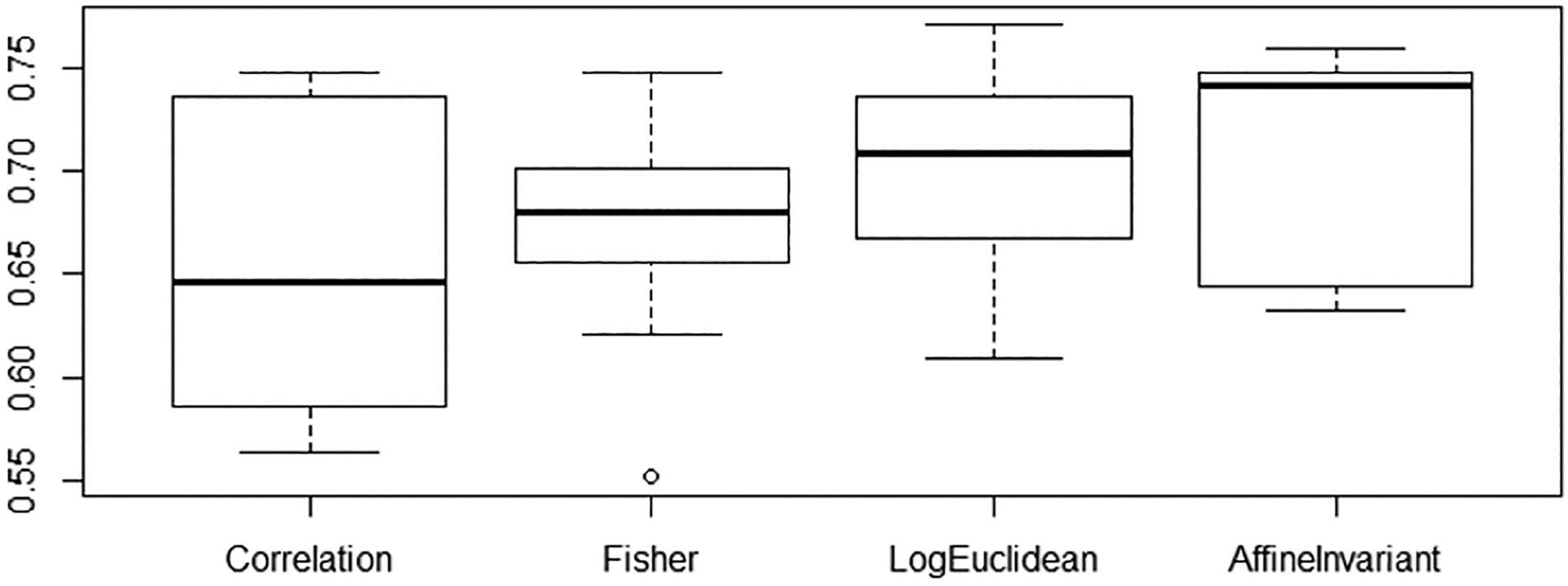
Box plots of the classification accuracy over ten-fold cross-validation.

Fig.3.

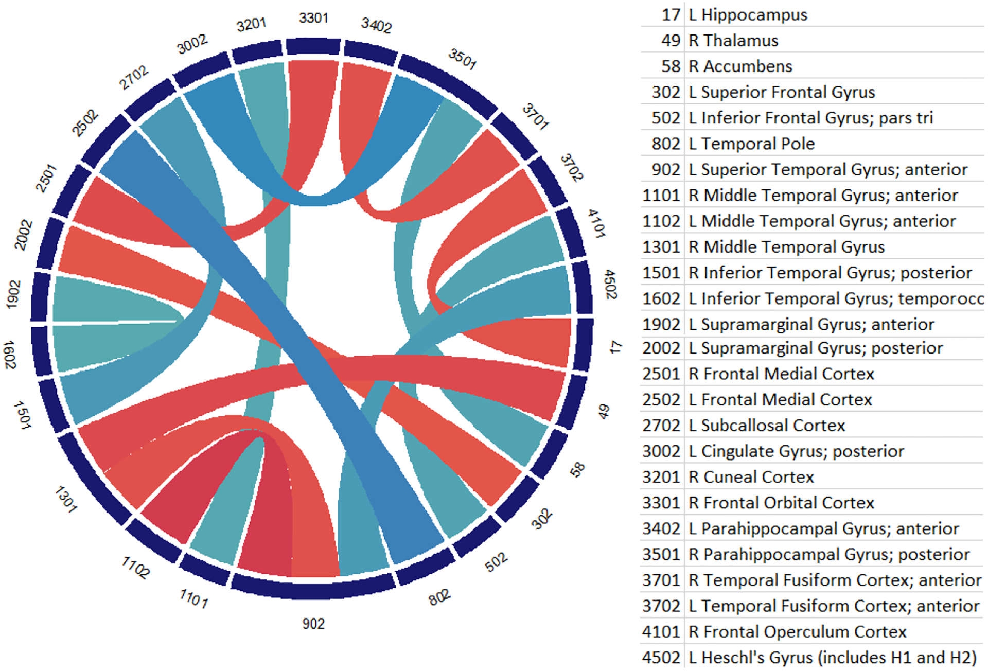
Plot of the connections with highest weights in the classification

Figure 1 is a diagram of the learned weights on the ROIs grouped by subnetworks from [19]–visual, default mode, sensorimotor, auditory, executive control, and frontoparietal networks. The colormap runs from negative values in blue (driving classification toward control) to positive values in red (toward autism). For visualization, very small weights have been filtered. There is evidence of patterns within and between subnetworks. The weights within a subnetwork are simplified to their means within a block. Our results show that control subjects tend to have higher intranetwork connectivity especially within the sensorimotor, executive control, and default mode networks, whereas subjects with ASD have stronger internetwork connectivity, e.g., between the default mode and the sensorimotor networks. This is in agreement with existing literature that the default mode network is not well segregated from other subnetworks for the ASD population [5, 21, 22].

Fig.1.

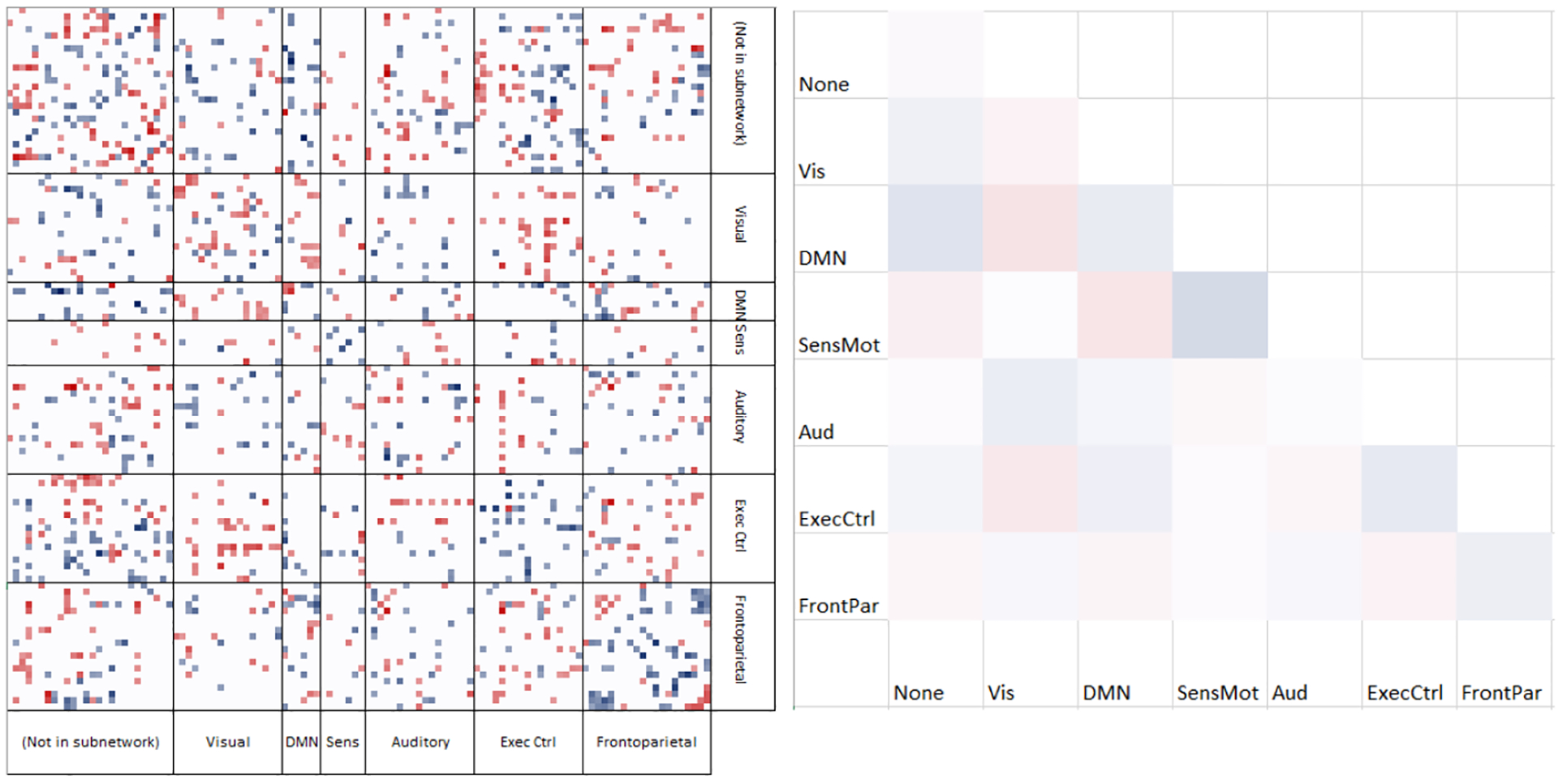
Classification weights grouped by subnetwork

3.2. Regression

To show that the Riemannian features also have predictive power in regression, we compare the performance of log-Euclidean and affine-invariant transformed matrices versus raw correlation matrices in the prediction of autism severity as measured by the ADOS Total score. Though there has been work on doing regression on Riemannian manifolds [6, 14], it has not been applied for ASD analysis. Because regression is more challenging than classification, and some sites lack ADOS scores for control subjects, we limit our analysis to the largest site with a roughly even split of ASD and control subjects that have ADOS Total score. The Utah site has 62 subjects with scores ranging from 0 to 21. Scores below 10 are considered typically developing. We use partial least squares regression (PLS), with the features projected down to one component and regressed to ADOS. It is not trivial to adapt the base point optimization for the NIPALS algorithm in solving PLS. Instead, here we fix the base point to the Fréchet mean. Table 2 shows the root mean squared error (RMSE), R² and Q² coefficient of determination values between Riemannian and baseline correlation matrix features. The R² is computed over the whole data subset, and the Q² value is calculated through a leave-one-out cross-validation (LOOCV) scheme. The plot of true versus predicted ADOS using the Fréchet mean base point is shown in Figure 4. To show the statistical significance of improvement, we do a permutation test. We sum up the absolute value of the residuals of the LOOCV predictions and take the difference of the proposed method from the baseline correlation as the test statistic. Then we do 10000 permutations swapping the predictions between the two classes and sum up the number of times that the differences are greater than our nonpermuted test statistic value. Both log-Euclidean and affine-invariant metrics signicantly improve over the raw and Fisher correlation baselines (also similarly significant by t-test on the RMSE).

Table 2.

Comparison of Riemannian features against baselines in PLS regression

	RMSE	R2	Q2	Raw Corr Improve	Fish Corr Improve
Raw Correlation	6.17	0.631	−0.05	-	-
Fisher Correlation	6.18	0.624	−0.062	-	-
Log-Euclidean	5.42	0.816	0.182	p =0.0112	p =0.0127
Affine-Invariant	5.36	0.837	0.202	p =0.0064	p =0.0069

Fig.4.

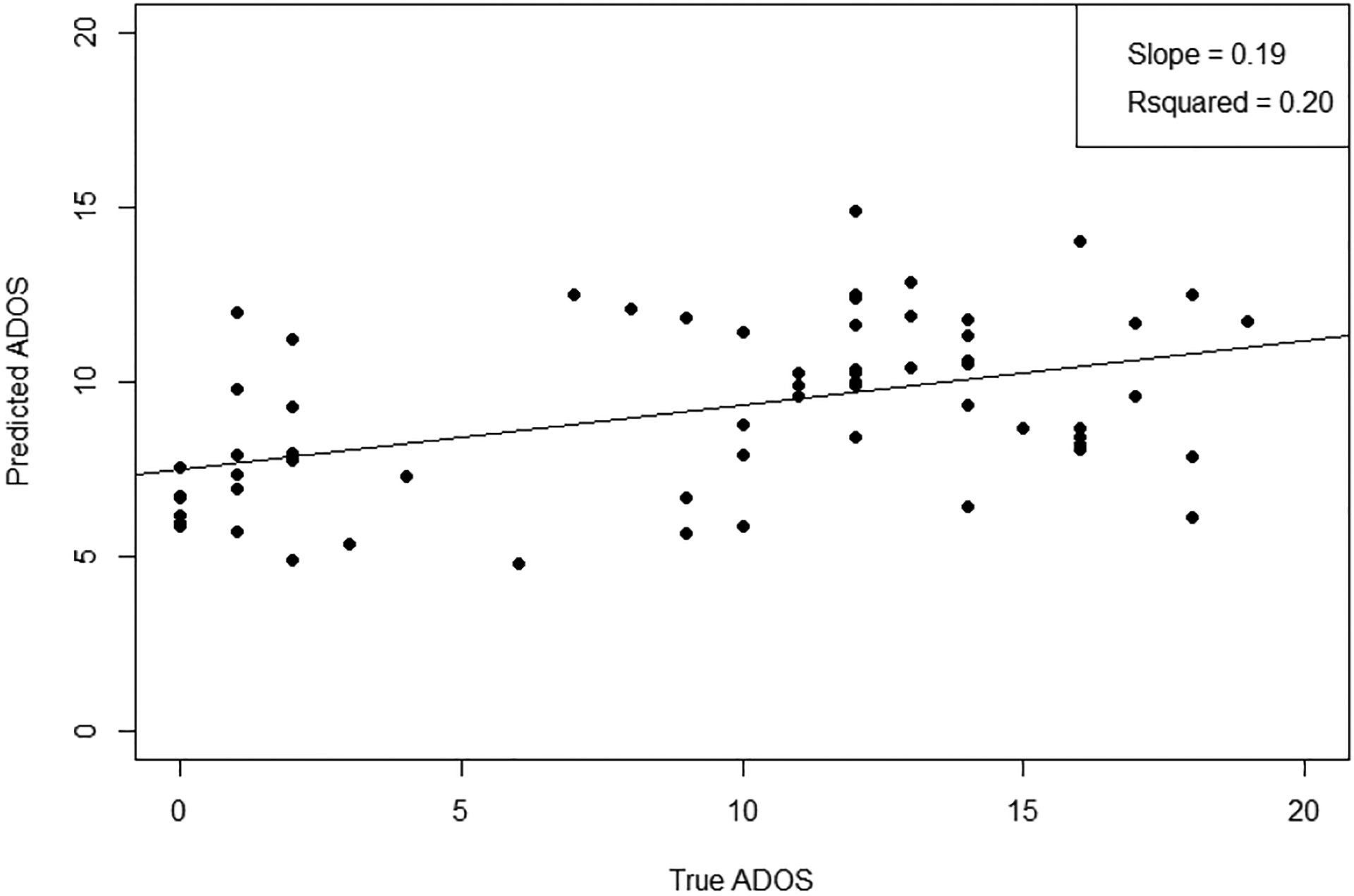
Predicted vs. true ADOS scores for regression under AIM

The regression weights in Figure 5 show similar patterns to the classification results, though not the same. This is expected because the regression data is only a single-site subset. The classification and the regression weights share a correlation of 0.31, reasonably consistent for such high-dimensional data. Summarizing weights into means of each block, we can see the pattern that the intraconnectivity in the default mode and sensorimotor networks drives the regression toward low ADOS scores (control) and interconnectivity between the two networks pushes regression toward high ADOS scores.

Fig.5.

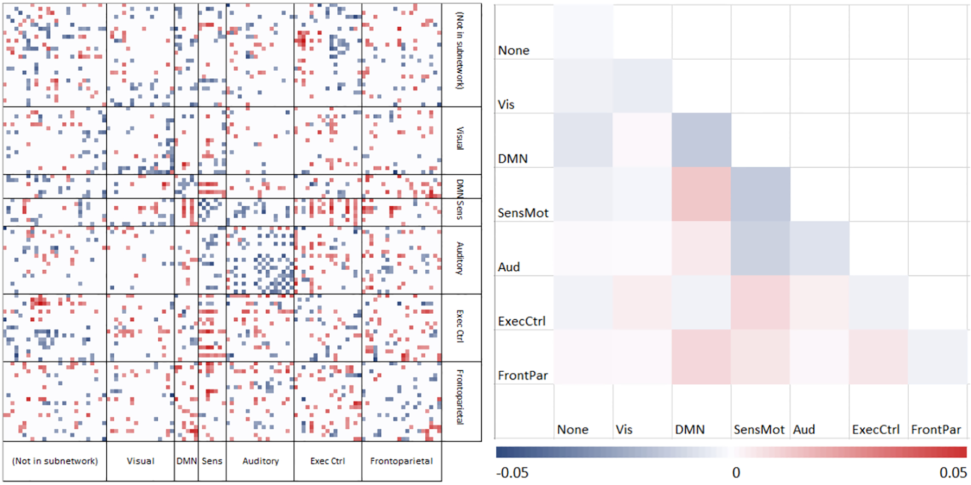
Regression weights grouped by subnetwork

4. Conclusion

In this paper, we have established that the Riemannian representation of SPD matrices is beneficial for the autism classification and regression tasks and comparable in performance to other modern methods. In particular, the results are interpretable under the log-Euclidean metric, whereas the affine-invariant metric leads to high learning performance. For future work, we will compare how the choice of ROI may have an effect on predictions. We will also develop the affine-invariant base point update for other analyses, and study whether it may yield an improvement in performance in a deep neural network.

References

- 1.Abraham A, Milham MP, Di Martino A, Craddock RC, Samaras D, Thirion B, and Varoquaux G. Deriving reproducible biomarkers from multi-site resting-state data: an autism-based example. NeuroImage, 147:736–745, 2017. [DOI] [PubMed] [Google Scholar]
- 2.Anirudh R and Thiagarajan JJ. Bootstrapping graph convolutional neural networks for autism spectrum disorder classification. arXiv preprint arXiv:170407487, 2017. [Google Scholar]
- 3.Arsigny V, Fillard P, Pennec X, and Ayache N. Log-Euclidean metrics for fast and simple calculus on diffusion tensors. Magnetic resonance in medicine, 56(2):411–421, 2006. [DOI] [PubMed] [Google Scholar]
- 4.Arsigny V, Fillard P, Pennec X, and Ayache N. Geometric means in a novel vector space structure on symmetric positive-definite matrices. SIAM journal on matrix analysis and applications, 29(1):328–347, 2007. [Google Scholar]
- 5.Assaf M, Jagannathan K, Calhoun VD, Miller L, Stevens MC, et al. Abnormal functional connectivity of default mode subnetworks in autism spectrum disorder patients. Neuroimage, 53(1):247–256, 2010. [DOI] [PMC free article] [PubMed] [Google Scholar]
- 6.Cornea E, Zhu H, Kim P, Ibrahim JG, and ADNI. Regression models on Riemannian symmetric spaces. Statistical Methodology, 79(2):463–482, 2017. [DOI] [PMC free article] [PubMed] [Google Scholar]
- 7.Craddock C, Benhajali Y, Chu C, Chouinard F, Evans A, Jakab A, Khundrakpam Budhachandra S, Lewis JD, Li Q, Milham M, et al. The neuro bureau preprocessing initiative: open sharing of preprocessed neuroimaging data and derivatives. [Google Scholar]
- 8.Dodero L, Minh HQ, Biagio M San, Murino V, and Sona D. Kernel-based classification for brain connectivity graphs on the Riemannian manifold of positive definite matrices In Biomedical Imaging (ISBI), pages 42–45. IEEE, 2015. [Google Scholar]
- 9.Dvornek NC, Ventola P, Pelphrey KA, and Duncan JS. Identifying autism from resting-state fmri using long short-term memory networks In MLMI, pages 362–370. Springer, 2017. [DOI] [PMC free article] [PubMed] [Google Scholar]
- 10.Fletcher PT, Lu C, Pizer SM, and Joshi S. Principal geodesic analysis for the study of nonlinear statistics of shape. TMI, 23(8):995–1005, 2004. [DOI] [PubMed] [Google Scholar]
- 11.Sólon Heinsfeld A, Franco AR, Craddock RC, Buchweitz A, and Meneguzzi F. Identification of autism spectrum disorder using deep learning and the abide dataset. NeuroImage: Clinical, 17:16–23, 2018. [DOI] [PMC free article] [PubMed] [Google Scholar]
- 12.Huang Z and Van Gool LJ. A Riemannian network for SPD matrix learning. 2017. [Google Scholar]
- 13.Ionescu C, Vantzos O, and Sminchisescu C. Matrix backpropagation for deep networks with structured layers. In ICCV, pages 2965–2973, 2015. [Google Scholar]
- 14.Kim HJ, Adluru N, Collins MD, Chung MK, Bendlin BB, Johnson SC, Davidson RJ, and Singh V. Multivariate general linear models (mglm) on Riemannian manifolds with applications to statistical analysis of diffusion weighted images. In CVPR, pages 2705–2712, 2014. [DOI] [PMC free article] [PubMed] [Google Scholar]
- 15.Meszlényi RJ, Buza K, and Vidnyánszky Zán. Resting state fmri functional connectivity-based classification using a convolutional neural network architecture. Frontiers in neuroinformatics, 11:61, 2017. [DOI] [PMC free article] [PubMed] [Google Scholar]
- 16.Ng B, Dressler M, Varoquaux G, Poline JB, Greicius M, and Thirion B. Transport on Riemannian manifold for functional connectivity-based classification In MICCAI, pages 405–412. Springer, 2014. [DOI] [PubMed] [Google Scholar]
- 17.Parisot S, Ktena SI, Ferrante E, Lee M, Moreno RG, Glocker B, and Rueckert D. Spectral graph convolutions for population-based disease prediction In MICCAI, pages 177–185. Springer, 2017. [Google Scholar]
- 18.Pennec X, Arsigny V, Fillard P, and Ayache N. Fast and simple computations on tensors with log-Euclidean metrics. 2005. [DOI] [PubMed] [Google Scholar]
- 19.Smith SM, Fox PT, Miller KL, et al. Correspondence of the brain’s functional architecture during activation and rest. PNAS, 106(31):13040–13045, 2009. [DOI] [PMC free article] [PubMed] [Google Scholar]
- 20.Varoquaux G, Baronnet F, Kleinschmidt A, Fillard P, and Thirion B. Detection of brain functional-connectivity difference in post-stroke patients using group-level covariance modeling In MICCAI, pages 200–208. Springer, 2010. [DOI] [PubMed] [Google Scholar]
- 21.Weng S, Wiggins JL, Peltier SJ, Carrasco M, Risi S, Lord C, and Monk CS. Alterations of resting state functional connectivity in the default network in adolescents with autism spectrum disorders. Brain research, 1313:202–214, 2010. [DOI] [PMC free article] [PubMed] [Google Scholar]
- 22.Yerys BE, Gordon EM, Satterthwaite D N Abrams, et al. Default mode network segregation and social deficits in autism spectrum disorder: Evidence from non-medicated children. NeuroImage: Clinical, 9:223–232, 2015. [DOI] [PMC free article] [PubMed] [Google Scholar]
- 23.Young J, Lei D, and Mechelli A. Discriminative log-Euclidean kernels for learning on brain networks In CNI, pages 25–34. Springer, 2017. [Google Scholar]