A Spatio‐temporal analysis of COVID‐19 outbreak in Italy

Abstract

Within two weeks from the first detection of the SARS‐CoV‐2 positive patient on 21 February, from Lombardy the disease has spread over every region in Italy. The main objective of this study is to identify spatial effects and spatiotemporal patterns of the outbreak of COVID‐19 in different regions of Italy. Spatial indicators for different periods, as Moran's I, local Moran, LISA clusters, Getis and Ord G, and scatterplots are used for this purpose. Results confirm the great presence of spatial effects as well as changes in spatial regimes between the quarantine and the easing phase. The evidence could be of help for policy‐makers to a proper assessments of health strategies aware of local characteristics.

1. INTRODUCTION

A cluster of severe pneumonia cases from Wuhan, China, came into the recognition of different health professionals in late December 2019 (Feng et al., 2020; Read, Bridgen, Cummings, Ho, & Jewell, 2020; Wang et al., 2020; Wang, Tang, & Wei, 2020). On 31 December 2019, an alert was issued in Wuhan and a notification was made to the World Health Organization (Hui et al., 2020; WHO; Wang, Hornby, Hayden, & Gao, 2020; WHO, 2020). The causative pathogen of this acute pneumonia was identified as the novel coronavirus on 7 January. Further, it was named 2019‐nCoV (Chan, Kok, Zhu, & Chu, 2020; Feng et al., 2020; Tan et al., 2020; Zhu, Zhang, Wang, Li, & Yang, 2020) and later the severe acute respiratory syndrome coronavirus 2 (SARS‐CoV‐2) (Huang et al., 2020; Li et al., 2020). By 23 January total 581 people affected by this virus all over the world and out of which 571 cases were reported from China (WHO, 2020). This figure reached up to 75,748 globally by 20 February.

On that day, the first case of what know as Coronavirus Disease 19 (COVID‐19) was detected in Lombardy. On 11 March, WHO characterized the COVID‐19 as a pandemic. In March, a pandemic wave flowed over the entire North of Italy. As of 15 March 2020, a total of 20,603 confirmed cases with a total of 1,809 deaths were reported in Italy and 153,517 positive cases, with 5,735 deaths were confirmed globally. Within the end of March, Italy has been exposed to a severe outbreak of COVID‐19 (WHO, 2020).

In this paper, we use explorative spatial data analysis (ESDA; Haining, 2003) on Italian COVID‐19 to highlight relevance of local characteristics in management of the pandemic. Spatial effects (i.e., spatial dependence and spatial heterogeneity; Anselin, 1988, 2010) on the whole period and in the quarantine and easing phase are evaluated. Then, starting from this analysis, we consider policies at national and local level to support ad hoc strategies for tackling emergency and prevent sever contagion in more fragile areas.

To provide accurate policy recommendations, we deeply look at both regional (NUTS 2) and province scale for individuating hot and cold spots (NUTS 3). The evidence supports the need for strong commitment of policy‐makers and collaboration at different levels to prevent and avoid disruption of education and economics.

The paper is organized as follows. Section 2 is a brief overview on the regional analysis of COVID‐19 outbreak. Section 3 includes materials and methods. Section 4 shows the results for the whole period under analysis, as well as for two sub‐periods (Phase‐I and Phase‐II). Section 5 concludes the paper.

2. BACKGROUND ON REGIONAL ANALYSIS OF COVID‐19 OUTBREAK

Many authors have tried to outline the spread of COVID‐19. For example, Fanelli and Piazza (2020) have attempted to outline the spread of COVID‐19 through the susceptible, infectious, or recovered (SIR) model. Others have focused on the epidemiological characteristics of the disease in Italy, as the reproduction number and the serial interval of the disease (Cereda et al., 2020; D'Arienzo & Coniglio, 2020; Gatto et al., 2020; Yuan, Li, Lu, & Lu, 2020). Dickson, Espa, Giuliani, Santi, and Savadori (2020) used statistical models to predict outbreaks that are based on both spatial and temporal attributes. They find that also spatial dimension is important to better predict trends over time, as for other others related to viral contagion.

Different spatial models are significant to explain different stages of the diffusion process of an epidemic (Haggett, 1976). According to previous studies (Meng, Wang, Liu, Wu, & Zhong, 2005; Wang, Christakos, Han, & Meng, 2008), researchers have focused on the existence of spatial effects in the diffusion through Moran's I statistic for COVID‐19 and other pathogens in China (Kang, Choi, Kim, & Choi, 2020; Li, Calder, & Cressie, 2007; Zhang, Rao, Wu, Huang, & Dai, 2020). The spatial dynamics of COVID‐19 outbreak have been also tested using global Moran's I statistic for other countries (Bag, Ghosh, Biswas, & Chatterjee, 2020; Rahman, Islam, & Islam, 2020; Shariati, Mesgari, Kasraee, & Jahangiri‐rad, 2020).

Presence of spatial effects (Anselin, 1988) is highly justified in the Italian context. The presence of structural differences and local instabilities in the Peninsula has been empirically shown in many fields. Italy is characterized by a large presence of spatial heterogeneity (Cartone, Casolani, Liberatore, & Postiglione, 2017; Panzera & Postiglione, 2014). This issue calls for deepening the effects of spatial features.

Local peculiarities may also influence the spreading of COVID 19. For example, heterogeneity could lead to different policies and different levels of compliance (Capano, Howlett, Jarvis, Ramesh, & Goyal, 2020). The differences in routines and regulations, as well as differences in health care perception, all highlight the importance of spatial heterogeneity. In fact, the effectiveness of health policies depends on the implementation, which implies to co‐ordinate both national and local levels (Weible, Nohrstedt, Cairney, & Carter, 2020).

In this study, focus on spatial relationships with other indicators of social‐economic characteristics is also under analysis. Investigating those relationships adds to the literature in terms of relevant indicators to be considered by policy‐makers and future research. Bivariate Moran (Anselin, Sridharan, & Gholston, 2007) is used for this aim. Interestingly, the outputs return evidence on lockdown strategies and easing measures that could help to alleviate the trade‐off between healthcare and economic cycle.

3. MATERIALS AND METHODS

3.1. Data

Daily updates from the Ministry of Health and Protezione Civile has been used to calculate indicators connected to COVID‐19 pandemic. Those data are publicly available, and they can be downloaded from https://github.com/pcm-dpc/COVID-19. Additional variables, in terms of socio‐economic indicators, were generally downloaded from the Italian Statistical Bureau (ISTAT, 2015) and Annual Regional Database (ARDECO) of the European Commission.

The time span under analysis starts from the 24th of February to the 26th of June 2020. This was selected to ensure a window including the beginning of the outbreak, the lockdown phase started the 8 of March, the easing that gradually started after the 24 April, as well as reopening (4 May). Our study not only aims at displaying time‐series of new contagions, but also to offer changes in spatial effects over different periods. The time window has been classified into two phases according to the announcement of the Italian Government. Those phases will be referred to as Phase‐I (from the date of first identified COVID‐19 case to 22 April 2020) and Phase‐II (From 23 April to the 26 June).

The gathering process for COVID‐19 official data leads to an accurate choice of the specific indicator. Official statistics for COVID‐19 suffer from bias due to local health strategies. This issue raises both for the number of active cases and for the mortality rate (Saglietto, D'Ascenzo, Zoccai, & De Ferrari, 2020). The Italian official data on the number of daily positive test appears as biased because it does not separate control tests and new patients (Benedetti, Piersimoni, Pignataro, & Vidoli, 2020). The need for more reliable data stresses survey strategies at the regional and provincial levels for improving health policies (Boccia, Ricciardi, & Ioannidis, 2020).

A first solution to this problem is proposed by Bassi, Arbia, and Falorsi (2020), who found that positive cases are underestimated at the nation level. However, after the start of the outbreak, the Italian Ministry of Health introduced guidelines in testing symptomatic subjects (Lorenzoni, Lanera, Azzolina, Berchialla, & Gregori, 2020). In Appendix Figure A1, a plot for the ratio of positive cases on the number of tests is provided. Hence, the number of people affected by the disease has been considered here at the regional level as for other studies (e.g., Rahman, Sadraddin, & Porreca, 2020).

At NUTS 3, the total number of daily contagions has been used and averaged on the time dimension, as data about new contagion cannot be directly retrieved at this level. The particular choice of analyzing NUTS 3 scale is justified by the need of obtaining information at a more granular level.

3.2. Methods

The paper offers an extensive analysis of the role of spatial effects in the COVID 19 pandemic in Italy. We perform a region‐wise and province‐wise spatial explorative analysis, to identify the hot spots or cold spots of COVID 19 in Italy. The evolutions of the spatial dimensions in the different phases is also deepened.

From a more technical point of view, the analysis of spatial patterns and clustering uses widely adopted spatial exploratory indicators. To study spatial dependence, we adopt Moran's I statistic and Moran's scatter plots (Anselin, 1996). Moran's I tell us whether there is spatial dependence or not and it is expressed as follows:

$${\mathrm{I}}_{\mathrm{x}}=\frac{\mathrm{n}}{{\sum }_{\mathrm{i}}{\sum }_{\mathrm{j}}{\mathrm{w}}_{\mathrm{ij}}}\frac{{\sum }_{\mathrm{i}}{\sum }_{\mathrm{j}}{\mathrm{w}}_{\mathrm{ij}}\left({\mathrm{x}}_{\mathrm{j}}-\overline{\mathrm{x}}\right)\left({\mathrm{x}}_{\mathrm{i}}-\overline{\mathrm{x}}\right)}{{\sum }_{\mathrm{i}}{\left({\mathrm{x}}_{\mathrm{i}}-\overline{\mathrm{x}}\right)}^2},$$

where n is the number of regions under analysis, x_i is the value of the variable of interest in the considered region i, $\overline{x}$ is the calculated mean of the selected variable x_i, and w_ij are the entries of a W contiguity matrix indicating spatial proximity between regions. Moran's I can be interpreted in terms of positive global spatial autocorrelation when value of the statistic is above its expected value, i.e. $I>-\frac{1}{n-1}$. Conversely autocorrelation is negative. Correct inference for testing hypothesis can be derived according to Cliff and Ord (1981).

Moran's I, as other spatial indicators, is based on the definition of a contiguity (or connectivity) matrix, generally referred as W. Those matrices are considered as exogenous and they entail spatial connections between units (LeSage & Pace, 2014). Different definition of contiguity matrices may be used, such as contiguity‐based (queen and rook) and distance‐based weights (distance band and k‐nearest neighbour). As the Italian peninsula presents irregular configuration, a k‐nearest neighbours' criterium is selected (Cartone et al., 2017).

In Italy, to only test for spatial dependence would be somewhat misleading (Andreano, Benedetti, & Postiglione, 2017). To consider spatial instabilities we explore spatial heterogeneity. Local indicators of spatial association and related inference (LISA; Anselin, 1995, 1996) are adopted at both levels. In the literature, local Moran can be expressed as a decomposition of global Moran's I:

$$\mathrm{I}{\left(\mathrm{i}\right)}_{\mathrm{x}}=\frac{\mathrm{n}\left({\mathrm{x}}_{\mathrm{i}}-\overline{\mathrm{x}}\right){\sum }_{\mathrm{j}}{\mathrm{w}}_{\mathrm{ij}}\left({\mathrm{x}}_{\mathrm{j}}-\overline{\mathrm{x}}\right)}{{\sum }_{\mathrm{i}}{\left({\mathrm{x}}_{\mathrm{i}}-\overline{\mathrm{x}}\right)}^2},\mathrm{j}\ne \mathrm{i},$$

where n is the number of regions under analysis, x_i is the variable under study, $\overline{x}$ is the calculated mean of the selected variable x_i, and w_ij are the entries of W. Expectation of local Moran is $E\left(I\left(i\right)\right)=\frac{S_i}{n-1}$, where S_i = ∑_iw_ij. Values above the expectation are interpreted as a sign of local positive spatial autocorrelation.

Besides, another well‐known statistic is used to detect for spatial instabilities: the local G (Getis & Ord, 1992). This indicator can be calculated as:

$$G\left(i\right)=\frac{{\sum }_j{w}_{\mathit{ij}}{x}_j}{{\sum }_j{x}_j},j\ne i.$$

Interpretation of this statistic is quite intuitive. A value above $\frac{{\sum }_j{x}_j}{n}$ returns a hotspot, while values under this level indicates cold spots. The derived moments can be used to test the hypothesis of hot and cold spots (Ord & Getis, 1995).

In order to evaluate spatial spillovers generating from other socio‐economic phenomena, bivariate scatter plots are supplied in the results section. Bivariate Moran's scatterplots (Anselin, Syabri, & Kho, 2010) help us to evaluate linear relationships between the spatial lag of a socioeconomic indicators (i.e., the product Wy) and the contagion (e.g., incidence of COVID‐19). The resulting coefficient is calculated equivalently to the univariate Moran's I and it indicates spatial association between variables. Bivariate Moran's I can be written as the following:

$${\mathrm{I}}_{\mathrm{x},\mathrm{y}}=\frac{\mathrm{n}}{{\sum }_{\mathrm{i}}{\sum }_{\mathrm{j}}{\mathrm{w}}_{\mathrm{ij}}}\frac{{\sum }_{\mathrm{i}}{\sum }_{\mathrm{j}}{\mathrm{w}}_{\mathrm{ij}}\left({\mathrm{y}}_{\mathrm{j}}-\overline{\mathrm{y}}\right)\left({\mathrm{x}}_{\mathrm{i}}-\overline{\mathrm{x}}\right)}{{\sum }_{\mathrm{i}}{\left({\mathrm{x}}_2-\overline{\mathrm{x}}\right)}^2},$$

being variable y_j a generic spatially distributed socio‐economic indicator, $\overline{y}$ its mean, and the rest same as above. Bivariate LISA clusters can be also derived accordingly as for the univariate case. Different calculations, diagrammatic representations, and mapping have been made with the help of Microsoft Excel 13, and GeoDa software.

4. RESULTS AND DISCUSSION

4.1. Trends of contagion at the regional level

In the first step, we take a look at the regional trajectories to determine the evolution of the contagion over time. Regions of Italy really differ in terms of the growth of new people infected per day. We divide Italian regions in three main blocks, that is, North, Centre, South and Islands together.

In Figure 1(a), trends for the North are reported for the number of new contagions per day. The plot confirms the very well‐known reality of the sharp situation that has affected Lombardy. We observe an exponential increase that basically leads the region to be the first one in terms of people infected and death toll. For Lombardy, over the first thirty days, the indicators peak at a level of around 2,500 new contagions per day, a quite high figure even considering the regional population (about ten million). Emilia‐Romagna and Veneto positioned quite better, even if they are considered among the top three regions in terms of COVID‐19 contagion. Piemonte peaked quite late and converged towards Lombardy in the second phase. Veneto started a reduction of positive cases after a long plateau during Phase‐II.

FIGURE 1.

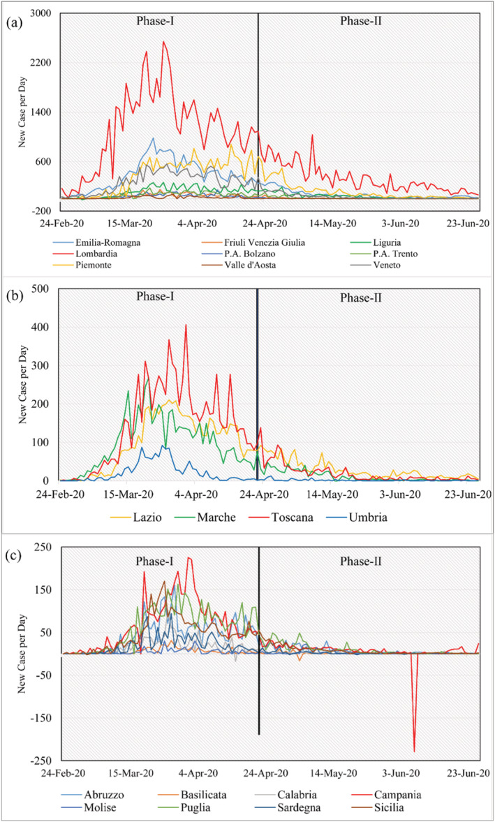
(a) Number of new cases since 24 February for regions located in the north of Italy, and (b) the regions located in the Centre of Italy. (c) Number of new cases since 24 February for regions located in the south of Italy

In the Centre, we observe more homogeneity (Figure 1(b)). The only exception is Umbria, by far the less connected regions to the Northern area. Toscana suffered more than other regions the proximity to Lombardy and peaked around 400 per day. Lazio, which includes an airport hub (Roma Fiumicino), resulted in a moderate number of new cases per day compared to Lombardy despite the elevated number of international connections.

Regions in the South and islands (Figure 1(c)), reached a significantly lower level. Among these, Campania and Puglia got worse figures, a circumstance that is likely due to both population density and a deeper connection with the North. Less inhabited areas like Molise and Basilicata reported only slight numbers of contagion. Regarding the two islands, they peaked at the beginning of April.

As it can be observed in Figure 1(c), Campania shows a minimum during May, which is connected to the presence of people previously considered as infected by COVID19 and later discarded from the count. This point also remarks the necessity of considering data with great detail.

Comparing the three plots, geographical differences are evident. Lombardy represents the epicenter of the pandemic. However, local peculiarities suggest a deeper analysis of spatial effects that will be addressed in the following sections.

4.2. Spatiotemporal analyses at regional level

Spatial effects for the whole pandemic period can be represented by the LISA map along with Moran's scatter plots (Figure 2). A K = 5 row‐standardized k‐nearest neighbours connectivity matrix is used for those calculations.

FIGURE 2.

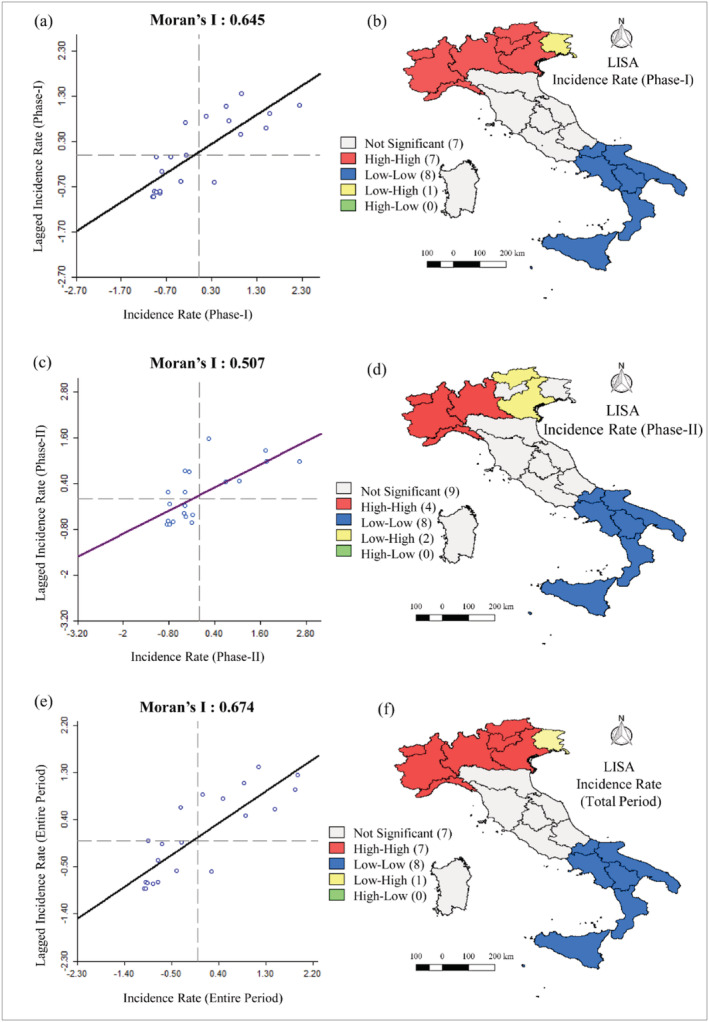
Regional level spatial dependency and clustering of incidence rate in phase I (a) & (b), phase II (c) & (d) and entire period (e) & (f)

In this context, local instabilities are detected for high‐high, low‐low, and low‐high, which can be observed in Italy. The regions in the Northern part of the country (Valle d'Aosta, Piemonte, Liguria, Veneto, Lombardy, Trento, and Bolzano) exposed significantly high prevalence. Only one region situated at the extreme North‐East side, Friuli Venezia Giulia, shows a low prevalence of the disease. The regions in the South (Sicilia, Calabria, Basilicata, Puglia, Campania, and Molise) exhibit a cluster of relatively low prevalence rates. Friuli Venezia Giulia and Trento show insignificant spatial association, while Bolzano and Veneto are found to control the disease especially in Phase‐II. Four regions (Valle d'Aosta, Piemonte, Liguria, Lombardy) indicate a high prevalence rate with high spatial association during Phase II. The low‐low cluster in the southern portion remains stable between phases‐II. The need for scrutinizing spatial differences at a higher resolution leads us to a focus on NUTS 3 in the following section.

4.3. Spatiotemporal analyses at province level

For NUTS 3, the indicator is calculated as an average over the period of the total amount of infected people per day. This quantity is normalized on the total province population of 2019. In Figure 3(a) quantile maps for this indicator are shown.

FIGURE 3.

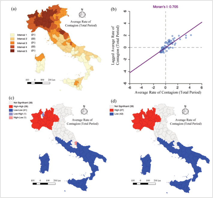
(a) Quintile map of average contagion rate from 24 February to the 30 July at province level, (b) Moran scatterplot, and (c) LISA cluster map (d) hot spot and cold spot by Getis‐Ord G for the average of the total case per day from the 24 February to the 30th of July at province level

We have made the spatial analysis for the entire period, along with two phases of pandemic outbreak separately to offer insights into the spatiotemporal dynamics of the COVID‐19 outbreak in Italy. At this level, all analyses are performed considering a row‐standardized k‐nearest neighbours connectivity matrix with k = 7.

The level of spatial dependence calculated by Moran's I is at 0.705 (Figure 3(b)). In fact, the level of commuting and transportation has been quite high during the lockdown phase, due to basic needs, trade flows, and workers commuting for key sectors.

Looking at the LISA cluster map in Figure 3(c), Italy is evidently split into three different zones. Central provinces result to be not significant in terms of Local Moran's I, being neither high‐high cluster nor low‐low (5% significance).

The North results itself into two different areas, the North‐East and North‐West. In fact, Veneto and Lombardy adopted two very different strategies in tackling the contagion of COVID‐19. If Lombardy went for a more integrated strategy, Veneto adopted very localized actions to track and isolate municipalities. This brought only few provinces, as for the case Padua, to be in the high‐high cluster. Other provinces were successfully isolated from the rest of the region.

It is interesting to notice how Pescara (Abruzzo, on the Adriatic coast) is in the high‐low cluster and it configurates as a spatial outlier. In fact, this province is integrated with Northern regions, being the most productive and economically developed compared to the rest of Abruzzo. Those issues justify NUTS 3 level of analysis, as the regional level (NUTS 2) may be too high scale.

After performing spatial analysis for the whole period, we move a step ahead by considering the two periods, Phase‐I and Phase‐II. Officially, Phase‐II started the 4 May, however, two days after the government decree (22 April) many regions decided to ease lockdown restrictions. Hence, we include this time window into the second phase. In Figure 4(a) and (b), quantile maps show slight differences in Province between Phase‐I and Phase‐II (Apulia and Campania). Intuitively, this is due to natives returning from working places in Lombardy.

FIGURE 4.

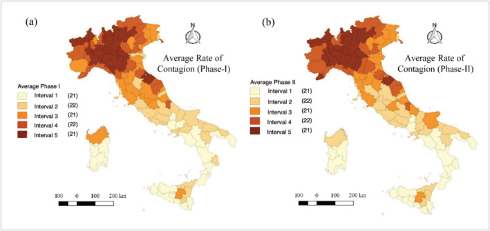
Quantile maps for or the average of the total case per day over (a) “phase‐I" and (b) “phase‐II" at province level

In Figure 5, we appreciate an increase in the level of Moran's between the two different periods, going from the 0.633 to the 0.728. This may be caused by increasing interconnections at the national level, starting from rising commuting within regions, access to second houses, progressive reopening of commerce, and re‐opening of tourism structures after easing.

FIGURE 5.

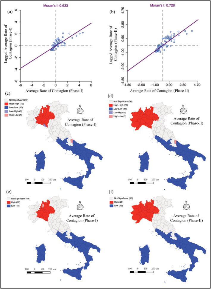
Global Moran and Moran scatterplot for (a) “phase‐I”, and (b) “phase‐II”, local Moran and LISA clusters for (c) “phase‐I”, (d) “phase‐II”, and hot and cold spots calculated via Getis‐Ord G for (e) “phase‐I”, (f) phase‐II

We also compare LISA cluster maps (Figure 5(c) and 5(d)). LISA cluster maps return major differences between the two periods. The high‐high cluster expanded during Phase‐II, especially in the North‐West (Figure 5(d)). This circumstance may be linked to the high interconnections between the Provinces of Emilia, Lombardy, and Piedmont. Those regions are very dependent on each other for services, manufacturing supplies, and commuting flows (De Dominicis, Arbia, & De Groot, 2013). In Veneto, only two provinces entered the high‐high cluster in Phase‐II. This detail supports again localized lockdowns, together with massive testing (Valent et al., 2020).

Figures 5(c) and 5(d) report a substantially invariant picture in the South. Only a slight enlargement of the low‐low cluster can be appreciated towards the Southern provinces of Tuscany (as for the case of Grosseto). On the Adriatic coast, Abruzzo is split between a low‐low (Chieti) and high‐low (Pescara). Once more, local peculiarities appear as extremely important to offer precise policy support.

In Figure 5(e) and 5(f) a comparison between different periods is shown using local Getis‐Ord G. From the Figure 5(e) and 5(f), the hot spot of contagion is again limited around Lombardy. LISA indicators confirm that economically most developed areas in the Country are more likely to be affected by COVID 19.

Results at the province level could be used as additional evidence to support local ad hoc policies that can help coherence between national, regional, and local. Moving from a complete lockdown strategy to more localized and precise restrictions could be considered as a reasonable option. However, local policies have to be co‐ordinated from the national Government to rationalize too heavy interregional interconnections that could ignite contagion in less developed areas. A strong case in support of this view is represented by South Korea (Her, 2020).

A set of possible ad hoc policy recommendations is summarized in Table 1. As shown, different situations lead to the definition of different actions, ranging from emergency to prevention. Recommendations strongly differ on a spatial dimension in Italy. They range from dealing with emergency issue in the North (e.g., lockdown and social distancing) and actions to prevent from widespread in the more fragile locations in the South (e.g., improving transportation and preventing intensive care infrastructure). Indeed, local and national decision‐makers could benefit from the analyses for more coherent healthcare, transportation, and economics policies.

TABLE 1.

Policy recommendations for health, economics, transportation, and education for different COVID‐19 LISA clusters in Italy

Zone	Strategies	Policy recommendation
Hot spots	Emergency response	• door to door mass testing; • strictly separate management of COVID and non‐COVID patients in hospitals; • partial lockdown and social distancing; • special health policies for frontline workers; • severe restriction in tourism; • online education; • subsides on local business.
Insignficant areas	Response and recovery	• social distancing; • avoidance of mass gathering in social events; • guidelines on health management and transportations. • planning peculiar strategies for economic and financial sustainability; • blended strategies for teaching (classrooms/remote).
Cold spots	Protection	• investments on intensive care units; • attention to inter‐province or inter‐regional transport; • restrictions to north–south connections or international migration; • emphasis on local businesses; • support remote teaching and IT facilities for schools and higher education.

4.4. Spatial effects and relations to local development

In the previous sections, COVID 19 contagion is found to be influenced by the presence of spatial effects. To get a more extensive picture of the spatial characteristics, we also perform analysis considering variables linked to development. The analysis is carried on using the bivariate Moran's I and bivariate LISA techniques.

At the regional level, the spatial correlation between HDI and incidence rate shows a significant positive relationship (Moran's I = 0.517 and significant) between the two (Figure 6(a)). The positive spatial correlation of incidence rate with per capita income (Moran's I = 0.652). The spatial correlation of other two dimensions of HDI, life expectancy and mean year of schooling with the incidence rate remain very low but positive. These results suggest how more developed regions have been majorly affected by COVID‐19.

FIGURE 6.

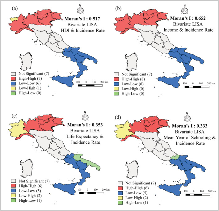
Spatial correlation of (a) HDI, and the dimensions of HDI (b) income (c) life expectancy and (d) mean year of schooling with the incidence rate of COVID‐19 during the whole period

Due to lack of extensive HDI data for provinces, a bivariate LISA is offered at this level with reference to the GDP per capita in purchase power standard (PPS; Figure 7). The highest positive spatial correlation in the North provinces stresses the link between economic development and COVID‐19. The result may be connected to the presence of more connections with neighbouring regions in the North, which causes higher contact rates.

FIGURE 7.

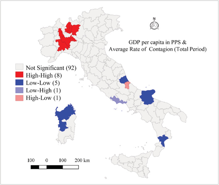
Bivariate LISA between GDP per capita in PPS and average of total case per day at province level. elaboration made over the whole period

Even if this brief analysis cannot be considered as exhaustive, it offers important results for policy‐makers. First, the modeling of COVID‐19 cannot exclude for the presence of spatial effects, especially for the presence of local instabilities. Second, policy‐makers have to consider both spatial dependence and spatial heterogeneity, which may change relations over space.

4.5. The MAUP effect in spatial analyses of COVID‐19 outbreak

A relevant topic that emerges when studying different spatial resolution regards the problem of the modifiable areal unit problem (MAUP; Openshaw & Taylor, 1979). The MAUP problem is likely to bring puzzling interpretation and bring differences in correlations between variables at different levels (Arbia, Benedetti, & Espa, 1996). MAUP issues can create confusion between analysis at different levels and support opposite strategies. This would not help coherence between policies at regional and national level, as for the case of health.

In this study, we observe as the level of Global Moran's I keep constant in Phase‐I. Nevertheless, at the province level, Global Moran's I is higher in the second phase. Conversely, the regional level show opposite results, being autocorrelation lower in Phase‐II. In fact, autocorrelation keeps quite stable between spatial scales during lockdown, when regional barriers are present. While easing, the discrepancy between different resolutions increases and spatial autocorrelation raises at the finer resolution. This circumstance is likely assumable due to progressive return to frequent interconnections. Hence, this feature justifies a closer look to data at the province level.

Concerning spatial heterogeneity and clustering procedures, the use of a high resolution has been also recommended for the case of Italy (Cartone & Postiglione, 2020). In fact, the information on this spatial effect could be lost or distorted at aggregated levels, so that a higher resolution helps accuracy of clustering routines.

5. CONCLUDING REMARKS

In this paper, we evaluate spatial effects related to COVID‐19 contagion, both at the regional and province levels. To do so, we exploit ESDA indicators for both detecting spatial dependence and spatial heterogeneity. We rely on contagion data over different periods to evaluate spatial clusters. Explorative statistics appear quite informative to the need of evaluating critical situations, highlight local pressure on the health system, and develop localized policies.

Analysis of spatial effects leads to a more complete information on the dynamic of pandemic in Italy. The presence of local instability and differences in the factor influencing hot spots should be carefully considered in the policy‐making. Localized lockdowns could be more sustainable in terms of economic activities compared to national‐level strategies. In fact, more specific policies are needed to control COVID‐19 with accelerating economy in the presence of clusters.

A deeper knowledge of the geography of contagion could also help higher co‐ordination between national and local policies. This aspect is extremely relevant to maintain health standards, avoid social tensions, and reduce job disruption. Results should be integrated in future lines thanks to accurate spatial modelling and strong consideration of the effects of spatial scale due to MAUP.

APPENDIX A.

FIGURE A1.

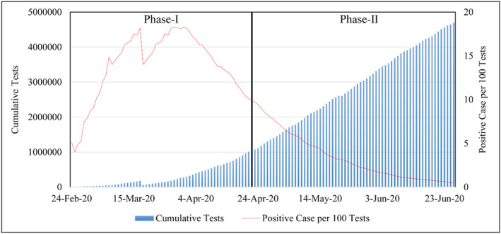
Ratio of number of positive cases on the total number of tests performed every day at the national level

Ghosh P, Cartone A. A Spatio‐temporal analysis of COVID‐19 outbreak in Italy. Reg Sci Policy Pract. 2020;12:1047–1062. 10.1111/rsp3.12376

REFERENCES

- Andreano, M. S. , Benedetti, R. , & Postiglione, P. (2017). Spatial regimes in regional European growth: An iterated spatially weighted regression approach. Quality and Quantity, 51(6), 2665–2684. 10.1007/s11135-016-0415-1 [DOI] [Google Scholar]
- Anselin, L. (1988). Lagrange multiplier test diagnostics for spatial dependence and spatial heterogeneity. Geographical Analysis, 20, 1–17. [Google Scholar]
- Anselin, L. (1995). Local indicators of spatial association—LISA. Geographical Analysis, 27, 93–115. [Google Scholar]
- Anselin, L. (1996). The Moran scatterplot as an ESDA tool to assess local instability in spatial association In Fischer M., Scholten H., & Unwin D. (Eds.), Spatial analytical perspectives on GIS in environmental and socio‐economic sciences (pp. 111–125). London: Taylor and Francis. [Google Scholar]
- Anselin, L. (2010). Thirty years of spatial econometrics. Papers in Regional Science, 89(1), 3–25. 10.1111/j.1435-5957.2010.00279.x [DOI] [Google Scholar]
- Anselin, L. , Sridharan, S. , & Gholston, S. (2007). Using exploratory spatial data analysis to leverage social indicator databases: The discovery of interesting patterns. Social Indicators Research, 82, 287–309. 10.1007/s11205-006-9034-x [DOI] [Google Scholar]
- Anselin, L. , Syabri, I. , & Kho, Y. (2010). GeoDa: An introduction to spatial data analysis In Fischer M. M. & Getis A. (Eds.), Handbook of applied spatial analysis: Software Tools, Methods and Applications (pp. 73–89). Berlin: Springer. [Google Scholar]
- Arbia, G. , Benedetti, R. , & Espa, G. (1996). Effects of the MAUP on image classification. Geographical Systems, 3, 123–141. [Google Scholar]
- Bag, R. , Ghosh, M. , Biswas, B. , & Chatterjee, M. (2020). Understanding the spatio‐temporal pattern of COVID‐19 outbreak in India using GIS and India's response in managing the pandemic. Regional Science Policy and Practice. 10.1111/rsp3.12359 [DOI] [PMC free article] [PubMed] [Google Scholar]
- Bassi, F. , Arbia, G. , & Falorsi, P. D. (2020). Observed and estimated prevalence of Covid‐19 in Italy: How to estimate the total cases from medical swabs data. The Science of the Total Environment, 142799 10.1016/j.scitotenv.2020.142799 [DOI] [PMC free article] [PubMed] [Google Scholar]
- Benedetti, R. , Piersimoni, F. , Pignataro, G. , & Vidoli, F. (2020). The identification of spatially constrained homogeneous clusters of Covid‐19 transmission in Italy. Regional Science Policy and Practice. 10.1111/rsp3.12371 [DOI] [Google Scholar]
- Boccia, S. , Ricciardi, W. , & Ioannidis, J. P. (2020). What other countries can learn from Italy during the COVID‐19 pandemic. JAMA Internal Medicine, 180(7), 927–928. 10.1001/jamainternmed.2020.1447 [DOI] [PubMed] [Google Scholar]
- Capano, G. , Howlett, M. , Jarvis, D. S. , Ramesh, M. , & Goyal, N. (2020). Mobilizing policy (in) capacity to fight COVID‐19: Understanding variations in state responses. Policy and Society, 39, 285–308. 10.1080/14494035.2020.1787628 [DOI] [PMC free article] [PubMed] [Google Scholar]
- Cartone, A. , Casolani, N. , Liberatore, L. , & Postiglione, P. (2017). Spatial analysis of grey water in Italian cereal crops production. Land Use Policy, 68, 97–106. 10.1016/j.landusepol.2017.06.024 [DOI] [Google Scholar]
- Cartone, A. , & Postiglione, P. (2020). Principal component analysis for geographical data: the role of spatial effects in the definition of composite indicators. Spatial Economic Analysis, 1–22. 10.1080/17421772.2020.1775876 [DOI] [Google Scholar]
- Cereda, D. , Tirani, M. , Rovida, F. , Demicheli, V. , Ajelli, M. , Poletti, P. , … Merler, S. (2020). The early phase of the COVID‐19 outbreak in Lombardy, Italy. https://arxiv.org/ftp/arxiv/papers/2003/2003.09320.pdf
- Chan, J. F. W. , Kok, K. H. , Zhu, Z. , & Chu, H. (2020). Genomic characterization of the 2019 novel human‐pathogenic coronavirus isolated from a patient with atypical pneumonia after visiting Wuhan. Emerging Microbes & Infections, 9, 221–236. 10.1080/22221751.2020.1719902 [DOI] [PMC free article] [PubMed] [Google Scholar]
- Cliff, A. D. , & Ord, J. K. (1981). Spatial processes: Models & applications. London: Taylor & Francis. [Google Scholar]
- D'Arienzo, M. , & Coniglio, A. (2020). Assessment of the SARS‐CoV‐2 basic reproduction number, R0, based on the early phase of COVID‐19 outbreak in Italy. Biosafety and Health, 2, 57–59. 10.1016/j.bsheal.2020.03.004 [DOI] [PMC free article] [PubMed] [Google Scholar]
- De Dominicis, L. , Arbia, G. , & De Groot, H. L. (2013). Concentration of manufacturing and service sector activities in Italy: Accounting for spatial dependence and firm size distribution. Regional Studies, 47(3), 405–418. 10.1080/00343404.2011.579593 [DOI] [Google Scholar]
- Dickson, M. M. , Espa, G. , Giuliani, D. , Santi, F. , & Savadori, L. (2020). Assessing the effect of containment measures on the spatio‐temporal dynamic of COVID‐19 in Italy. Nonlinear Dynamics, 101, 1833–1864. 10.1007/s11071-020-05853-7 [DOI] [PMC free article] [PubMed] [Google Scholar]
- Fanelli, D. , & Piazza, F. (2020). Analysis and forecast of COVID‐19 spreading in China, Italy and France. Chaos, Solitons and Fractals, 134, 1–5. 10.1016/j.chaos.2020.109761 [DOI] [PMC free article] [PubMed] [Google Scholar]
- Feng, Z. , Li, Q. , Zhang, Y. , Wu, Z. , Dong, X. , Ma, H , … The Novel Coronavirus Pneumonia Emergency Response Epidemiology Team . (2020). The epidemiological characteristics of an outbreak of 2019 novel coronavirus diseases (COVID‐19) — China, 2020. China CDC Weekly, 2(x), 1–10. [PMC free article] [PubMed] [Google Scholar]
- Gatto, M. , Bertuzzo, E. , Mari, L. , Miccoli, S. , Carraro, L. , Casagrandi, R. , & Rinaldo, A. (2020). Spread and dynamics of the COVID‐19 epidemic in Italy: Effects of emergency containment measures. PNAS Latest Articles, 117, 10484–10491. 10.1073/pnas.2004978117 [DOI] [PMC free article] [PubMed] [Google Scholar]
- Getis, A. , & Ord, J. K. (1992). The analysis of spatial association by use of distance statistics. Geographical Analysis, 24(3), 189–206. 10.1111/j.1538-4632.1992.tb00261.x [DOI] [Google Scholar]
- Haggett, P. (1976). Hybridizing alternative models of an epidemic diffusion process. Human Health Problems: Spatial Perspectives, 52(2), 136–146. [Google Scholar]
- Haining, R. (2003). Spatial data analysis: Theory and practice. Cambridge: Cambridge University Press; 10.1017/CBO9780511754944 [DOI] [Google Scholar]
- Her, M. (2020). How is COVID‐19 affecting South Korea? What is our current strategy? Disaster Medicine and Public Health Preparedness, 1–3. 10.1017/dmp.2020.69 [DOI] [PMC free article] [PubMed] [Google Scholar]
- Huang, C. , Wang, Y. , Li, X. , Ren, L. , Zhao, J. , Hu, Y. , … Cao, B. (2020). Clinical features of patients infected with 2019 novel coronavirus in Wuhan, China. Lancet, 395, 497–506. 10.1016/S0140-6736(20)30183-5 [DOI] [PMC free article] [PubMed] [Google Scholar]
- Hui, D. S. , Azhar, E. I. , Madani, T. A. , Ntoumi, F. , Kock, R. , & Dar, O. (2020). The continuing 2019‐nCoV epidemic threat of novel coronaviruses to global health: The latest 2019 novel coronavirus outbreak in Wuhan, China. International Journal of Infectious Diseases, 91(2020), 264–266. 10.1016/j.ijid.2020.01.009 [DOI] [PMC free article] [PubMed] [Google Scholar]
- ISTAT . (2015). Il Benessere Equo e Sostenibile in Italia. Rapporto 2015 Roma: Istituto Nazionale di Statistica. [Google Scholar]
- Kang, D. , Choi, H. , Kim, J. H. , & Choi, J. (2020). Spatial epidemic dynamics of the COVID‐19 outbreak in China. International Journal of Infectious Diseases, 94, 96–102. 10.1016/j.ijid.2020.03.076 [DOI] [PMC free article] [PubMed] [Google Scholar]
- LeSage, J. P. , & Pace, R. K. (2014). The biggest myth in spatial econometrics. Econometrics, 2(4), 217–249. 10.3390/econometrics2040217 [DOI] [Google Scholar]
- Li, H. , Calder, C. A. , & Cressie, N. (2007). Beyond Moran's I: Testing for spatial dependence based on the spatial autoregressive model. Geographical Analysis, 39(4), 357–375. 10.1111/j.1538-4632.2007.00708.x [DOI] [Google Scholar]
- Li, Q. , Guan, X. , Wu, P. , Wang, X. , Zhou, L. , & Tong, Y. (2020). Early transmission dynamics in Wuhan, China, of novel coronavirus– Infected pneumonia. The New England Journal of Medicine, 382(13), 1199–1207. 10.1056/NEJMoa2001316 [DOI] [PMC free article] [PubMed] [Google Scholar]
- Lorenzoni, G. , Lanera, C. , Azzolina, D. , Berchialla, P. , & Gregori, D. (2020). Is a more aggressive COVID‐19 case detection approach mitigating the burden on ICUs? Some reflections from Italy. Critical Care, 24, 1–2. [DOI] [PMC free article] [PubMed] [Google Scholar]
- Meng, B. , Wang, J. , Liu, J. , Wu, J. , & Zhong, E. (2005). Understanding the spatial diffusion process of severe acute respiratory syndrome in Beijing. Public Health, 119(12), 1080–1087. 10.1016/j.puhe.2005.02.003 [DOI] [PMC free article] [PubMed] [Google Scholar]
- Openshaw, S. , & Taylor, P. J. (1979). A million or so correlation coefficients: Three experiments on the modifiable areal unit problem In Wrigley N. (Ed.), Statistical applications in spatial sciences (pp. 127–144). London: Pion. [Google Scholar]
- Ord, J. K. , & Getis, A. (1995). Local spatial autocorrelation statistics: Distributional issues and an application. Geographical Analysis, 27, 286–306. 10.1111/j.1538-4632.1995.tb00912.x [DOI] [Google Scholar]
- Panzera, D. , & Postiglione, P. (2014). Economic growth in Italian NUTS 3 provinces. The Annals of Regional Science, 53(1), 273–293. 10.1007/s00168-014-0628-y [DOI] [Google Scholar]
- Rahman, B. , Sadraddin, E. , & Porreca, A. (2020). The basic reproduction number of SARS‐CoV‐2 in Wuhan is about to die out, how about the rest of the world? Reviews in Medical Virology, 30, e2111 10.1002/rmv.2111 [DOI] [PMC free article] [PubMed] [Google Scholar]
- Rahman, R. , Islam, A. H. M. H. , & Islam, N. (2020). Geospatial modelling on the spread and dynamics of 154 day outbreak of the novel coronavirus (COVID‐19) pandemic in Bangladesh towards vulnerability zoning and management approaches. Modeling Earth Systems and Environment. 10.1007/s40808-020-00962-z [DOI] [PMC free article] [PubMed] [Google Scholar]
- Read, J. M. , Bridgen, J. R. E. , Cummings, D. A. T. , Ho, A. , & Jewell, C. P. (2020). Novel coronavirus 2019‐nCoV: Early estimation of epidemiological parameters. MedRxiv. 10.1101/2020.01.23.20018549 [DOI] [PMC free article] [PubMed] [Google Scholar]
- Saglietto, A. , D'Ascenzo, F. , Zoccai, G. B. , & De Ferrari, G. M. (2020). COVID‐19 in Europe: The Italian lesson. Lancet, 395(10230), 1110–1111. 10.1016/S0140-6736(20)30690-5 [DOI] [PMC free article] [PubMed] [Google Scholar]
- Shariati, M. , Mesgari, T. , Kasraee, M. , & Jahangiri‐rad, M. (2020). Spatiotemporal analysis and hotspots detection of COVID‐19 using geographic information system (march and April 2020). Journal of Environmental Health Science and Engineering. 10.1007/s40201-020-00565-x [DOI] [PMC free article] [PubMed] [Google Scholar]
- Tan, W. , Zhao, X. , Ma, X. J. , Wang, W. L. , Niu, P. , Xu, W. , … Wu, G. (2020). A novel coronavirus genome identified in a cluster of pneumonia cases—Wuhan, China 2019−2020. China CDC Weekly, 2(4), 61–62. http://weekly.chinacdc.cn/en/article/ccdcw/2020/4/61. 10.46234/ccdcw2020.017 [DOI] [PMC free article] [PubMed] [Google Scholar]
- Valent, F. , Gallo, T. , Mazzolini, E. , Pipan, C. , Sartor, A. , Merelli, M. , … Tascini, C. (2020). A cluster of COVID‐19 cases in a small Italian town: A successful example of contact tracing and swab collection. Clinical Microbiology and Infection, 26, 1112–1114. 10.1016/j.cmi.2020.04.028 [DOI] [PMC free article] [PubMed] [Google Scholar]
- Wang, C. , Hornby, P. W. , Hayden, F. G. , & Gao, G. F. (2020). A novel coronavirus outbreak of global health concern. Lancet, 395, 470–473. 10.1016/S0140-6736(20)30185-9 [DOI] [PMC free article] [PubMed] [Google Scholar]
- Wang, C. , Liu, Z. , Chen, Z. , Huang, X. , Xu, M. , He, T. , & Zhang, Z. (2020). The establishment of reference sequence for SARS‐CoV‐2 and variation analysis. Journal of Medical Virology, 92, 667–674. 10.1002/jmv.25762 [DOI] [PMC free article] [PubMed] [Google Scholar]
- Wang, J. F. , Christakos, G. , Han, W. G. , & Meng, B. (2008). Data‐driven exploration of ‘spatial pattern‐time process‐driving forces’ associations of SARS epidemic in Beijing, China. Journal of Public Health, 30(3), 234–244. 10.1093/pubmed/fdn023 [DOI] [PMC free article] [PubMed] [Google Scholar]
- Wang, W. , Tang, J. , & Wei, F. (2020). Updated understanding of the outbreak of 2019 novel coronavirus (2019‐nCoV) in Wuhan, China. Journal of Medical Virology, 92, 441–447. 10.1002/jmv.25689 [DOI] [PMC free article] [PubMed] [Google Scholar]
- Weible, C. M. , Nohrstedt, D. , Cairney, P. , & Carter, D. P. (2020). COVID‐19 and the policy sciences: Initial reactions and perspectives. Political Science, 53, 225–241. 10.1007/s11077-020-09381-4 [DOI] [PMC free article] [PubMed] [Google Scholar]
- World Health Organization . (2020). Coronavirus disease 2019 (COVID‐19) situation Report‐55. March 15. URL: https://www.who.int/docs/default-source/coronaviruse/situation-reports/20200315-sitrep-55-covid-19.pdf?sfvrsn=33daa5cb_8
- Yuan, J. , Li, M. , Lu, G. , & Lu, Z. K. (2020). Monitoring transmissibility and mortality of COVID‐19 in Europe. International Journal of Infectious Diseases, S1201–9712(20)30182‐X, 95, 311–315. 10.1016/j.ijid.2020.03.050 [DOI] [PMC free article] [PubMed] [Google Scholar]
- Zhang, X. , Rao, H. , Wu, Y. , Huang, Y. , & Dai, H. (2020). Comparison of spatiotemporal characteristics of the COVID‐19 and SARS outbreaks in mainland China. BMC Infectious Diseases, 20(805), 1–7. 10.1186/s12879-020-05537-y [DOI] [PMC free article] [PubMed] [Google Scholar]
- Zhu, N. , Zhang, D. , Wang, W. , Li, X. W. , & Yang, B. (2020). A novel coronavirus from patients with pneumonia in China, 2019. The New England Journal of Medicine, 382, 727–733. 10.1056/nejmoa2001017 [DOI] [PMC free article] [PubMed] [Google Scholar]