Entropy Scaling of Viscosity – I: A Case Study of Propane

Abstract

In this work, a broadly-applicable and simple approach for building high accuracy viscosity correlations is demonstrated for propane. The approach is based on the combination of a number of recent insights related to the use of residual entropy scaling, especially a new way of scaling the viscosity for consistency with the dilute-gas limit.

With three adjustable parameters in the dense phase, the primary viscosity data for propane are predicted with a mean absolute relative deviation of 1.38%, and 95% of the primary data are predicted within a relative error band of less than 5%. The dimensionality of the dense-phase contribution is reduced from the conventional two dimensional approach (temperature and density) to a one-dimensional correlation with residual entropy as the independent variable. The simplicity of the model formulation ensures smooth extrapolation behavior (barring errors in the equation of state itself). The approach proposed here should be applicable to a wide range of chemical species. The supporting information includes the relevant data in tabular form and a Python implementation of the model.

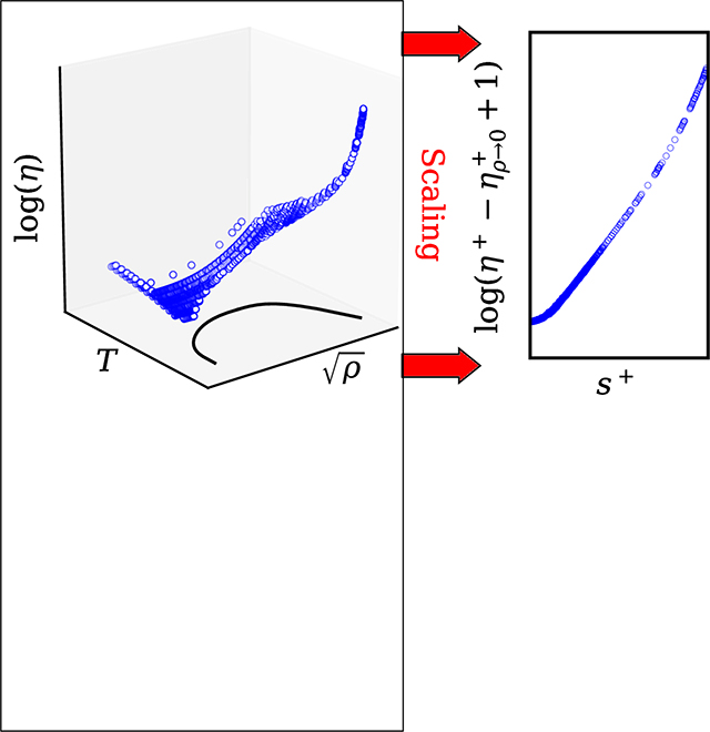
Graphical Abstract

1. Introduction

1.1. Background

The state-of-the-art for reference viscosity models (e.g., those of carbon dioxide,¹ n-butane,² ammonia³ to name but three recent examples) is based upon a very wide range of functional forms and a greater or lesser basis in theory. Having personally implemented nearly all the reference correlations from the last few decades,⁴ it became painfully clear that a new approach was needed with a strong theoretical basis and broadly applicable (but flexible enough) functional form. This works demonstrates that entropy scaling can move us in that direction, though perhaps not all the way.

There have been many attempts to express the transport properties of fluids in terms of thermodynamic properties, with more or less theoretical rigor. Some of them have at their heart a direct connection to the hard sphere,^5–10 and others consider some sort of free volume as their independent variable.¹¹ It is argued here that these historical approaches can all be reconciled through the residual entropy. The “available volume” (sometimes called the free volume) is directly related to residual properties, particularly the residual entropy. The lacunarity of the fluid (the amount of available volume) is directly related to the residual entropy,^12,13 and Mayer cluster theory also expresses a direct link between residual properties and the logarithm of the “available” volume.¹⁴

The first steps in the direction of entropy scaling came from the use of density scaling.^1,15–19 In density scaling, the supposition is that all properties can be expressed in terms of the independent variable ρ^γ/T, where the coefficient γ is a constant over the entire phase diagram. The parameter γ can be evaluated from either an equation of state or from fluctuations of the potential energy and the virial energy in a molecular simulation (e.g., see Eq. 9 of Ref. 20). Either route for its evaluation shows that γ is not a constant, but has both temperature and density dependence, and goes to zero at the critical point. Density scaling can therefore be thought of as a weak form of entropy scaling, though it has the clear benefit compared with entropy scaling that no equation of state is invoked to calculate the residual entropy (though the equation of state is still used to calculate the densities for a particular temperature, pressure measurement).

1.2. Entropy scaling and isomorph theory

Isomorph theory is an approximate theory describing that when the Pearson correlation between the time histories of the potential energy U of the ensemble and the virial energy W (W/V = p−Nk_BT/V) are strong, there are isomorphs in the phase diagram. Isomorphs are lines of constant reduced structure (iso: same, morph: morphology (structure)) along which certain properties are constant, among which are residual entropy and macroscopically-scaled viscosity $\tilde{\eta }$. According to the present understanding, the only pair potential for which isomorph theory holds exactly is the inverse-power-law potential V = ε(σ/r)ⁿ in which ε is the energy scale, σ is the length scale, and r is the distance between particles. This potential has the independent variable ρ^n/3/T, which describes the link to density scaling – if a fluid were to have a constant γ = n/3 (but it does not), then the expectation would be that $\eta /\left({\rho }_{\text{N}}^{2/3}\sqrt{m{k}_{\text{B}}T}\right)$ is a monovariate function of ρ^γ/T over the entire phase diagram.

The macroscopically-scaled viscosity²¹ is given by

$$\tilde{\eta }\equiv \frac{\eta }{{\rho }_{\text{N}}^{2/3}\sqrt{m{k}_{\text{B}}T}}$$ (1)

where η is the shear viscosity, ρ_N is the number density in particles per volume, m is the mass of one particle, k_B is Boltzmann’s constant, and T is the absolute temperature. The number density is obtained by multiplying the molar density (in mol/m³) by Avogadro’s number.²²

The residual entropy is defined by

$$s^{\text{r}}\left(T,{\rho }_{\text{N}}\right)\equiv s\left(T,{\rho }_{\text{N}}\right)-s^{(0)}\left(T,{\rho }_{\text{N}}\right)$$ (2)

where s^r is the residual entropy, s is the total entropy, and s⁽⁰⁾ is the ideal-gas entropy.

The variable

$$s^{+}\equiv -s^{\text{r}}/k_{\text{B}},$$ (3)

in which s^r is per particle, is defined, for conceptual understanding and brevity. The residual entropy can be conceptually understood as a measure of the structure of the fluid; the more positive s⁺ is (or negative s^r is), the more “structured” the fluid is. The residual entropy measures the change in the number of accessible microstates compared with the ideal-gas at the same temperature and density, and is therefore always negative.

In 1999, Rosenfeld²³ noted that for dilute gases of finite density, the macroscopically reduced transport properties are proportional to the residual entropy to the power of −2/3, based on a study of inverse power law potentials. An empirical scaling approach that satisfies the necessary behavior in the liquid phase²⁴ and the gas phase²³ is to multiply the macroscopically-reduced transport properties by the residual entropy to the power of 2/3, and use this scaling throughout the entire fluid domain, including the zero-density limit. This approach was first proposed in Ref. 25, and subsequently investigated in detail for the Lennard-Jones 12–6 fluid.²⁶ Thus the +-scaled viscosity is given by

$${\eta }^{+}\equiv \tilde{\eta }\times {\left(s^{+}\right)}^{2/3}$$ (4)

1.3. Residual Entropy

The residual entropy is defined by Eq. (2), and can be evaluated by a number of means. When an equation of state can be written in the form of the Helmholtz energy as a function of the temperature and density, the residual entropy can be obtained as a derivative of the residual Helmholtz energy. The residual energy term s⁺ can therefore alternatively be defined by

$$s^{+}=\frac{1}{k_{\text{B}}}{\left(\frac{\partial a^{\text{r}}}{\partial T}\right)}_{\rho }=T{\left(\frac{\partial {\alpha }^{\text{r}}}{\partial T}\right)}_{{\rho }_{\text{N}}}+{\alpha }^{\text{r}}$$ (5)

in which a^r is the residual Helmholtz energy per particle and α^r = a^r/(k_BT) is the reduced residual Helmholtz energy.

The van der Waals^27,28 (vdW) equation of state (EOS) is given by

$$p=\frac{RT}{v-b}-\frac{a}{v^2},$$ (6)

where R is the universal molar gas constant, v is the molar volume, b is the covolume, and a accounts for attraction. The first term on the right-hand-side (RT/(v − b)) is the repulsive term and the second term (a/v²) is the attractive term. For this EOS, the residual entropy is simply (see section 1 of the SI)

$$s_{\text{vdW}}^{+}=-\ln \left(1-\frac{1}{8}\frac{k_{\text{B}}{T}_{\text{crit},i}}{p_{\text{crit},i}}{\rho }_{\text{N}}\right).$$ (7)

In the case of the vdW EOS, only the repulsive part of the EOS contributes to the residual entropy because a has no temperature dependence. Although the vdW EOS does not yield quantitatively correct thermodynamic properties, the vdW EOS provides a simple understanding of the residual entropy: the residual entropy is controlled by repulsion. This link was also probed by Brańka and Heyes²⁹ for inverse-power-law potentials. Modification of the vdW equation of state to add more complicated (and accurate) temperature dependence to the attraction (Peng-Robinson, SRK, etc.) can also be used in this framework, as these modified EOS can be transformed to a form similar to that of the fundamental equation of state.³⁰ Their residual entropies have a very simple functional dependency on temperature and density (see the SI, section 1).

In general, any EOS that can be written in Helmholtz-energy-explicit form could be used to calculate the residual entropy from Eq. (5). A particularly popular family of these models is the panoply of SAFT models; these EOS have been successfully used to develop generalized empirical models for transport properties from entropy scaling by the group of Joachim Gross.^31–34 Similarly, the cubic-plus-association (CPA) model has been used in concert with entropy scaling to model the viscosity of hydrofluoroolefin (HFO) refrigerants and their mixtures.³⁵

The most accurate representation of the residual entropy is provided by multiparameter reference equations of state. The fundamental equations of state implemented in libraries such as REFPROP,³⁶ CoolProp⁴ and TREND³⁷ are of the form α^r = f(τ, δ), where τ = T_red/T and δ = ρ/ρ_red, and T_red and ρ_red are the reducing temperature and reducing density, respectively. The reducing temperature and density are, with only a few historical exceptions, equal to the respective values at the critical point. In order to orient the reader, contour plots of s⁺ in the T v. ρ and ln(p) v. T coordinates for the reference equation of state of propane from Lemmon et al.³⁸ are provided in Fig. 1.

Figure 1:

Contours of s⁺ for propane according to the EOS of Lemmon et al.³⁸ in the T-ρ and log(p)-T planes

1.4. Summary

In short, many of the existing theoretical approaches for modeling transport properties have at their heart a direct link to the residual entropy, which is perhaps not surprising, because isomorph theory defines a rigorous (albeit approximate) relationship between transport properties, when appropriately scaled, and the residual entropy.

The primary thrust of this paper is to investigate in detail the residual entropy scaling of propane and identify limitations in this approach.

The paper is structured as follows: Section 2 provides a description of the overall approach for correlation development, Section 3 discusses the zero-density limit, Section 4 describes the initial density contribution, Section 5 presents a detailed discussion of the scaling steps, and Section 6 provides a future outlook.

2. Correlation

Propane has long been considered as a reference fluid for various scaling approaches, especially extended corresponding states^39–42 due to its anomalous thermophysical properties, especially its triple point temperature, which is lower than any other member of the linear alkane family as a fraction of its critical temperature. The reduced triple point temperatures (divided by the critical point temperature), according to the default multiparameter equations of state in NIST REFPROP 10,³⁶ for the first five normal alkanes (methane: 0.48, ethane: 0.30, propane: 0.23, n-butane: 0.32, n-pentane: 0.31) show a clear minimum for propane.

In order to explain the thought process that has resulted in the model formulation proposed in this work, the fluid propane and its scaling of viscosity is discussed at some length. This fluid is characterized by an accurate reference fundamental equation of state³⁸ and a significant body of experimental measurements of viscosity.

2.1. Functional Form

In the conventional construction of empirical model formulations for the viscosity, the correlation is often written in the form

$$\eta ={\eta }_{{\rho }_{\text{N}}\to 0}(T)+{\eta }_{\text{init}}(T,\rho )+{\eta }_{\text{r}}(T,\rho )+\Delta {\eta }_{\text{crit}}(T,\rho )$$ (8)

in which ${\eta }_{{\rho }_{\text{N}}\to 0}$ is the dilute-gas contribution in the limit of zero density, η_init is the initial density contribution, η_r is the residual contribution, Δη_crit is the critical enhancement, T is the temperature, and ρ is the density (one of the molar density, mass density, or number density).

The critical enhancement term Δη_crit is relevant only in a very tiny region of the T, ρ plane around the critical point, and for all intents and purposes can be neglected for nearly all practical applications, as will be done here. Even when trying to extract the critical enhancement from measurements along near-critical isotherms, this exercise proves challenging.⁴³

In this work, the same basic functional form is considered, but all terms are transformed into the modified residual entropy scaled analog. These transformations result in terms that are related to their conventional counterparts, but are fundamentally different in their behavior. The functional form is then equal to

$${\eta }^{+}={\eta }_{{\rho }_{\text{N}}\to 0}^{+}(T)+{\eta }_{\text{init}}^{+}(T,\rho )+{\eta }_{\text{r}}^{+}(T,\rho )$$ (9)

2.2. Data

A sufficient amount of experimental viscosity data is available such that a reference viscosity correlation has been constructed,⁴³ and a number of previous correlations can be found in the literature for this fluid (see the description in section 1.1 of Ref. 43). In their work, Vogel and Herrmann⁴³ divided the experimental data into primary data (measurements that are believed to be reliable, highly accurate, and for which uncertainty estimates are available) and secondary data (not meeting the criteria to be primary data) and the same approach is followed in this work. The primary experimental data curated in the work of Vogel and Herrmann are provided in the supporting information in the units of the original publications for reproducibility. Other authors are recommended to follow the same protocol in order to avoid ambiguity about precisely which data were considered, what typographical errors were fixed (or introduced) and all the steps that were invoked to pre-process the experimental data.

Where densities were provided in the original dataset,⁵⁴ they were used directly, and otherwise, the equation of state was used to calculate the density from the given temperature and pressure pair, or temperature and vapor quality. Table 1 summarizes the primary data.

Table 1:

The primary data for propane as screened by Vogel and Herrmann.⁴³ For N_data, the ratio is that of the primary data points to the total number of data points in the dataset. The relative standard uncertainties Δη_s/η × 100 are as given in Vogel and Herrmann.⁴³ The values of s⁺ are as calculated from the EOS of Lemmon et al.³⁸ The complete set of data is in the SI in tabular form.

Year	Author	Ndata	Δηs/η × 100	T / K	p / MPa	s+
1959	Starling44	433/433	2.5	298.14 – 410.91	0.7 – 62.1	0.057 – 3.977
1960	Swift45	13/14	2.5	243.17 – 363.12	0.3 – 4.1	1.731 – 4.075
1964	Carmichael46	50/50	2.5	277.59 – 477.60	0.1 – 34.7	0.009 – 3.917
1966	Giddings47	73/78	2.5	277.59 – 377.57	0.7 – 55.2	0.065 – 4.045
1966	Huang48	30/30	2.5	173.19 – 273.15	6.9 – 34.5	3.609 – 6.210
1974	Strumpf49	5/5	2.5	310.92 – 310.92	3.2 – 7.2	2.848 – 2.963
1977	Kestin50	5/5	1.0	299.47 – 478.14	0.1 – 0.1	0.005 – 0.018
1978	Abe51	5/5	1.0	298.14 – 468.11	0.1 – 0.1	0.005 – 0.019
1979	Abe52	6/6	1.0	298.14 – 468.11	0.1 – 0.1	0.005 – 0.019
1982	Diller53	83/84	2.5	90.01 – 299.99	1.7 – 31.5	2.982 – 9.909
2011	Seibt54	181/212	0.5	273.18 – 423.10	0.1 – 29.8	0.010 – 2.633
2011	Wilhelm55	589/614	0.7	298.18 – 423.26	0.1 – 20.7	0.010 – 2.422
2016	Vogel56	70/70	0.3	297.24 – 625.80		0.002 – 0.023

The datasets from Starling⁴⁴ and Carmichael⁴⁶ represent data for which multiple measurements were carried out at each nominal state point. While Vogel and Herrmann averaged the replicate state points together,⁵⁷ all the data points were retained in this work. In addition, the low-density data of Vogel⁵⁸ re-evaluated in Ref. 43 were included as primary data. Temperatures reported on temperature scales prior to ITS-90 were converted to the ITS-90 temperature according to the supplement to the ITS-90 temperature scale,⁵⁹ and the scripts for these conversions are included in the supporting information.

3. Limit of Zero Density

In the limit of zero density, the interactions in the ensemble are reduced to pair-wise interactions. The interactions between gases are infrequent (compared with the liquid phase) and the motion is primarily ballistic.

The viscosity can be obtained from

$${\eta }_{{\rho }_{\text{N}}\to 0}=\frac{5}{16}{\left(\frac{m{k}_{\text{B}}T}{\pi }\right)}^{1/2}\frac{1}{{\sigma }^2{\mathrm{\Omega }}^{(2,2)*}}$$ (10)

where Ω^(2,2)* is the reduced collision integral obtained by integrating the possible approach trajectories of the particles, and σ is the length scale.

In practice, it is not possible to carry out experiments at zero density, and as a result, measurements at low density are extrapolated to zero density in order to provide experimental data for the dilute-gas contribution. Low-density measurements are usually carried out along nominal isotherms, potentially corrected back to the nominal temperature, and then extrapolated to zero density.

In recent years, very accurate ab initio calculations have been used to obtain dilute gas viscosity values for small rigid molecules.^60–73 The study of Hellmann et al.⁷¹ provides calculations for the dilute-gas transport properties of propane; this is one of the molecules with the largest number of atoms that has been studied to date. In addition, there are extrapolated values for the dilute-gas limit for propane available in the literature.⁴³

In the framework of modified residual entropy scaling,^26,74 it was shown that the zero-density limit of η⁺ from Eq. (4) takes the form

$${\eta }_{{\rho }_{\text{N}}\to 0}^{+}=\frac{{\eta }_{{\rho }_{\text{N}}\to 0}}{\sqrt{m{k}_{\text{B}}T}}{\mathfrak{B}}_2^{2/3}.$$ (11)

The term

$${\mathfrak{B}}_2\equiv \left(\frac{\text{d}\left(T{B}_2\right)}{\text{d}T}\right)=\left(T\left(\frac{\text{d}{B}_2}{\text{d}T}\right)+B_2\right)$$ (12)

is the zero-density limit of s⁺/ρ_N; B₂ is the second virial coefficient in a density expansion of the compressibility factor (i.e.,$p/\left({\rho }_{\text{N}}{k}_{\text{B}}T\right)=1+{\sum }_{m=2}^{\infty }{B}_m{\rho }_{\text{N}}^{m-1}$), and is given in terms of volume per molecule for dimensional consistency (i.e., not per mole). Please see Ref. 26 for a derivation of this result.

Thus, a model for ${\eta }_{\rho \to 0}^{+}$ is formed of two parts: one for the dilute-gas viscosity contribution ${\eta }_{{\rho }_{\text{N}}\to 0}$, and another for ${\mathfrak{B}}_2$. Combining the parts together, Fig. 2 presents the scaled dilute gas viscosity for propane. The following sections describe the contributions individually.

Figure 2:

Values of ${\eta }_{\rho \to 0}^{+}$ for propane from Eq. (11), combining Eq. (12) and the dilute-gas viscosity of Vogel and Herrmann.43 The dashed line corresponds to the “universal” high temperature limit of 0.27 (see Ref. 74)

3.1. Viscosity contribution

For ${\eta }_{\rho \to 0}/\sqrt{m{k}_{\text{B}}T}$ of propane, the correlation of Vogel and Herrmann⁴³ was used, in spite of its erroneous low- and high-temperature extrapolation behavior.⁷¹ A sensitive test for the proper behavior of the correlation is to consider the effective collisional cross-sectional area, proportional to $\sqrt{T}/{\eta }_{\rho \to 0}$. The current understanding is that this area should be infinite at zero temperature and smoothly approach zero at infinite temperature with no inflection points (always positive curvature), and be uniquely positive (never cross zero). In Fig. 3 are shown these areas calculated from the correlation of Vogel and Herrmann.⁴³ The correlation has an inflection point in the vicinity of 1250 K, although the propane molecule has already begun to thermally decompose at this temperature. Further constraints on the functional form can be obtained from the recent work on effective repulsive exponents of dilute gas thermophysical properties.⁷⁵

Figure 3:

Values of $\sqrt{T}/{\eta }_{\rho \to 0}$ for propane from the correlation of Vogel and Herrmann⁴³

3.2. Virial coefficient contribution

For a thermodynamic equation of state, the definition of B₂ comes from

$$B_2=\underset{{\rho }_{\text{N}}\to 0}{\lim }{\left(\frac{\partial {\alpha }^{\text{r}}}{\partial {\rho }_{\text{N}}}\right)}_T,$$ (13)

and B₂ and its temperature derivative can be obtained from the equation of state (see the supporting information of Ref. 26). For the equation of state of Lemmon et al.,³⁸ the EOS provides the virial coefficients as the terms of the equation of state with a density exponent of 1. Please see the SI for the details (section 4).

4. Initial Density

While ab initio calculations can provide zero-density-limit values for the viscosity, the low-density gas of finite density is less accessible to theory. It is accepted practice to consider a virial expansion of viscosity for very low densities in terms of the number density as (note the next term is not simply ${\eta }_{\rho \to 0}{B}_{\eta 2}{\rho }_{\text{N}}^2$; see Eq. 5.1 in Ref. 76)

$$\eta ={\eta }_{\rho \to 0}+{\eta }_{\rho \to 0}{B}_{\eta 1}{\rho }_{\text{N}}+\dots$$ (14)

where the second term on the right-hand-side is the initial density contribution of Eq. (8).

Rainwater-Friend theory^77,78 (originally developed based on the results for the Lennard-Jones fluid) gives a way to obtain an empirical correction at low densities. The term B_η1 can be obtained from a fit to the modified Rainwater-Friend theory.⁴³

$$B_{\eta 1}^{*}\equiv \frac{B_{\eta 1}}{{\sigma }^3}=\sum _{i=0}^6{b}_i{\left(T^{*}\right)}^{-i/4}+b_7{\left(T^{*}\right)}^{-2.5}+b_8{\left(T^{*}\right)}^{-5.5}$$ (15)

with the coefficients in Table 2 and T* defined by T* = T/(ε/k_B). The parameters σ and ε/k_B are empirical coefficients used to shift the initial density curve for the fluid to align with that of Lennard-Jones.

Table 2:

Coefficients for fit of Rainwater-Friend theory for the Lennard-Jones fluid from Vogel et al.⁷⁹

i	bi	i	bi
0	−19.572881	5	2491.6597
1	219.73999	6	−787.26086
2	−1015.3226	7	14.085455
3	2471.01251	8	−0.34664158
4	−3375.1717

If low-density experimental viscosity data are available along nominal isotherms, a quadratic function of the form

$$\eta =a+b{\rho }_{\text{N}}+c{\rho }_{\text{N}}^2$$ (16)

can be fit to the viscosity data along it in terms of the number density ρ_N. The initial viscosity exponent B_η1 is then obtained from b/a as a consequence of the definition of B_η1

$$B_{\eta 1}=\frac{1}{{\eta }_{\rho \to 0}}\times \left(\underset{{\rho }_{\text{N}}\to 0}{\lim }{\left(\frac{\partial \eta }{\partial {\rho }_{\text{N}}}\right)}_T\right)$$ (17)

Figure 4 shows the initial density terms calculated from Rainwater-Friend theory and the experimental data. In the case of Vogel,⁵⁸ the data were taken from the re-evaluated data,⁴³ and then mapped back onto the nominal isotherms identified in Vogel and Herrmann⁴³ following the same approach in Vogel and Herrmann;⁴³ the data mapped onto isotherms are in the SI (Section 3.1). The data for Wilhelm and Vogel⁸⁰ and Seibt et al.⁵⁴ were processed in a simple fashion: Eq. (16) was fit to the data for s⁺ < 0.1 along nominal isotherms in order to extract B_η1.

Figure 4:

The first viscosity virial coefficient (upper) and the equivalent term for the residual entropy formulation of the virial expansion (lower) for propane. The solid curve is obtained from Rainwater-Friend theory with the Lennard-Jones coefficients from Ref.⁵⁸ and the values of ε/k_B = 260 K and σ = 0.49154 × 10⁻⁹ m. The markers correspond to the considered datasets from Wilhelm,⁸⁰ Seibt⁵⁴ and the re-evaluated data from Vogel⁵⁸ in Ref. 43.

If instead of an expansion in number density, an expansion in s⁺ is constructed, a similar form is obtained:

$${\eta }^{+}={\eta }_{\rho \to 0}^{+}+{\eta }_{\rho \to 0}^{+}{B}_{\eta 1}^{+}{s}^{+}+\dots$$ (18)

After some mathematics (see the SI, Section 3.3), it can be shown that the viscosity virial coefficient in a s⁺ expansion is related to that of the density expansion by

$$B_{\eta 1}^{+}\equiv \underset{{\rho }_{\text{N}}\to 0}{\lim }\frac{1}{{\eta }_{\rho \to 0}^{+}}{\left(\frac{\partial {\eta }^{+}}{\partial s^{+}}\right)}_T=\frac{1}{{\mathfrak{B}}_2}\left[\frac{1}{3}\frac{{\mathfrak{B}}_3}{{\mathfrak{B}}_2}+B_{\eta 1}\right]$$ (19)

in which

$${\mathfrak{B}}_3\equiv B_3+T\left(\frac{\text{d}{B}_3}{dT}\right).$$ (20)

and B₃ is the third virial coefficient. The values of B₃ are rarely known very accurately, aside for a few special cases (e.g., the Lennard-Jones fluid,⁸¹ helium-4,⁸² nitrogen,⁶⁵ argon,⁸³ krypton,⁸⁴ CO₂,⁸⁵ two-center Lennard-Jones dimer with embedded quadrupole⁸⁶); many of the multiparameter equations of state yield erroneous virial coefficients above B₂. But even the second virial coefficient B₂ causes trouble: for many fluids the paucity of data in the gas phase means that the EOS values for B₂ are guided by intuition rather than data.

One of the few cases in which values of $B_{\eta 1}^{+}$ can be calculated directly is the Lennard-Jones fluid. In this case, all contributions to Eq. (19) can be reliably calculated, providing guidance on the correct shape of the curve for other fluids that can be treated in analogy to the Lennard-Jones fluid. In Fig. 5 are shown the values of $B_{\eta 1}^{+}$ calculated from Eq. (19), $B_{\eta 1}^{*}$ obtained from Eq. (15), and $B_{\eta 1}^{*}/{\mathfrak{B}}_2^{*}$. The values of ${\mathfrak{B}}_2^{*}$ are always positive,⁷⁴ and therefore, the zeros of $B_{\eta 1}^{*}$ will also be zeros of $B_{\eta 1}^{*}/{\mathfrak{B}}_2^{*}$. The most important conclusion of Fig. 5 is that $B_{\eta }^{+}$ is approximately equal to $B_{\eta 1}^{*}/{\mathfrak{B}}_2^{*}$. The contribution $B_{\eta 1}^{*}/{\mathfrak{B}}_2^{*}$ dominates that from ${\mathfrak{B}}_3^{*}/\left({\mathfrak{B}}_2^{*}\right)$², therefore, the accuracy of the third virial coefficients does not pose a major problem for evaluation of $B_{\eta 1}^{+}$. While Fig. 4 suggests that there is a linear relationship between B_η1 and T, Fig. 5 shows that for at least the Lennard-Jones fluid, that linear relationship only holds for part of the temperature range.

Figure 5:

Values of $B_{\eta 1}^{*}$ from Rainwater-Friend theory,⁷⁸ $B_{\eta 1}^{*}/{\mathfrak{B}}_2^{*}$ (with quasi-exact $B_2^{*}$ from the formulation reported in Sadus,^87,88 originally from Jones⁸⁹), and B⁺ from Eq. (19) (with interpolated values of ${\mathfrak{B}}_3^{*}$ from Ref. 81). Points are connected with straight line segments to guide the eye.

The contribution from the initial density term is relatively small. Figure 6 shows the relative contributions to η⁺ from the initial density term ${\eta }_1^{+}={\eta }_{{\rho }_{\text{N}}\to 0}^{+}{B}_{\eta 1}^{+}{s}^{+}$ and the dilute-gas term (Eq. (10)). The maximum absolute relative contribution from the initial density term is approximately 8%. In the liquid phase, the contribution is approximately the same relative amount in the opposite direction, a consequence of temperatures for which Eq. (15) is negative.

Figure 6:

Relative contributions to η⁺ from the dilute (Eq. (11)) and initial density contributions (Eq. (18)). Each dot corresponds to one data point.

5. Scaling Analysis

The primary experimental data for propane are plotted in Fig. 7 as a function of temperature and molar density. The data provide a good coverage of the $T-\sqrt{\rho }$ plane, and η varies over approximately three orders of magnitude.

Figure 7:

Overview of the primary viscosity data for propane identified by Vogel and Herrmann.⁴³ The data points, shown in the T, ρ plane, are colored by the base 10 logarithm of the viscosity

The introduction of residual entropy scaling transforms the data entirely. To begin, macroscopic scaling is applied to the experimental data according to Eq. (1) and $\tilde{\eta }$ is plotted as a function of s+. This scaling, shown in Fig. 8, demonstrates a behavior that is to be expected for most fluids: the scaling approach turns the viscosity data (formerly a function of temperature and density; see Fig. 7) into a nearly-monovariate function of s⁺. The location of the minima of $\tilde{\eta }$ represents, according to our work,⁹⁰ the crossover between gas-like and liquid-like behavior. Furthermore, the value $\left(s_{\text{crit}}^{+}+s_{\text{trip}}^{+}\right)/2$ appears to represent the changeover between two different regimes in the dynamics; for $s_{\text{crit}}^{+}<s^{+}<(s_{\text{crit}}^{+}+s_{\text{trip}}^{+})/2$ the relationship between $\log (\tilde{\eta })$ and s⁺ is nearly linear, a similar result also seen for the Lennard-Jones fluid.²⁶

Figure 8:

Overview of the macroscopically-scaled primary viscosity data for propane identified by Vogel and Herrmann.⁴³ A detailed view of the critical region (indicated by the box) is in Fig. 9

While not readily visible in Fig. 8, there remains a small departure from monovariate scaling in the extended region around the critical point and can be seen in Fig. 9, characterized by its proximity to the critical point. This deviation is not a critical enhancement, rather it is a reduction in $\tilde{\eta }$ relative to the high-temperature limit caused by breakdown of isomorph theory. High-temperature physics are dominated by repulsion, and as temperatures increase, isomorph theory becomes a better and better approximation to the actual physics.

Figure 9:

The macroscopically-scaled primary viscosity data^{44–47,54,80} in the critical region.

One of the unfortunate “features” of macroscopic scaling is the divergence of $\tilde{\eta }$ at zero density caused by the term $1/{\rho }_{\text{N}}^{2/3}$. It is decidedly inconvenient to develop correlations of divergent data, so alternative approaches that empirically “fix” this divergence have been proposed,^{31–34,91,92} but these corrections (the Novak scaling approach) introduce a new problem. A necessary condition for the application of isomorph theory is that the viscosity be non-dimensionalized by the appropriate dimensional scales (length: ${\rho }_{\text{N}}^{-1/3}$, energy: k_BT, time: ${\rho }_{\text{N}}^{-1/3}\sqrt{m/\left(k_{\text{B}}T\right)})$,²¹ yielding a scaling term of ${\rho }_{\text{N}}^{2/3}\sqrt{m{k}_{\text{B}}T}$ for viscosity (base SI units of viscosity are kg m⁻¹ s⁻¹). The zero-density-limit viscosity has no density dependence and has the length scale of σ. The use of the resulting viscosity scaling parameter ${\sigma }^2\sqrt{m{k}_{\text{B}}T}$ in place of ${\rho }_{\text{N}}^{2/3}\sqrt{m{k}_{\text{B}}T}$ results in a destruction of the monovariate scaling in the liquid phase for small molecules (e.g., argon²⁵). For larger molecules, use of the microscopic length scale σ in place of ${\rho }_{\text{N}}^{-1/3}$ has a relatively modest impact and quite accurate transport models can be developed.

An approach which a) repairs the divergence at zero density b) uses the correct length scale and c) retains the nearly monovariate scaling in the liquid phase is modified residual entropy scaling. This approach was first investigated in detail for the Lennard-Jones model fluid,²⁶ though it had been introduced without investigation in Ref. 25. This scaling approach has a well-formed dilute-gas limit without any divergence and does not impact the residual entropy scaling in the liquid phase. Therefore, Fig. 10 shows the primary data according to residual entropy scaling.

Figure 10:

Overview of the +-scaled primary viscosity data for propane identified by Vogel and Herrmann.⁴³ A detailed view of the gas phase is in Fig. 11.

In the low (but finite) density gas, the values of η⁺ are no longer a monovariate function of s⁺, but they have a well-characterized limit at zero density (see Section 3). Figure 11 shows the scaled viscosity data at relatively low densities.

Figure 11:

Scaled data at low density. The lines (colored with the same scale) have slopes obtained from the initial density term in Eq. (19), and are shown to highlight that the initial density term is coherent with the low-density data.

Combining all these approaches, Fig. 12 shows the residual contribution to viscosity (in +-scaled coordinates), obtained by subtracting off the dilute-gas contribution ${\eta }_{\rho \to 0}^{+}$. The offset value of 1 is added to ensure that the data can still be plotted in semilog coordinates. The offset factor could be set to any desired value greater than zero. The deviation from monovariability in the gaseous region is still present.

Figure 12:

Overview of the +-scaled primary viscosity data for propane identified by Vogel and Herrmann.⁴³ The solid line is the Arrhenius curve, the dashed curve is the gas curve, and the dashed-dotted curve is the super-Arrhenius curve.

In this figure, the phase diagram is roughly divided into three portions. In the gaseous region, here containing the dilute-gas limit to the extended critical region, the physics is complicated. In this region the motion is neither ballistic (as in the case of the dilute gas) nor correlating (in the isomorph theory sense). For larger values of s⁺ (but not too large), an “Arrhenius” region can be identified in which the ordinate demonstrates an exponential dependence on s⁺ (linear in semilog coordinates). At even higher values of s⁺, a super-Arrhenius region can be identified in which the ordinate increases much faster than exponential as s⁺ increases. It is true that there is not a one-to-one relationship between the present definition of Arrhenius and super-Arrhenius behavior and the conventional ones; the conventional definitions of these terms are based on the pressure as the independent variable.^93,94 The present use of the term Arrhenius is simply a convenient lexicon, and useful for mapping the behavior of real fluids onto one another.

One of the primary goals of this work is to demonstrate that entropy scaling can be used to construct correlations approaching reference quality with minimal empiricism. Therefore, the empirical model developed here is not the most accurate model possible (a target for future work), rather it demonstrates the power of this scaling approach in general. The heart of the correlation is the linear Arrhenius region, upon which all the other parts build. The scaled residual viscosity is defined by

$$\mathrm{\Upsilon }={\eta }^{+}-{\eta }_{\rho \to 0}^{+}+1$$ (21)

The variable Υ is defined to make the mathematics more concise.

To begin, a curve fit to the data in $s_1^{+}<s^{+}<s_2^{+}$ results in the line

$$\ln \left({\mathrm{\Upsilon }}_{\text{Ar}}\right)=m_{\text{Ar}}{s}^{+}+b_{\text{Ar}}.$$ (22)

with the coefficients m_Ar = 0.63392108, b_Ar = −0.5339991, and the Arrhenius “window” defined by the values of $s_1^{+}=2$ and $s_2^{+}=5.4$.

The gas region is obtained by the cubic curve

$$\ln \left({\mathrm{\Upsilon }}_{\text{g}}\right)=\sum _{i=0}^3{a}_i{\left(s^{+}\right)}^i$$ (23)

for the domain $0<s^{+}<s_1^{+}$, with four constraints:

1. the value of Υ_g is 1 at s⁺ = 0

2. the initial slope d ln Υ_g/ds⁺ at s⁺ = 0 is determined by the initial density term in Section 4

3. at $s^{+}=s_1^{+}$, the value is $m_{\text{Ar}}{s}_1^{+}+b_{\text{Ar}}$

4. the slope d ln Υ_g/ds⁺ at $s^{+}=s_1^{+}$ equals m_Ar.

The gas portion is therefore modeled with no additional adjustable parameters, simply a smooth transition from the Arrhenius region to the zero-density limit. The first constraint yields a₀ = 0. The second constraint yields $a_1={\eta }_{{\rho }_{\text{N}}\to 0}^{+}{B}_{\eta 1}^{+}$, and the remaining (temperature-dependent) coefficients are obtained by solving the 2×2 linear system with the use of Cramer’s rule for a₂ and a₃ to obtain

$$a_2(T)=\frac{s_1^{+}\left(2m_{\text{Ar}}-2a_1(T)\right)+3b_{\text{Ar}}}{{\left(s_1^{+}\right)}^2}$$ (24)

$$a_3(T)=\frac{s_1^{+}\left(a_1(T)-m_{\text{Ar}}\right)-2b_{\text{Ar}}}{{\left(s_1^{+}\right)}^3}$$ (25)

In the super-Arrhenius region $\left(s^{+}>s_2^{+}\right)$, the approach is similar, but the functional relationship employed is somewhat different. Inspired by noting that ln(ln(Υ_SA)) is approximately a linear function of ln(s⁺) in the approach to the melting line, the “Super-Arrhenius” region was correlated as

$$\ln \left(\ln \left({\mathrm{\Upsilon }}_{\text{SA}}\right)\right)=\sum _{i=0}^2{c}_i{\left(\ln \left(s^{+}\right)\right)}^i.$$ (26)

Two constraints come from the Arrhenius region:

1. At $s_2^{+}$, the value of ln(Υ_SA) is equal to $m_{\text{Ar}}{s}_2^{+}+b_{\text{Ar}}$

2. At $s_2^{+}$, the slope d ln Υ_SA/ds⁺ is that of the Arrhenius region (m_Ar), with the relationship

$$\left(\frac{\text{d}\ln \left(\ln \left({\mathrm{\Upsilon }}_{\text{SA}}\right)\right)}{\text{d}\ln \left(s^{+}\right)}\right)=\left(\frac{\text{d}\ln \left({\mathrm{\Upsilon }}_{\text{SA}}\right)}{\text{d}{s}^{+}}\right)\frac{s^{+}}{\ln \left({\mathrm{\Upsilon }}_{\text{SA}}\right)}$$ (27)

One adjustable parameter remains and a single datapoint at $\left(s_3^{+},{\mathrm{\Upsilon }}_3\right)$ is the third value constraint on the super-Arrhenius curve, fully defining the quadratic. The 3×3 system of equations to be solved for the coefficients c_i is therefore:

$$\left[\begin{array}{ccc}1& \ln \left(s_2^{+}\right)& {\ln }^2\left(s_2^{+}\right)\\ 0& 1& 2\ln \left(s_2^{+}\right)\\ 1& \ln \left(s_3^{+}\right)& {\ln }^2\left(s_3^{+}\right)\end{array}\right]\left[\begin{array}{c}{c}_0\\ c_1\\ c_2\end{array}\right]=\left[\frac{\begin{array}{c}\ln \left(m_{\text{Ar}}{s}_2^{+}+b_{\text{Ar}}\right)\\ m_{\text{Ar}}{s}_2^{+}\end{array}}{\begin{array}{l}{m}_{\text{Ar}}{s}_2^{+}+b_{\text{Ar}}\\ \ln \left(\ln \left({\mathrm{\Upsilon }}_3\right)\right)\end{array}}\right]$$ (28)

for which the coefficients c₀ = 0.316991, c₁ = −0.302498, c₂ = 0.440977 are obtained, of which only one should be considered an adjustable parameter.

In summary, the correlation is defined piecewise, with continuous values and derivative ensured between sections so that no smoothing across segment boundaries is required. The full implementation of the correlation is defined by

$$\ln (\mathrm{\Upsilon })=\{\begin{array}{ll}{\mathrm{\Upsilon }}_{\text{g}}& s^{+}<s_1^{+}\\ {\mathrm{\Upsilon }}_{\text{Ar}}& s_1^{+}\le s^{+}\le s_2^{+}\\ {\mathrm{\Upsilon }}_{\text{SA}}& s^{+}>s_2^{+}\end{array}$$ (29)

with the contributions from Eq. (23), Eq. (22), and Eq. (26), respectively. A complete Python implementation of the correlation is in Fig. 14. The extrapolation behavior of the correlation is shown in Fig. 13, demonstrating a smoothly varying behavior up to non-physical densities far beyond the melting line. This smooth extrapolation behavior is partially ensured by the smooth function in Eq. (26), and partially by the well-behaved EOS.

Figure 14:

A Python 3.x implementation of the proposed correlation. The thermo module is in the supporting information and includes the complete evaluation of s⁺, ${\mathfrak{B}}_2$, and ${\mathfrak{B}}_3$ for a given temperature and density.

Figure 13:

Extrapolation test of the correlation, showing smooth extrapolation up to 1000 K and a density approximately three times the density of the liquid at the triple-point. The solid white lines indicate interpolated contours of iso-viscosity up to 10¹⁰ Pa s. The thick red line indicates the melting line from Ref. 95, valid up to 1.1 × 10⁹ Pa, and extrapolated to 10¹⁰ Pa.

Deviations between the correlation and the experimental data are shown in Fig. 15. The deviations are colored by the values of $c_v^{\text{r}}/k_{\text{B}}$ because $c_v^{\text{r}}/k_{\text{B}}$ (to first order) should be constant along the curve of constant s⁺ when isomorph theory should apply.⁹⁶ The error bands indicated in the figure are the central 68% and 95% percentiles of the error histogram. The expanded uncertainty (k=2) of this correlation could be defined to be −4.81% to 4.61%, or more conservatively, ±4.9%. The average absolute relative error is 1.38%, a factor of more than three smaller than a previous entropy scaling approach³⁴ (the included datasets differ, and are not documented in Ref. 34). In the vicinity of $s_{\text{crit}}^{+}$, the deviations are large, but are strongly correlated with the value of $c_v^{\text{r}}$, suggesting that isomorph theory is no longer applicable in this part of the phase diagram.²⁶ Aside from the measurements^54,55 with ascribed standard uncertainties less than 1%, the measurements are otherwise mostly reproduced within twice the ascribed standard uncertainty with three adjustable parameters.

Figure 15:

Deviations between the model predictions of this work and the experimental values. The dashed-dotted horizontal lines indicate the central 68% percentiles and the horizontal dashed lines the central 95% percentiles.

The functional form selected is intentionally simplistic for demonstration purposes, the “wiggles” in the deviations (but with less significant scatter orthogonal to the wiggles) indicate that a functional form with more flexibility would offer a better fit to the data, while still being a monovariate function of s⁺. A variety of functional forms (e.g., rational polynomials, Chebyshev expansions⁹⁷) have been used to obtain a more flexible function to fit ln(Υ(s⁺)) and they are able to tighten the 95% confidence interval by approximately 1% in deviation at each end, and fit all the data for s⁺ > 4 within 2.5%, but the critical region bump remains.

The present reference viscosity model for propane is that of Vogel and Herrmann,⁴³ and Fig. 16 shows the deviations between the primary datasets and the implementation of this model from NIST REFPROP 10.³⁶ The overall statistics are undeniably superior with the model of Vogel and Herrmann⁴³ as compared to the present model, but the number of adjustable parameters is reduced by roughly 30 compared with Vogel and Herrmann. This accounting includes coefficients and exponents; there is no unambiguous definition of what should be considered an “adjustable” parameter. The reduction in the number of parameters significantly reduces the likelihood of over-fitting of the model.

Figure 16:

Deviations between the correlation of Vogel and Herrmann⁴³ and the experimental primary data values. See Fig. 15 for other formatting notes.

Invocation of the equation of state to evaluate s⁺ introduces a new source of uncertainty in the viscosity formulation. As a demonstration of the stability of this method to changes in the thermodynamic model, the equation of state was switched from Lemmon et al.³⁸ to Bücker et al.,⁹⁸ an equation of state that was developed based on n-butane and isobutane, and then parameters were optimized for propane. The deviation plot for the correlation, which was otherwise unchanged, is shown in Fig. 17. Except for at very high densities (large s⁺), the differences are difficult to see in the deviation plot, and the statistics for goodness-of-fit are similar.

Figure 17:

Deviations between the model predictions from this work and the experimental values with the thermodynamic model from Bücker et al.⁹⁸ See Fig. 15 for other formatting notes.

6. Outlook

Propane was studied in this work because it is well measured, has a high-quality equation of state, and represents intermediate behavior in the framework of entropy scaling.

In order to set the table for further studies, scaling results for other fluids are presented here in order to cover the range of behaviors to be expected. Here the data for propane are overlaid with the similarly scaled data for water and the Lennard-Jones fluid. Between these three fluids, they capture most of the qualitative behavior to be expected for real fluids.

For the Lennard-Jones fluid, a value of ${\eta }_{\rho \to 0}^{+}$ of 0.27 was assumed for all temperatures, and the correlation for the residual viscosity from Ref. 26 was used. This yields the correlation

$${\eta }^{+}=\exp \left(\sum _{i=1}^4{c}_i{\left(s^{+}\right)}^i\right)+0.27-1$$ (30)

with c₁ = 0.125364, c₂ = 0.220795, c₃ = −0.0313726, and c₄ = 0.00313907. For ordinary water, the data collection described in Ref. 25 was used, along with the equation of state of Wagner and Pruß⁹⁹ for s⁺.

Figure 18 shows the data overlaid. There are some important qualitative differences between the fluids. The first salient difference has to do with the convexity of the relationship between η⁺ and s⁺. In the case of the Lennard-Jones fluid, the curvature (that given by d² log(η⁺)/d(s⁺)²) is always positive, whereas in the case of propane, the curvature is positive at low and high values of s⁺, and has negative curvature otherwise.

Figure 18:

Scaled viscosity for the Lennard-Jones fluid, propane, and ordinary water

Water has a radically different behavior. Overall, the scaling tends to be much less monovariate, especially in the gaseous region and at very compressed states, where the presence of transitory hydrogen-bonding-networks destroys the correlating nature of the fluid. In spite of this, in a very qualitative sense, water is characterized by values of η⁺ that increase much slower with s⁺ than the other two fluids at relatively low values of s⁺, but increase much more rapidly in the liquid phase. These confounding features of water make it currently inaccessible to high-accuracy transport property modeling with entropy scaling, though this current state of affairs may not persist with future theoretical advances.

7. Conclusion

In this work it is shown that with the appropriate variable transformations it is possible to develop a very accurate viscosity correlation for propane from entropy scaling. This formulation is much simpler than existing approaches, has a solid theoretical basis, and very reliable extrapolation. At the dilute-gas limit, the appropriate behavior is guaranteed by the highly accurate ab initio calculations, and the higher-order terms in the liquid region are handled as a standard polynomial fitting problem.

In summary, this approach for developing transport property correlations has the advantages that it:

• Has only one independent variable (the residual entropy) in the dense phase as opposed to the temperature and density in conventional approaches.

• Has a theoretical basis coming from isomorph theory, which provides information about when this approach should be expected to work (or not).

• Requires no advanced fitting techniques to develop the model. Standard numerical tools can be used, and simple functional forms can be used.

• The simplicity of the functional form allows for straightforward analysis of the extrapolation behavior of the transport correlation (e.g, location of local extrema, roots, etc.). Potential issues in the extrapolation behavior of the equation of state remains a problem, as they do for conventional approaches.

On the other hand, some challenges of this new approach are that

• The equation of state itself is now invoked directly in the transport property model. As a result, changes to the equation of state might require a refitting of the transport property correlation, but this is also true for conventional correlations, where density is usually obtained from the equation of state rather than from the measurement itself.

• In the intermediate region in s⁺ isomorph theory breaks down, and an empirical correction term is needed. More detailed study of this region is needed in order to hopefully arrive at a theoretically sound approach for the isomorph theory correction.

• Equations of state that provide poor estimations of residual entropy are not suitable for development of transport property models from entropy scaling. Furthermore, novel analysis techniques need to be developed to better ascertain the uncertainty in residual properties in general because they are not measureable quantities. Some progress has been made in this direction from the quantification of equation of state statistical uncertainty.^100,101

References

- (1).Laesecke A; Muzny CD Reference Correlation for the Viscosity of Carbon Dioxide. J. Phys. Chem. Ref. Data 2017, 46, 013107, DOI: 10.1063/1.4977429. [DOI] [PMC free article] [PubMed] [Google Scholar]
- (2).Herrmann S; Vogel E New Formulation for the Viscosity of n-Butane. J. Phys. Chem. Ref. Data 2018, 47, 013104, DOI: 10.1063/1.5020802. [DOI] [Google Scholar]
- (3).Monogenidou SA; Assael MJ; Huber ML Reference Correlation for the Viscosity of Ammonia from the Triple Point to 725 K and up to 50 MPa. J. Phys. Chem. Ref. Data 2018, 47, 023102, DOI: 10.1063/1.5036724. [DOI] [PMC free article] [PubMed] [Google Scholar]
- (4).Bell IH; Wronski J; Quoilin S; Lemort V Pure and Pseudo-pure Fluid Thermophysical Property Evaluation and the Open-Source Thermophysical Property Library CoolProp. Ind. Eng. Chem. Res 2014, 53, 2498–2508, DOI: 10.1021/ie4033999. [DOI] [PMC free article] [PubMed] [Google Scholar]
- (5).Assael M; Dymond J; Papadaki M; Patterson P Correlation and prediction of dense fluid transport coefficients. Fluid Phase Equilib 1992, 75, 245–255, DOI: 10.1016/0378-3812(92)87021-e. [DOI] [Google Scholar]
- (6).Assael MJ; Dymond JH; Papadaki M; Patterson PM Correlation and prediction of dense fluid transport coefficients. III. n-alkane mixtures. Int. J. Thermophys 1992, 13, 659–669, DOI: 10.1007/bf00501947. [DOI] [Google Scholar]
- (7).Assael MJ; Dymond JH; Patterson PM Correlation and prediction of dense fluid transport coefficients. IV. A note on diffusion. Int. J. Thermophys 1992, 13, 729–733, DOI: 10.1007/bf00501953. [DOI] [Google Scholar]
- (8).Assael MJ; Dymond JH; Patterson PM Correlation and prediction of dense fluid transport coefficients. V. Aromatic hydrocarbons. Int. J. Thermophys 1992, 13, 895–905, DOI: 10.1007/bf00503914. [DOI] [Google Scholar]
- (9).Vesovic V; Wakeham WA The prediction of the viscosity of dense gas mixtures. Int. J. Thermophys 1989, 10, 125–132, DOI: 10.1007/bf00500713. [DOI] [Google Scholar]
- (10).Vesovic V; Wakeham W Prediction of the viscosity of fluid mixtures over wide ranges of temperature and pressure. Chem. Eng. Sci 1989, 44, 2181–2189, DOI: 10.1016/0009-2509(89)85152-8. [DOI] [Google Scholar]
- (11).Hildebrand JH Motions of Molecules in Liquids: Viscosity and Diffusivity. Science 1971, 174, 490–493, DOI: 10.1126/science.174.4008.490. [DOI] [PubMed] [Google Scholar]
- (12).Detmar E; Nezhad SY; Deiters UK Determination of the Residual Entropy of Simple Mixtures by Monte Carlo Simulation. Langmuir 2017, 33, 11603–11610, DOI: 10.1021/acs.langmuir.7b02000. [DOI] [PubMed] [Google Scholar]
- (13).Nezhad SY; Deiters UK Estimation of the entropy of fluids with Monte Carlo computer simulation. Mol. Phys 2016, 115, 1074–1085, DOI: 10.1080/00268976.2016.1238523. [DOI] [Google Scholar]
- (14).Woodcock LV Percolation transitions in the hard-sphere fluid. AIChE Journal 2011, 58, 1610–1618, DOI: 10.1002/aic.12666. [DOI] [Google Scholar]
- (15).Galliero G; Boned C; Fernández J Scaling of the viscosity of the Lennard-Jones chain fluid model, argon, and some normal alkanes. J. Chem. Phys 2011, 134, 064505, DOI: 10.1063/1.3553262. [DOI] [PubMed] [Google Scholar]
- (16).Ingebrigtsen TS; Schrøder TB; Dyre JC What Is a Simple Liquid? Phys. Rev. X 2012, 2, 011011, DOI: 10.1103/physrevx.2.011011. [DOI] [Google Scholar]
- (17).Dyre JC Isomorphs, hidden scale invariance, and quasiuniversality. Phys. Rev. E 2013, 88, 042139, DOI: 10.1103/physreve.88.042139. [DOI] [PubMed] [Google Scholar]
- (18).Ingebrigtsen TS; Schrøder TB; Dyre JC Isomorphs in Model Molecular Liquids. J. Phys. Chem. B 2012, 116, 1018–1034, DOI: 10.1021/jp2077402. [DOI] [PMC free article] [PubMed] [Google Scholar]
- (19).López ER; Pensado AS; Comuñas MJP; Pádua AAH; Fernández J; Harris KR Density scaling of the transport properties of molecular and ionic liquids. J. Chem. Phys 2011, 134, 144507, DOI: 10.1063/1.3575184. [DOI] [PubMed] [Google Scholar]
- (20).Schrøder TB; Gnan N; Pedersen UR; Bailey NP; Dyre JC Pressure-energy correlations in liquids. V. Isomorphs in generalized Lennard-Jones systems. J. Chem. Phys 2011, 134, 164505, DOI: 10.1063/1.3582900. [DOI] [PubMed] [Google Scholar]
- (21).Dyre JC Simple liquids’ quasiuniversality and the hard-sphere paradigm. J. Phys.: Condens. Matter 2016, 28, 323001, DOI: 10.1088/0953-8984/28/32/323001. [DOI] [PubMed] [Google Scholar]
- (22).Mohr PJ; Newell DB; Taylor BN; Tiesinga E Data and analysis for the CODATA 2017 special fundamental constants adjustment. Metrologia 2018, 55, 125–146, DOI: 10.1088/1681-7575/aa99bc. [DOI] [Google Scholar]
- (23).Rosenfeld Y A quasi-universal scaling law for atomic transport in simple fluids. J. Phys.: Condens. Matter 1999, 11, 5415–5427, DOI: 10.1088/0953-8984/11/28/303. [DOI] [Google Scholar]
- (24).Rosenfeld Y Relation between the transport coefficients and the internal entropy of simple systems. Phys. Rev. A 1977, 15, 2545–2549, DOI: 10.1103/PhysRevA.15.2545. [DOI] [Google Scholar]
- (25).Bell IH Probing the link between residual entropy and viscosity of molecular fluids and model potentials. Proc. Natl. Acad. Sci. U.S.A 2019, 116, 4070–4079, DOI: 10.1073/pnas.1815943116. [DOI] [PMC free article] [PubMed] [Google Scholar]
- (26).Bell IH; Messerly R; Thol M; Costigliola L; Dyre J Modified Entropy Scaling of the Transport Properties of the Lennard-Jones Fluid. J. Phys. Chem. B 2019, 123, 6345–6363, DOI: 10.1021/acs.jpcb.9b05808. [DOI] [PMC free article] [PubMed] [Google Scholar]
- (27).van der Waals JD Over de Continuiteit van den Gas- en Vloeistoftoestand. Ph.D. thesis, University of Leiden, 1873. [Google Scholar]
- (28).Kontogeorgis GM; Privat R; Jaubert J-N Taking Another Look at the van der Waals Equation of State–Almost 150 Years Later. J. Chem. Eng. Data 2019, DOI: 10.1021/acs.jced.9b00264. [DOI] [Google Scholar]
- (29).Brańka AC; Pieprzyk S; Heyes DM Thermodynamic curvature of soft-sphere fluids and solids. Phys. Rev. E 2018, 97, 022119, DOI: 10.1103/physreve.97.022119. [DOI] [PubMed] [Google Scholar]
- (30).Bell IH; Jäger A Helmholtz Energy Transformations of Common Cubic Equations of State for Use with Pure Fluids and Mixtures. J. Res. Nat. Inst. Stand. Technol 2016, 121, 238, DOI: 10.6028/jres.121.011. [DOI] [PMC free article] [PubMed] [Google Scholar]
- (31).Hopp M; Gross J Thermal Conductivity of Real Substances from Excess Entropy Scaling Using PCP-SAFT. Ind. Eng. Chem. Res 2017, 56, 4527–4538, DOI: 10.1021/acs.iecr.6b04289. [DOI] [Google Scholar]
- (32).Hopp M; Mele J; Gross J Self-Diffusion Coefficients from Entropy Scaling using the PCP-SAFT equation of state. Ind. Eng. Chem. Res 2018, DOI: 10.1021/acs.iecr.8b02406. [DOI] [Google Scholar]
- (33).Lötgering-Lin O; Gross J Group Contribution Method for Viscosities Based on Entropy Scaling Using the Perturbed-Chain Polar Statistical Associating Fluid Theory. Ind. Eng. Chem. Res 2015, 54, 7942–7952, DOI: 10.1021/acs.iecr.5b01698. [DOI] [Google Scholar]
- (34).Lötgering-Lin O; Fischer M; Hopp M; Gross J Pure Substance and Mixture Viscosities Based on Entropy Scaling and an Analytic Equation of State. Ind. Eng. Chem. Res 2018, 57, 4095–4114, DOI: 10.1021/acs.iecr.7b04871. [DOI] [Google Scholar]
- (35).Liu H; Yang F; Yang Z; Duan Y Modeling the viscosity of hydrofluorocarbons, hydrofluoroolefins and their binary mixtures using residual entropy scaling and cubic-plus-association equation of state. J. Mol. Liq 2020, 308, 113027, DOI: 10.1016/j.molliq.2020.113027. [DOI] [Google Scholar]
- (36).Lemmon EW; Bell IH; Huber ML; McLinden MO NIST Standard Reference Database 23: Reference Fluid Thermodynamic and Transport Properties-REFPROP, Version 10.0, National Institute of Standards and Technology; http://www.nist.gov/srd/nist23.cfm, 2018. [Google Scholar]
- (37).Span R; Beckmüller R; Eckermann T; Herrig S; Hielscher S; Jäger A; Mickoleit E; Neumann T; Pohl S; Semrau B; Thol M TREND. Thermodynamic Reference and Engineering Data 4.0. 2019; http://www.thermo.ruhr-uni-bochum.de/. [Google Scholar]
- (38).Lemmon EW; McLinden MO; Wagner W Thermodynamic Properties of Propane. III. A Reference Equation of State for Temperatures from the Melting Line to 650 K and Pressures up to 1000 MPa. J. Chem. Eng. Data 2009, 54, 3141–3180, DOI: 10.1021/je900217v. [DOI] [Google Scholar]
- (39).Huber M; Hanley H In The Corresponding-States Principle: Dense Fluids; Millat J, Dymond J, de Castro CN, Eds.; Cambridge University Press, 1996; Chapter 12, pp 283–309. [Google Scholar]
- (40).Huber ML; Ely JF Prediction of Viscosity of Refrigerants and Refrigerant Mixtures. Fluid Phase Equilib 1992, 80, 239–248, DOI: 10.1016/0378-3812(92)87071-T. [DOI] [Google Scholar]
- (41).Huber ML; Laesecke A; Perkins RA Model for the Viscosity and Thermal Conductivity of Refrigerants, Including a New Correlation for the Viscosity of R134a. Ind. Eng. Chem. Res 2003, 42, 3163–3178, DOI: 10.1021/ie0300880. [DOI] [Google Scholar]
- (42).Huber ML Models for viscosity, thermal conductivity, and surface tension of selected pure fluids as implemented in REFPROP v10.0; 2018; DOI: 10.6028/nist.ir.8209. [DOI] [Google Scholar]
- (43).Vogel E; Herrmann S New Formulation for the Viscosity of Propane. J. Phys. Chem. Ref. Data 2016, 45, 043103, DOI: 10.1063/1.4966928. [DOI] [Google Scholar]
- (44).Starling KE; Eakin BE; Ellington RT Liquid, Gas, and Dense Fluid Viscosity of Propane; 1959. [Google Scholar]
- (45).Swift GW; Lohrenz J; Kurata F Liquid viscosities above the normal boiling point for methane, ethane, propane, and n-butane. AIChE Journal 1960, 6, 415–419, DOI: 10.1002/aic.690060314. [DOI] [Google Scholar]
- (46).Carmichael LT; Berry VM; Sage BH Viscosity of Hydrocarbons. Propane. J. Chem. Eng. Data 1964, 9, 411–415, DOI: 10.1021/je60022a038. [DOI] [Google Scholar]
- (47).Giddings JG; Kao JTF; Kobayashi R Development of a High-Pressure Capillary-Tube Viscometer and Its Application to Methane, Propane, and Their Mixtures in the Gaseous and Liquid Regions. J. Chem. Phys. 1966, 45, 578–586, DOI: 10.1063/1.1727611. [DOI] [Google Scholar]
- (48).Huang ETS; Swift GW; Kurata F Viscosities of methane and propane at low temperatures and high pressures. AIChE Journal 1966, 12, 932–936, DOI: 10.1002/aic.690120518. [DOI] [Google Scholar]
- (49).Strumpf HJ; Collings AF; Pings CJ Viscosity of xenon and ethane in the critical region. J. Chem. Phys 1974, 60, 3109–3123, DOI: 10.1063/1.1681497. [DOI] [Google Scholar]
- (50).Kestin J; Khalifa HE; Wakeham WA The viscosity of five gaseous hydrocarbons. J. Chem. Phys 1977, 66, 1132–1134, DOI: 10.1063/1.434048. [DOI] [Google Scholar]
- (51).Abe Y; Kestin J; Khalifa H; Wakeham W The viscosity and diffusion coefficients of the mixtures of four light hydrocarbon gases. Physica A: Statistical Mechanics and its Applications 1978, 93, 155–170, DOI: 10.1016/0378-4371(78)90215-7. [DOI] [Google Scholar]
- (52).Abe Y; Kestin J; Khalifa HE; Wakeham WA The Viscosity and Diffusion Coefficients of the Mixtures of Light Hydrocarbons with Other Polyatomic Gases. Ber. Bun. Phys. Chem 1979, 83, 271–276, DOI: 10.1002/bbpc.19790830315. [DOI] [Google Scholar]
- (53).Diller DE Measurements of the viscosity of saturated and compressed liquid propane. J. Chem. Eng. Data 1982, 27, 240–243, DOI: 10.1021/je00029a003. [DOI] [Google Scholar]
- (54).Seibt D; Voß K; Herrmann S; Vogel E; Hassel E Simultaneous Viscosity-Density Measurements on Ethane and Propane over a Wide Range of Temperature and Pressure Including the Near-Critical Region. J. Chem. Eng. Data 2011, 56, 1476–1493, DOI: 10.1021/je101178u. [DOI] [Google Scholar]
- (55).Wilhelm J; Vogel E Viscosity Measurements on Gaseous Propane: Re-evaluation. J. Chem. Eng. Data 2011, 56, 1722–1729, DOI: 10.1021/je200046m. [DOI] [Google Scholar]
- (56).Vogel E; Herrmann S New Formulation for the Viscosity of Propane. J. Phys. Chem. Ref. Data 2016, 45, 043103, DOI: 10.1063/1.4966928. [DOI] [Google Scholar]
- (57).Vogel E. Personal communication with Eckhard Vogel (Universität Rostock) on August 15, 2019. [Google Scholar]
- (58).Vogel E The viscosity of gaseous propane and its initial density dependence. Int. J. Thermophys 1995, 16, 1335–1351, DOI: 10.1007/bf02083544. [DOI] [Google Scholar]
- (59).Fellmuth B Supplementary Information for the ITS-90 (BIPM-1990). 1990; https://www.bipm.org/utils/common/pdf/its-90/SInf_Chapter_1_Introduction_2013.pdf.
- (60).Cencek W; Przybytek M; Komasa J; Mehl JB; Jeziorski B; Szalewicz K Effects of adiabatic, relativistic, and quantum electrodynamics interactions on the pair potential and thermophysical properties of helium. J. Chem. Phys 2012, 136, 224303, DOI: 10.1063/1.4712218. [DOI] [PubMed] [Google Scholar]
- (61).Hellmann R; Bich E; Vogel E; Dickinson AS; Vesovic V Calculation of the transport and relaxation properties of methane. II. Thermal conductivity, thermomagnetic effects, volume viscosity, and nuclear-spin relaxation. J. Chem. Phys 2009, 130, 124309, DOI: 10.1063/1.3098317. [DOI] [PubMed] [Google Scholar]
- (62).Hellmann R; Bich E An improved kinetic theory approach for calculating the thermal conductivity of polyatomic gases. Mol. Phys 2015, 113, 176–183, DOI: 10.1080/00268976.2014.951703. [DOI] [Google Scholar]
- (63).Hellmann R; Bich E Transport properties of dilute D2O vapour from first principles. Mol. Phys 2016, 115, 1057–1064, DOI: 10.1080/00268976.2016.1226443. [DOI] [Google Scholar]
- (64).Bich E; Hellmann R; Vogel E Erratum to : ”Ab initio potential energy curve for the neon atom pair and thermophysical properties for the dilute neon gas. II. Thermophysical properties for low-density neon”. Mol. Phys 2008, 106, 1107–1122, DOI: 10.1080/00268970802302662. [DOI] [Google Scholar]
- (65).Hellmann R Ab initio potential energy surface for the nitrogen molecule pair and thermophysical properties of nitrogen gas. Mol. Phys 2013, 111, 387–401, DOI: 10.1080/00268976.2012.726379. [DOI] [Google Scholar]
- (66).Hellmann R Reference Values for the Second Virial Coefficient and Three Dilute Gas Transport Properties of Ethane from a State-of-the-Art Intermolecular Potential Energy Surface. J. Chem. Eng. Data 2018, 63, 470–481, DOI: 10.1021/acs.jced.7b01069. [DOI] [Google Scholar]
- (67).Vogel E; Jäger B; Hellmann R; Bich E Ab initio pair potential energy curve for the argon atom pair and thermophysical properties for the dilute argon gas. II. Thermophysical properties for low-density argon. Mol. Phys 2010, 108, 3335–3352, DOI: 10.1080/00268976.2010.507557. [DOI] [Google Scholar]
- (68).Hellmann R Ab initio potential energy surface for the carbon dioxide molecule pair and thermophysical properties of dilute carbon dioxide gas. Chem. Phys. Lett 2014, 613, 133–138, DOI: 10.1016/j.cplett.2014.08.057. [DOI] [Google Scholar]
- (69).Crusius J-P; Hellmann R; Hassel E; Bich E Ab initio intermolecular potential energy surface and thermophysical properties of nitrous oxide. J. Chem. Phys 2015, 142, 244307, DOI: 10.1063/1.4922830. [DOI] [PubMed] [Google Scholar]
- (70).Crusius J-P; Hellmann R; Hassel E; Bich E Intermolecular potential energy surface and thermophysical properties of ethylene oxide. J. Chem. Phys 2014, 141, 164322, DOI: 10.1063/1.4899074. [DOI] [PubMed] [Google Scholar]
- (71).Hellmann R Intermolecular potential energy surface and thermophysical properties of propane. J. Chem. Phys 2017, 146, 114304, DOI: 10.1063/1.4978412. [DOI] [PubMed] [Google Scholar]
- (72).Jäger B; Hellmann R; Bich E; Vogel E State-of-the-art ab initio potential energy curve for the krypton atom pair and thermophysical properties of dilute krypton gas. J. Chem. Phys 2016, 144, 114304, DOI: 10.1063/1.4943959. [DOI] [PubMed] [Google Scholar]
- (73).Hellmann R; Jäger B; Bich E State-of-the-art ab initio potential energy curve for the xenon atom pair and related spectroscopic and thermophysical properties. J. Chem. Phys 2017, 147, 034304, DOI: 10.1063/1.4994267. [DOI] [PubMed] [Google Scholar]
- (74).Bell IH; Hellmann R; Harvey AH Zero-Density Limit of the Residual Entropy Scaling of Transport Properties. J. Chem. Eng. Data 2019, 65, 1038–1050, DOI: 10.1021/acs.jced.9b00455. [DOI] [PMC free article] [PubMed] [Google Scholar]
- (75).Bell IH Effective hardness of interaction from thermodynamics and viscosity in dilute gases. J. Chem. Phys 2020, 152, DOI: 10.1063/5.0007583. [DOI] [PMC free article] [PubMed] [Google Scholar]
- (76).Dymond JH; Bich E; Vogel E; Wakeham WA; Vesovic V; Assael MJ In Transport Properties of Fluids – Their Correlation, Prediction and Estimation; Millat J, Dymond JH, de Castro CAN, Eds.; Cambridge University Press, Cambridge, 1996; Chapter 5. [Google Scholar]
- (77).Friend DG; Rainwater JC Transport properties of a moderately dense gas. Chem. Phys. Lett 1984, 107, 590–594, DOI: 10.1016/s0009-2614(84)85163-5. [DOI] [Google Scholar]
- (78).Rainwater JC; Friend DG Second viscosity and thermal-conductivity virial coefficients of gases: Extension to low reduced temperature. Phys. Rev. A 1987, 36, 4062–4066, DOI: 10.1103/physreva.36.4062. [DOI] [PubMed] [Google Scholar]
- (79).Vogel E; Küchenmeister C; Bich E; Laesecke A Reference Correlation of the Viscosity of Propane. J. Phys. Chem. Ref. Data 1998, 27, 947–970, DOI: 10.1063/1.556025. [DOI] [Google Scholar]
- (80).Wilhelm J; Vogel E Viscosity Measurements on Gaseous Propane: Re-evaluation. J. Chem. Eng. Data 2011, 56, 1722–1729, DOI: 10.1021/je200046m. [DOI] [Google Scholar]
- (81).Bird RB; Spotz EL; Hirschfelder JO The Third Virial Coefficient for Non-Polar Gases. J. Chem. Phys 1950, 18, 1395–1402, DOI: 10.1063/1.1747484. [DOI] [Google Scholar]
- (82).Schultz AJ; Kofke DA Virial Coefficients of Helium-4 from Ab Initio-Based Molecular Models. J. Chem. Eng. Data 2019, 64, 3742–3754, DOI: 10.1021/acs.jced.9b00183. [DOI] [Google Scholar]
- (83).Jäger B; Hellmann R; Bich E; Vogel E Ab initio virial equation of state for argon using a new nonadditive three-body potential. J. Chem. Phys 2011, 135, 084308, DOI: 10.1063/1.3627151. [DOI] [PubMed] [Google Scholar]
- (84).El Hawary A; Hellmann R; Meier K; Busemann H Eighth-order virial equation of state and speed-of-sound measurements for krypton. J. Chem. Phys 2019, 151, 154303, DOI: 10.1063/1.5124550. [DOI] [PubMed] [Google Scholar]
- (85).Hellmann R Nonadditive three-body potential and third to eighth virial coefficients of carbon dioxide. J. Chem. Phys 2017, 146, 054302, DOI: 10.1063/1.4974995. [DOI] [PubMed] [Google Scholar]
- (86).MacDowell LG; Menduiña C; Vega C; de Miguel E Third virial coefficients and critical properties of quadrupolar two center Lennard-Jones models. Phys. Chem. Chem. Phys 2003, 5, 2851–2857, DOI: 10.1039/b302780e. [DOI] [Google Scholar]
- (87).Sadus RJ Second virial coefficient properties of the n-m Lennard-Jones/Mie potential. J. Chem. Phys 2018, 149, 074504, DOI: 10.1063/1.5041320. [DOI] [PubMed] [Google Scholar]
- (88).Sadus RJ Erratum: ”Second virial coefficient properties of the n-m Lennard-Jones/Mie potential” [J. Chem. Phys. 149, 074504 (2018)]. J. Chem. Phys 2019, 150, 079902, DOI: 10.1063/1.5091043. [DOI] [PubMed] [Google Scholar]
- (89).Jones JE On the Determination of Molecular Fields. II. From the Equation of State of a Gas. Proc. R. Soc. London, Ser. A 1924, 106, 463–477, DOI: 10.1098/rspa.1924.0082. [DOI] [Google Scholar]
- (90).Bell IH; Galliero G; Delage Santacreu S; Costigliola L Communication: An Entropy Scaling Demarcation of Gas- and Liquid-like Fluid Behaviors. J. Chem. Phys 2020, 152, DOI: 10.1063/1.5143854. [DOI] [PMC free article] [PubMed] [Google Scholar]
- (91).Novak LT Fluid Viscosity-Residual Entropy Correlation. Int. J. Chem. React. Eng 2011, 9, A107. [Google Scholar]
- (92).Novak LT Self-Diffusion Coefficient and Viscosity in Fluids. Int. J. Chem. React. Eng 2011, 9, A63, DOI: 10.1515/1542-6580.2640. [DOI] [Google Scholar]
- (93).Bair S; Martinie L; Vergne P Classical EHL Versus Quantitative EHL: A Perspective Part II—Super-Arrhenius Piezoviscosity, an Essential Component of Elastohydrodynamic Friction Missing from Classical EHL. Tribol. Lett 2016, 63, DOI: 10.1007/s11249-016-0725-4. [DOI] [Google Scholar]
- (94).Messerly RA; Anderson MC; Razavi SM; Elliott JR Mie 16–6 force field predicts viscosity with faster-than-exponential pressure dependence for 2,2,4-trimethylhexane. Fluid Phase Equilib 2019, 495, 76–85, DOI: 10.1016/j.fluid.2019.05.013. [DOI] [Google Scholar]
- (95).Reeves LE; Scott GJ; S. E. B. Jr. Melting Curves of Pressure Transmitting Fluids. J. Chem. Phys 1964, 40, 3662–3666, DOI: 10.1063/1.1725068. [DOI] [Google Scholar]
- (96).Gnan N; Schrøder TB; Pedersen UR; Bailey NP; Dyre JC Pressure-energy correlations in liquids. IV. “Isomorphs” in liquid phase diagrams. J. Chem. Phys 2009, 131, 234504, DOI: 10.1063/1.3265957. [DOI] [PubMed] [Google Scholar]
- (97).Bell IH; Alpert BK; Bouck L ChebTools: C++11 (and Python) tools for working with Chebyshev expansions. J. Open Source Soft 2018, 3, 569, DOI: 10.21105/joss.00569. [DOI] [Google Scholar]
- (98).Buecker D; Wagner W Reference Equations of State for the Thermodynamic Properties of Fluid Phase n-Butane and Isobutane. J. Phys. Chem. Ref. Data 2006, 35, 929–1019, DOI: 10.1063/1.1901687. [DOI] [Google Scholar]
- (99).Wagner W; Pruß A The IAPWS Formulation 1995 for the Thermodynamic Properties of Ordinary Water Substance for General and Scientific Use. J. Phys. Chem. Ref. Data 2002, 31, 387–535, DOI: 10.1063/1.1461829. [DOI] [Google Scholar]
- (100).Frutiger J; Bell I; O’Connell JP; Kroenlein K; Abildskov J; Sin G Uncertainty assessment of equations of state with application to an organic Rankine cycle. Mol. Phys 2017, 115, 1225–1244, DOI: 10.1080/00268976.2016.1275856. [DOI] [Google Scholar]
- (101).Cheung H; Frutiger J; Bell IH; Abildskov J; Sin G; Wang S Covariance-Based Uncertainty Analysis of Reference Equations of State. J. Chem. Eng. Data 2020, 65, 503–522, DOI: 10.1021/acs.jced.9b00689. [DOI] [Google Scholar]
Associated Data
This section collects any data citations, data availability statements, or supplementary materials included in this article.