Simultaneous Multislice Cardiac Magnetic Resonance Fingerprinting using Low Rank Reconstruction

Abstract

This study introduces a technique for simultaneous multislice (SMS) cardiac Magnetic Resonance Fingerprinting (cMRF), which improves the slice coverage when quantifying myocardial T_1, T₂, and M₀. The single-slice cMRF pulse sequence was modified to use multiband RF pulses for SMS imaging. Different RF phase schedules were used to excite each slice, similar to POMP or CAIPIRINHA, which imparts tissues with a distinguishable and slice-specific magnetization evolution over time. Because of the high net acceleration factor (R=48 in-plane combined with the slice acceleration), images were first reconstructed with a low rank technique before matching data to a dictionary of signal timecourses generated by a Bloch equation simulation. The proposed method was tested in simulations with a numerical relaxation phantom. Phantom and in vivo cardiac scans of ten healthy volunteers were also performed at 3T. With single-slice acquisitions, the mean relaxation times obtained using the low rank cMRF reconstruction agree with reference values. The low rank method improves the precision in T₁ and T₂ for both single-slice and SMS cMRF, and it enables the acquisition of maps with fewer artifacts when using SMS cMRF at higher multiband factors. With this technique, in vivo cardiac maps were acquired from three slices simultaneously during a breathhold lasting 16 heartbeats. SMS cMRF improves the efficiency and slice coverage of myocardial T₁ and T₂ mapping compared to both single-slice cMRF and conventional cardiac mapping sequences. Thus, this technique is a first step toward whole-heart simultaneous T₁ and T₂ quantification with cMRF.

Graphical Abstract

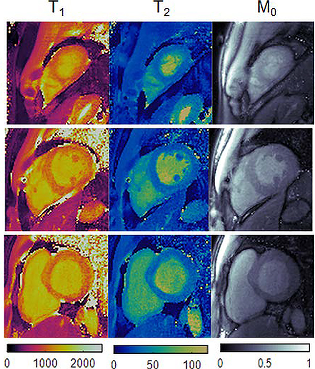
Cardiac Magnetic Resonance Fingerprinting was modified for simultaneous multislice acquisitions. The sequence employs multiband RF pulses with a different RF phase schedule applied to each slice. When combined with a low rank reconstruction, simultaneous T₁, T₂, and M₀ maps from three slices can be acquired in vivo during one breathhold.

Introduction

Mapping of relaxation times offers valuable information in cardiac imaging. Measurements of T₁ and T₂ provide insight into many pathologies, including myocardial scarring,^1,2 inflammation,³ early transplant rejection,⁴ amyloidosis,⁵ fibrosis,⁶ infarct,⁷ and edema.^8,9 Quantitative data may enable clinicians to make objective decisions regarding diagnosis and monitoring of disease. Conventional methods for measuring T₁ in the heart are based on inversion and saturation recovery experiments, including the family of methods derived from MOLLI^10,11 and SASHA.¹² Myocardial T₂ is typically measured using fast spin echo^13,14 or gradient echo sequences with multiple T₂ preparation times.^8,15

One disadvantage of the abovementioned sequences is that mapping each tissue property usually requires a separate breathheld scan. Several methods have recently been proposed that map T₁ and T₂ simultaneously, including CABIRIA,¹⁶ QALAS,^17,18 joint T₁-T₂ mapping,¹⁹ and Magnetic Resonance Fingerprinting (MRF).^20,21 MRF diverges from the traditional paradigm of collecting recovery or decay curves and fitting single pixel signals to an exponential model to extract T₁ and T₂ values. Instead, MRF employs a pulse sequence with variable parameters to encode different tissues, which have different underlying T₁ and T₂ values, with distinct signal evolutions. A dictionary of simulated signals for thousands of combinations of T₁ and T₂ is created using the Bloch equations. Pattern matching is performed between the acquired signal at each pixel and the dictionary to find the best matching dictionary entry, which indicates the T₁ and T₂ measurement for that pixel.

MRF has several advantages over conventional mapping. First, pattern matching is robust to many sources of error, including aliasing artifacts caused by undersampling k-space. Thus, MRF scans can be highly accelerated, leading to short scan times. One undersampled MRF image is acquired every TR (approximately 5ms). Signal dynamics can thus be sampled at a high temporal resolution, which may help to accurately measure T₁ and T₂. Cardiac MRF (cMRF) has been shown to be insensitive to heart rate variability within the scan because the subject’s own electrocardiogram (ECG) is used when creating the dictionary.²¹

Although cMRF is efficient for jointly mapping myocardial T₁, T₂, and proton density (M₀), each slice must be acquired in a separate breathhold. Whole-heart coverage would require many repeated breathholds, which is not feasible in a time-constrained cardiac MR exam. However, whole-heart mapping is desirable since limited slice coverage risks missing focal pathology.

Previous studies have improved MRF slice coverage for neuroimaging by using simultaneous multislice (SMS) techniques. One study used a dualband acquisition with different RF phases and flip angles for each slice.²² SMS data were separated using pattern recognition by matching the slice-collapsed images to a different dictionary simulated for each slice. Other groups have achieved multiband (MB) factors of 2 using blipped-CAIPIRINHA²³ with slice SENSE²⁴, and MB=3 using blipped-CAIPIRINHA with through-time spiral GRAPPA to perform slice unaliasing.^25,26

In the original MRF work, quantitative maps were generated by computing the inner product between measured signal timecourses and the dictionary to find the best-matching timecourse, and thus T₁ and T₂ value, for each voxel. Recently, more advanced MRF reconstruction techniques have been introduced to improve accuracy and precision or reduce scan time. One class of techniques exploits low rank properties of the data. Such methods have previously been proposed for quantitative T₁ and T₂ mapping.^27–29 In MRF, the signal timecourses in the dictionary are correlated and therefore can be compressed along time. In this work, the reconstruction exploits a subspace calculated from the singular value decomposition (SVD) of the cMRF dictionary.³⁰ Images in this compressed space, which are called “coefficient images”,³¹ are calculated iteratively using nonlinear conjugate descent. Each iteration consists of (1) projection of undersampled k-space data from the time domain to the SVD subspace, (2) gridding and coil combination to yield the coefficient images, (3) wavelet denoising, (4) inverse gridding from the image domain to spiral k-space, and (5) projection of k-space data from the SVD subspace to the time domain. Pattern matching is performed only once after all iterations have completed. The method proposed by Assländer, et al, formulates the reconstruction problem in the same way.³² However, it is solved using a different algorithm (ADMM), and pattern matching between the coefficient images and compressed dictionary is performed every iteration. The method proposed by Zhao, et al. also exploits a subspace derived from the dictionary.³³ However, this reconstruction additionally takes advantages of spatiotemporal correlations between the multiple contrast-weighted MRF images, which is not done in this study. Finally, the technique introduced by Doneva, et al, calculates a subspace using a fully-sampled calibration region in k-space.³⁴ All computations are done in k-space, which is computationally efficient, but image-based sparsity constraints cannot be applied as done here.

This study aims to improve the efficiency and slice coverage of cMRF by combining it with SMS techniques to map myocardial T₁, T₂, and M₀ over three slices during one 16-heartbeat breathhold. Each slice is encoded with a unique signal evolution using multiband excitation and RF phase cycling, as in POMP³⁵ or CAIPIRINHA.³⁶ A low rank reconstruction is applied to the slice-collapsed and undersampled images to reduce aliasing artifacts before pattern matching. The proposed SMS cMRF reconstruction is explored in numerical simulations and is validated using the ISMRM/NIST system phantom. In vivo cardiac scans were collected in ten volunteers at 3T to assess the agreement between SMS cMRF with a multiband factor of 3, single-slice cMRF, and conventional cardiac mapping sequences.

Experimental

Pulse Sequence and Data Sampling

A detailed description of the cMRF pulse sequence used in this study has been published previously.^21,37 Briefly, the sequence is ECG-triggered with data collection in diastole to reduce cardiac motion artifacts. Every heartbeat contains a trigger delay that is adjusted based on the subject’s heart rate. During some heartbeats, a non-selective magnetization preparation pulse is applied after the trigger delay—either an inversion or T₂ preparation pulse with variable TIs (21–400ms) or TEs (40–80ms), respectively. Inversions are implemented using an adiabatic hyperbolic secant pulse (11ms duration). The T₂ preparation module consists of a 90°_x tip-down excitation (rectangular pulse, 0.5ms duration), four MLEV-weighted refocusing pulses (each is a composite 90°_x 180°_y 90°_x), and a 90°_−x tip-up excitation (composite 270°_x[−360°_x], 3.5ms duration). The time between the tip-down and tip-up excitations is given by the T₂ preparation time (TE). This type of T₂ preparation has been shown to be robust to B₀ and B₁⁺ inhomogeneities.^38–40 After the preparation pulse, data are collected during a fixed-duration scan window using a FISP-based readout.⁴¹ There is an unbalanced gradient moment along the slice-select axis after each TR, which produces dephasing across the voxel but does not eliminate the transverse magnetization. FISP-MRF is suitable for cardiac mapping at 3T because it is insensitive to off-resonance frequencies; thus, this property does not need to be modeled in the dictionary. Variable flip angles between 4–15° with a constant TR of 5.3ms are applied during the scan window. Forty-eight TRs are acquired every heartbeat, which results in a scan window of 5.3×48=255ms. The total scan duration is 16 heartbeats, and all data are collected during a breathhold.

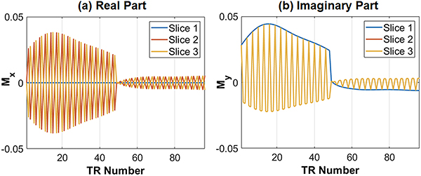
SMS excitation is achieved using a multiband sinc RF pulse with time bandwidth product 2 and a duration of 0.8ms. The same flip angle series is applied to all slices. In order to separate signals that originate from different slices, the RF phase is cycled as in POMP³⁵ or CAIPIRINHA.^36,42 For example, the RF phase for MB=3 at each TR is (0°,0°,0°,…) for slice 1; (0°,120°,240°,…) for slice 2; and (0°,240°,120°,…) for slice 3. Figure 1 illustrates simulated signal timecourses from three simultaneously excited slices with relaxation times of T₁=1400ms and T₂=50ms, which is representative of myocardium at 3T. The complex-valued signals from each slice are distinguishable because of the RF phase cycling and can potentially be separated by pattern recognition alone, as demonstrated previously.²²

Figure 1.

Examples of SMS cMRF signal evolutions with MB=3 for a fixed T₁=1400ms and T₂=50ms, which is similar to the relaxation times in myocardial tissue at 3T. (a) The signal timecourse for each slice has different real parts, and (b) the imaginary part for slice 1 is different from that for slices 2 and 3 (which overlap). For clarity, only the first two heartbeats (96 TRs) of the cMRF sequence are shown.

The k-space data are acquired using a variable density spiral trajectory with 0^th moment compensation, maximum slew rate 170 T/m/s, maximum gradient amplitude 23.4 mT/m, 300mm² FoV, 192×192 matrix, and 1.6mm² in-plane resolution.⁴³ The spiral has 48 interleaves with only 24 interleaves needed to fully sample the central 25% area of k-space. Undersampled images are gridded every TR using the NUFFT.⁴⁴ The trajectory rotates by approximately the golden angle every TR, which distributes aliasing artifacts incoherently through time.⁴⁵ The spiral gradient waveforms are provided in the Supplementary Material (SpiralGradient_300FoV_192Matrix_24inner_48outer.mat).

Dictionary Generation

A dictionary for each slice is generated using a Bloch equation simulation with input ranges for T₁ of [10:10:2000 2020:20:3000 3100:100:4000]ms and T₂ [2:2:100 105:5:250 260:10:500 520:20:600]ms. Non-physical combinations with T₂ < T₁ were excluded. As described above, each slice is excited with a unique sequence of RF phases. RF phase cycling causes the cMRF signal timecourses from different slices to appear distinct even if the underlying T₁ and T₂ values are the same. A separate dictionary is simulated for each slice which takes the RF phase into account. As will be described later, pattern matching is performed between the slice-collapsed data and each of the slice-specific dictionaries to generate maps for each slice.

Each dictionary has 26,665 entries and occupies 142MB in memory. To account for unavoidable physiological changes in heart rate during each scan, which will alter the relaxation between imaging periods and thus the shape of the cMRF timecourses, new dictionaries are generated after every scan using the exact sequence timing based on the subject’s heartrate.²¹ Two additional corrections are included in the dictionary, as recommended in prior work.³⁷ First, the non-rectangular slice profile is incorporated in the Bloch simulation.^46–48 To this end, the RF and gradient waveforms are simulated in the sequence programming environment. Next, a Bloch simulation is performed using these RF and gradient waveforms with 500 spins distributed across the slice direction. Signal timecourses are simulated independently for each spin, and the corrected dictionary is obtained by performing a complex sum over all spins. The second correction models the effects of relaxation during the inversion and T₂ preparation pulses, which can cause slight errors in the quantitative maps if not considered. This correction is performed in a similar fashion as the slice profile correction, using RF and gradient waveforms for the preparation pulses simulated within the sequence programming environment. The dictionary generation code was distributed to 8 nodes on a high-performance cluster with 12 CPU cores per node running MATLAB Mex code. The dictionary generation time was approximately 10 minutes per slice.

Low Rank Reconstruction

In this study, data are acquired using a high net acceleration factor (R=48 in-plane and up to MB=6). A low rank reconstruction is performed before pattern matching to reduce aliasing artifacts that could otherwise propagate through to the tissue property maps. The reconstruction is similar to existing low rank reconstructions for MRF.^32,33 The reconstruction is written as a constrained minimization problem

$$\underset{\tilde{x}}{\mathit{min}}{‖y-\sum _{i=1}^{NS}PFS{U}_{i,K}^H{\tilde{x}}_i‖}_2^2+\lambda \sum _{i=1}^{NS}R\left({\tilde{x}}_i\right)$$ (1)

In Eq. (1), y is the acquired slice-collapsed k-space data, P is a mask that samples the appropriate spiral interleaf every TR, F is the NUFFT operator, S is the coil sensitivity maps, and NS is the number of simultaneously excited slices. The matrix U_i is the left singular matrix obtained after performing the SVD along time of the dictionary for slice i, which is denoted D_i. Previously, SVD compression has been used to reduce the computation time needed for pattern matching in MRF.³⁰ Here, the SVD is used in an iterative framework to enforce consistency between cMRF measurements and the dictionary. After computing the SVD, all but the first K columns of the left singular matrix U_i are retained to yield the projection matrix U_i,K. The dictionary for each slice can be compressed along time by multiplication with the projection matrix

$$D_{i,K}=U_{i,K}{D}_i$$ (2)

Likewise, the undersampled cMRF images for slice i, denoted by x_i, can be compressed along time to produce coefficient images

$${\tilde{x}}_i=U_K{x}_i$$ (3)

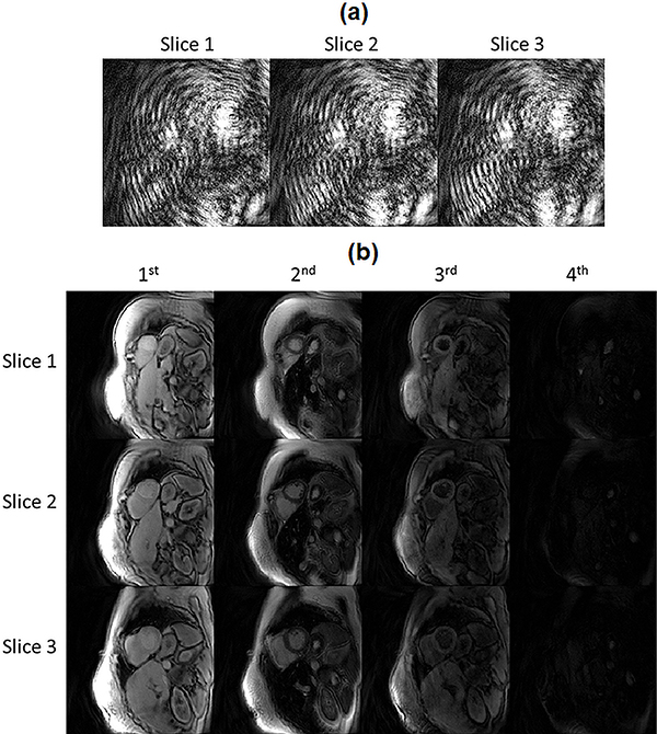
The dimensions of x_i are N_y × N_x × T and the dimensions of ${\tilde{x}}_i$ are N_y × N_x × K, where N_y and N_x are the number of pixels along the y and x dimensions, respectively, and T is the number of time points in the uncompressed dictionary. Figure 2 compares the undersampled images x_i, which are in the time domain, and the coefficient images ${\tilde{x}}_i$, which are in the dictionary-derived subspace.

Figure 2.

Comparison of undersampled images in the time domain and in the low-dimensional, dictionary-derived subspace from an SMS cMRF acquisition with MB=3. (a) An image frame corresponding to TR #20 after demodulating the undersampled SMS k-space by the RF phase (for each slice) and gridding. The images contain severe aliasing artifacts due to the 3-fold slice acceleration and 48-fold in-plane acceleration. (b) Examples of coefficient images derived by projecting the undersampled images onto the low-dimensional subspace calculated from each slice’s dictionary. The first four coefficient images are displayed for each slice, which correspond to the four largest singular values.

Wavelets are used as an l₁-sparsifying transform along the x- and y-spatial dimensions of the coefficient images, denoted by R in Eq. (1). Daubechies wavelets are used with four vanishing moments and six decomposition levels. Spatial regularization is not applied along the slice direction since there may be appreciable differences in image content between adjacent slices (i.e. due to a large slice gap). Using a smaller value for the coefficient λ in Eq. (1) gives more weight to the data consistency term and less weight to the sparsity term, and vice versa. The same value of λ was used for all reconstructions in this study, with λ = 0.002 times the maximum intensity in first coefficient image over all slices. This value was selected based on visual inspection after reconstructing a few in vivo datasets with different values of λ, using noise suppression and preservation of fine anatomical features as selection criteria. Supporting Figure 1 shows an example of maps reconstructed with different amounts of wavelet regularization.

Coil sensitivity maps are estimated using the demodulated SMS k-space data. For each TR, the SMS k-space is multiplied by the complex conjugate of the RF phase; this step is repeated for every individual slice. Next, the data are summed over time and gridded to yield a composite image for each slice that is largely free from aliasing artifacts. Finally, coil sensitivity maps for each slice are estimated using ESPIRiT (calibration region 30×30, kernel size 6×6).⁴⁹

The reconstruction is implemented in MATLAB (MathWorks, Natick, MA) using nonlinear conjugate gradient descent with backtracking line search, based off open-source code.^50,51 The number of iterations was fixed at 50 based on empirical convergence.

Pattern Matching

After applying the low rank reconstruction, tissue property maps are computed using inner product matching.^20,30 At each pixel location, the inner product is computed between the reconstructed coefficient images ${\tilde{x}}_i$ for a given slice i and the compressed dictionary for that slice, D_i,K. Maps are generated using the T₁ and T₂ values corresponding to the dictionary entry that maximizes the inner product. M₀ is calculated as the scaling factor between the measured data and the best-matching dictionary entry.

Numerical Simulations

Numerical phantom simulations were performed to evaluate the T₁ and T₂ quantification accuracy of the proposed SMS cMRF technique at different multiband factors from MB=1 (i.e. single-slice) up to MB=6. The aim of this experiment was to investigate the maximum MB factor that could potentially be achieved within a breathhold lasting 16 heartbeats, which is the scan time used in the original cMRF work. A numerical phantom with multiple slices and a range of T₁, T₂, and proton density values was desired. Because the scan is breathheld and ECG-triggered, the data should ideally contain no respiratory or cardiac motion, and the choice of phantom structure is immaterial. Because no cardiac phantom was readily available, an abdominal relaxation phantom was used instead.⁵² The phantom contains up to six slices through the abdomen, which are numbered consecutively so that slice 1 is used for MB=1, slices 1 and 2 for MB=2, and so on.

First, for each MB factor, a separate dictionary was simulated for each slice that differs only in the RF phase pattern. The pulse sequence was simulated with fixed timings corresponding to a steady 60bpm heart rate. Reference images were generated by inserting the appropriate timecourses from the dictionary at each pixel location. Next, the reference images were multiplied by coil sensitivity maps to generate multi-channel data. The sensitivity maps were simulated with 24 channels over 6 slices, with 3 rings of 8 circularly arranged coils. Then the multichannel images were resampled along the spiral trajectory, and the k-space data were summed over the slice direction to mimic an SMS acquisition.

Tissue property maps were reconstructed in two ways. In the first method, coefficient images generated from the low rank reconstruction were then matched to their slice-specific dictionaries after SVD compression using inner product matching. The rank K in Eq. (1–3) was selected automatically by finding all singular values that are greater than 2% of the first (maximum) singular value. For this pulse sequence, K=7 was used. In the second method, tissue property maps were computed using “direct matching”. This technique is equivalent to the first iteration of the low rank reconstruction. The SMS k-space data were demodulated by multiplication with the complex conjugate of the RF phase for each slice at every TR. Next the slice-separated k-space data were gridded to the image domain. After SVD compression, the coefficient images from each slice were matched to the slice-specific dictionaries using inner product matching.

To assess robustness to noise, the simulations were repeated after adding progressively larger amounts of complex Gaussian noise in k-space with standard deviation σ_N scaled by 0.0, 0.5, 1, and 2% of the maximum amplitude of the direct current (DC) signal in k-space over the entire acquisition. Errors were quantified by computing the normalized root mean square error (RMSE) in the T₁ and T₂ maps over all regions with non-zero spin density. RMSE values are reported after averaging over all the simultaneously acquired slices.

Phantom Validation

A validation experiment was performed by scanning the ISMRM/NIST MRI system phantom at 3T (Siemens MAGNETOM Skyra, Erlangen, Germany) using an 18-channel head coil array.⁵³ The T₂ array of the phantom was analyzed because it contains physiologically relevant ranges for both T₁ (91–2480ms) and T₂ (6–581ms). Data were acquired using single-slice cMRF (i.e. MB=1) and SMS cMRF from MB=2 to MB=6. The same scan parameters were used as in the simulation study. A steady 60bpm heart rate simulated at the scanner with a diastolic scan window of 255ms. The slice thickness was 8mm with the slice gap fixed at 24mm for all multiband factors. Other relevant scan parameters include: matrix size 192×192, FoV 300mm², in-plane resolution 1.6×1.6mm², variable flip angles 4–15° (sinc RF excitation pulses with time bandwidth product 2 and 0.8ms duration), and constant TR/TE=5.3/1.39ms. For the SMS acquisitions, the scan planes were oriented so that the T₂ array was imaged within the centermost slice in the slice group. T₁, T₂, and M₀ maps were reconstructed both after performing the low rank reconstruction and using direct matching.

The maps were analyzed by drawing 5×5 ROIs within each phantom sphere in the slice containing the T₂ array and computing the mean and standard deviation in T₁ and T₂. NMR T₁ and T₂ measurements provided by NIST were used as the gold standard values. For each MB factor, the concordance correlation coefficient (CCC) was computed⁵⁴ and a linear regression performed between the reference and cMRF measurements. For each MB factor, precision was assessed using the coefficient of variation (CoV), defined as the standard deviation in T₁ or T₂ in each ROI divided by the reference value.

Computation times for both reconstruction methods were also recorded each MB factor from 1 through 6. For direct matching, this includes the time for SVD compression of the undersampled data in k-space, gridding, and pattern matching. For the low rank reconstruction, this includes the time to iteratively solve Eq. (1) and then perform pattern matching.

In Vivo Cardiac Mapping

Ten healthy volunteers were enrolled in this IRB-approved, HIPAA-compliant study after obtaining written informed consent. Short-axis cardiac scans were performed at 3T using an 18-channel body coil array and 12 channels from the spine array. All cMRF scans were performed with the same parameters as the phantom experiments. The ECG trigger delay was adjusted for each subject’s heart rate to place the scan window in diastole. Cardiac shimming was performed using a shim volume centered tightly around the heart. Three slice positions were selected to cover apical, medial, and basal levels of the heart. A slice thickness of 8mm was used with 20–24mm slice gap, depending on the size of the heart. One SMS cMRF scan was acquired with MB=3 during a 16-heartbeat breathhold. For comparison, separate single-slice cMRF scans were performed at the same slice positions in three separate 16-heartbeat breathholds. Conventional T₁ and T₂ maps were also collected using the Siemens MyoMaps software package.⁵⁵ Apical, medial, and basal T₁ maps were acquired in separate MOLLI scans using the 5(3)3 version of the sequence.^10,56 Similarly, T₂ maps were acquired using T₂-prepared FLASH with a 1(3)1(3)1 acquisition pattern and three echo times of 0 (i.e. no T₂ preparation), 25, and 55ms. For both conventional mapping scans, a GRAPPA acceleration factor of R=2 was used (36 calibration lines) with 6/8 Partial Fourier, a scan window of 306ms, 192×192 matrix, and 300mm² FoV. The conventional maps were reconstructed using nonlinear parameter fitting.

ROIs were drawn separately on the T₁ and T₂ maps within AHA-defined myocardial segments numbered 1–16. To assess the agreement between conventional mapping, single-slice cMRF, and SMS cMRF, the T₁ and T₂ values within each segment were first averaged for each volunteer, and then the mean and standard deviation of T₁ and T₂ values among the volunteers were calculated. For each AHA segment, one-way ANOVA tests followed by Tukey’ honestly significant difference (HSD) post-hoc tests were performed at a p<0.05 significance level to assess if single-slice cMRF, SMS cMRF, and MOLLI (or T₂-prepared FLASH) yield the same mean T₁ (or T₂) values. A similar statistical analysis was performed using ROIs manually drawn over the entire slice at basal, medial, and apical slice positions. To assess the precision of each technique, the CoV in the T₁ and T₂ maps were computed over the entire slice for each volunteer. One-way ANOVA tests followed by Tukey’s HSD post-hoc tests were conducted to assess if there were significant (p<0.05) differences in CoV measurements between single-slice cMRF, SMS cMRF, and conventional techniques.

Results

Numerical Simulations

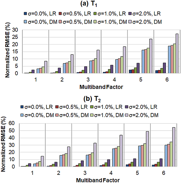
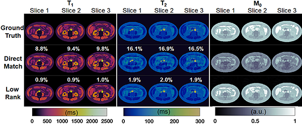
Results from the numerical simulations are shown in Figure 3. RMSE values in the T₁ and T₂ maps are plotted for different MB factors and for different amounts of added noise, and results are shown for both direct matching and the low rank reconstruction. First, the errors in T₁ and T₂ quantification progressively increase at higher MB factors, regardless of reconstruction method. Second, for a fixed MB factor, the T₁ and T₂ RMSE values monotonically increase as more noise is added to the raw data. Third, the low rank reconstruction consistently yields more accurate T₁ and T₂ estimations compared to direct matching at all MB factors (even for single-slice cMRF) and noise levels. For example, at MB=3 with noise level σ_N = 0.5% of the DC signal, the RMSE values for the low rank reconstruction (T₁ RMSE 0.9%, T₂ RMSE 2.0%) are much smaller than those for direct matching (T₁ RMSE 9.1%, 17.2%). This can be seen visually in Figure 4, which shows tissue property maps from three slices of the digital phantom simulated with an MB factor of 3. Visible aliasing artifacts and quantitative errors are seen in the T₁, T₂, and M₀ maps in the direct matching reconstruction; however, these artifacts are largely removed after the low rank reconstruction.

Figure 3.

RMSE values in the SMS cMRF maps from numerical simulations for (a) T₁ and (b) T₂. Results are presented for two direct matching (DM) and the low rank MRF reconstruction (LR). In addition, simulations were repeated after adding different amounts of noise in k-space. The value of σ denotes the standard deviation as a percentage of the maximum amplitude of the direct current (DC) signal in k-space over the entire acquisition.

Figure 4.

SMS cMRF maps from the numerical simulation with MB factor 3. T₁, T₂, and M₀ maps over three slices from the digital phantom are shown from the ground truth reference (top row), after direct matching (middle row), and after the low rank reconstruction (bottom row). The normalized RMSE in the T₁ and T₂ maps for each slice are also displayed.

Phantom Validation

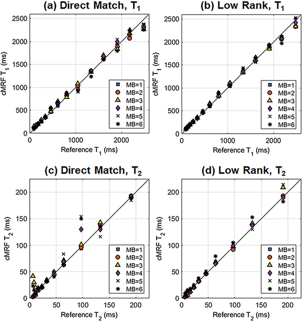
Figure 5 shows a scatterplot of the ISMRM/NIST phantom reference T₁ and T₂ values plotted against cMRF measurements at different MB factors. Table 1 presents the slope, y-intercept, and coefficient of determination (R²) for the best-fit line in each case. T₁ was quantified accurately even up to the highest MB factor acquired (MB=6). A strong linear agreement with reference T₁ values was obtained even with direct matching, where all R² values were above 0.99. The low rank reconstruction slightly improves the accuracy; for example, at MB=3, the low rank reconstruction yields a slightly higher R² than direct matching (0.998 vs 0.994). Overall, T₂ quantification was more challenging. Direct matching yielded an excellent linear correlation for MB=1 and MB=2 (R² above 0.999). However, it produced a weaker correlation at MB=3, with the best-fit line having R²=0.919, slope 1.37, and y-intercept 6.3ms. The low rank reconstruction yielded a more accurate T₂ quantification. At MB=3, the R² increased to 0.999, with the slope of the best-fit line closer to 1 (specifically 1.08) and the y-intercept closer to 0 (specifically 2.5ms). Table 2 shows CCC values between the reference and SMS cMRF measurements. The T₁ CCC values are above 0.99 for all MB factors and for both direct matching and low rank methods. The T₂ CCC values decrease when moving from MB=2 (CCC 0.999) to MB=3 (CCC 0.900) with direct matching. The low rank reconstruction results in correlations closer to 1; for instance, at MB=3, the CCC increases to 0.996.

Figure 5.

Scatterplot between reference and SMS cMRF T₁ and T₂ measurements in the T₂ array of the ISMRM/NIST system phantom at 3T. SMS cMRF data were acquired with MB factors from 1 (i.e. single-slice) to 6. Results are shown for (a) T₁ using direct matching, (b) T₁ after the low rank reconstruction, (c) T₂ using direct matching, and (d) T₂ after the low rank reconstruction.

Table 1.

Linear regression results from the NIST phantom experiment between reference and cardiac MRF T₁ and T₂ measurements. Scans were performed with multiband factors between 1 and 6, and maps were generated using either direct matching or a low rank MRF reconstruction. The table displays the slope, y-intercept, and R² values of the best-fit line between the reference and cMRF data.

			MB=1	MB=2	MB=3	MB=4	MB=5	MB=6
T1	Direct Match	Slope	0.97	0.95	0.94	0.97	0.98	0.93
		Intercept	28.4	45.6	63.3	48.1	30.2	56.7
		R2	0.998	0.998	0.994	0.992	0.993	0.991
	Low Rank	Slope	0.96	0.94	0.95	0.97	0.99	0.98
		Intercept	29.2	42.2	48.1	39.5	20.2	32.5
		R2	0.998	0.999	0.998	0.997	0.997	0.994
T2	Direct Match	Slope	1.01	1.00	1.37	0.91	0.87	0.85
		Intercept	−2.4	−1.6	−6.3	6.2	9.8	12.4
		R2	1.000	0.999	0.919	0.970	0.921	0.926
	Low Rank	Slope	0.96	1.01	1.08	0.96	1.03	1.02
		Intercept	0.1	−2.4	−2.5	1.8	0.9	4.4
		R2	0.996	0.999	0.999	0.997	0.994	0.993

Table 2.

Concordance correlation coefficients (CCC) from the ISMRM/NIST phantom experiment for T₁ and T₂ maps collected with SMS cardiac MRF. Data are shown for multiband factors up to MB=6. Maps were generated using both direct matching and the low rank MRF reconstruction.

		Multiband Factor
		1	2	3	4	5	6
T1	Direct Match	0.999	0.997	0.995	0.996	0.997	0.993
	Low Rank	0.998	0.998	0.998	0.998	0.998	0.997
T2	Direct Match	1.000	0.999	0.900	0.982	0.955	0.955
	Low Rank	0.998	0.999	0.996	0.998	0.996	0.996

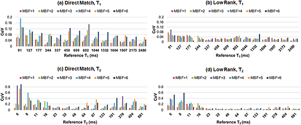
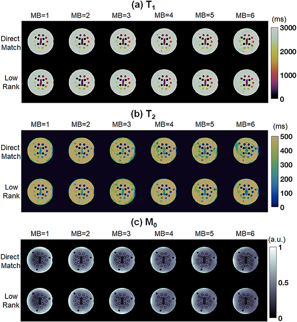
Results from the precision analysis are shown in Figure 6, which plots the CoV for various MB factors. With direct matching, the T₁ CoV generally increases at higher MB factors. With direct matching, the precision in T₂ is fairly stable up to MB=3 for intermediate T₂ values (e.g. 23–133m) but becomes worse at higher MB factors. Overall, the low rank reconstruction yields more precise T₁ and T₂ measurements than direct matching for both single-slice and SMS cMRF. The T₁ CoV is generally stable even up to MB=6, for T₂ the CoV values are fairly comparable up to MB=3. For a T₁ of 1332ms, which is close to the T₁ of myocardium, the CoV values for T₁ are 0.025 for direct matching MB=1, 0.020 for low rank MB=1, 0.033 for direct matching MB=3, and 0.027 for low rank MB=3. For a T₂ of 46ms, which is representative of myocardium, the CoV values for T₂ are 0.038 for direct matching MB=1, 0.038 for low rank MB=1, 0.039 for direct matching MB=3, and 0.22 for low rank MB=3. The CoV values for T₁ and T₂ are higher within ROIs having short T₂ of 16ms or less. Figure 7 shows maps from a slice through the T₂ array acquired with SMS cMRF using MB=1 through MB=6.

Figure 6.

Precision analysis from the NIST/ISMRM MRI system phantom experiment. SMS cMRF data were acquired with MB factors from 1 (i.e. single-slice) to 6. The coefficient of variation (CoV) was computed within fourteen ROIs in the T₂ array of the phantom. Results are shown for (a) T₁ using direct matching, (b) T₁ after the low rank reconstruction, (c) T₂ using direct matching, and (d) T₂ after the low rank reconstruction.

Figure 7.

Representative maps from the T₂ layer of NIST/ISMRM system phantom using SMS cMRF with MB factors from 1 to 6. Results are shown for (a) T₁, (b) T₂, and (c) M₀. For each tissue property, maps are displayed after direct matching (top row in each panel) and the low rank reconstruction (bottom row in each panel).

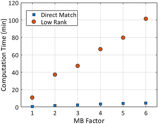
Computation times for direct matching and low rank reconstructions at different MB factors are presented in Figure 8. The reconstruction time for both methods increases linearly with MB factor. The low rank reconstruction took 15–20 times longer to complete than direct matching. Whereas direct matching took 0.7 minutes for MB=1 and 2.4 minutes for MB=3, the low rank reconstruction required 10.9 minutes for MB=1 and 47.3 minutes for MB=3. In addition, no restrictions due to SAR or RF amplifier limits occurred even at the maximum multiband factor tested (MB=6) due to the use of small flip angles.

Figure 8.

Computation times for SMS cMRF using direct matching and the low rank reconstruction. Times are reported for the phantom data, which had 768 time points and 18 channels. These times will depend on the cMRF sequence length and the number of channels.

In Vivo Cardiac Mapping

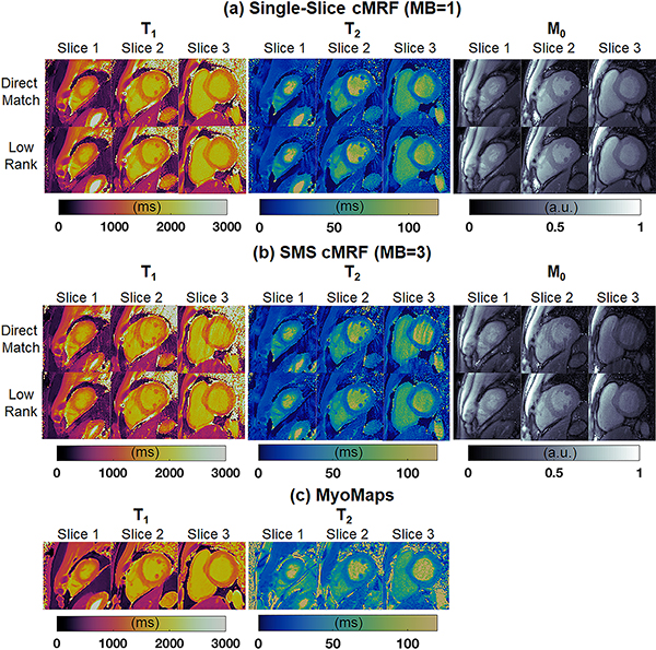
Quantitative scans were performed on ten healthy subjects at 3T. Representative maps from one volunteer are shown in Figure 9. Single-slice cMRF scans were repeated in three separate breathholds to cover apical, medial, and basal slices. High-quality maps were obtained with both direct matching and low rank reconstructions, with homogeneous myocardial wall measurements, well-defined papillary muscles, and few visible artifacts. SMS cMRF was also performed with MB=3 in one breathhold (i.e. 3-fold reduction in total scan time). Residual spiral aliasing artifacts are visible on the T₁, T₂, and M₀ maps using direct matching and are especially visible on the medial and basal slices. The low rank reconstruction reduces these artifacts and produces values that appear more homogeneous over the myocardial wall. From a visual inspection, the low rank MB=3 cMRF maps appear slightly noisier than the low rank MB=1 maps. Conventional single-slice T₁ maps acquired with MOLLI and T₂ maps acquired with T₂-prepared FLASH are also shown for comparison.

Figure 9.

Representative T₁, T₂, and M₀ maps from apical, medial, and basal slices in one volunteer at 3T. (a) Maps from three slices were acquired simultaneously using SMS cMRF with MB=3 during one breathhold. (b) Maps from collected during three separate breathholds (one per slice) using single-slice cMRF. (c) Maps collected using conventional cardiac mapping sequences—MOLLI for T₁, and T₂-prepared FLASH for T₂. These scans required six separate breathholds (one per slice with T₁ and T₂ acquired separately).

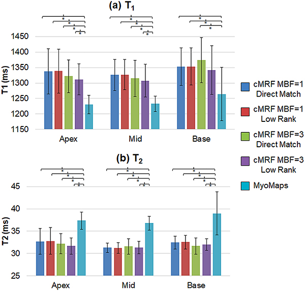
Figure 10 compares the slice-level T₁ and T₂ measurements acquired with cMRF (MB=1 and MB=3) and MyoMaps. The graphs show the mean relaxation times averaged over all volunteers, and the error bars indicate the standard deviation in mean T₁ or T₂ over all volunteers. No significant differences in mean T₁ or T₂ were observed between MB=1 and MB=3 cMRF at any slice position or between the direct matching and low rank reconstructions There was a significant difference (p<0.05) in T₁ measurements between MOLLI and cMRF (both MB=1 and MB=3) and between T₂-prepared FLASH and cMRF (both MB=1 and MB=3) at all slice positions. MOLLI T₁ values were lower than cMRF by roughly 100ms, and the conventionally acquired T₂ values were roughly 5ms higher than cMRF. With all cMRF scans, the T₂ measurements were consistent across all slice positions. cMRF T₁ measurements were slightly (20–50ms) higher in basal slices compared to medial and apical slices; similar trends in T₁ from basal to apical slices have been reported elsewhere.^57,58 A larger spread in T₁ and T₂ measurements was observed in basal slices for both cMRF (MB=1 and MB=3) and MyoMaps.

Figure 10.

Summary of slice-level myocardial relaxation times acquired with SMS cMRF (MB=3), single-slice cMRF, and conventional cardiac mapping sequences (MyoMaps). Results are shown for apical, medial, and basal slices and are presented for (a) T₁ and (b) T₂. The graph shows mean T₁ and T₂ values over all volunteers, and the error bars indicate standard deviations. A bracket with an asterisk (*) indicates a significant difference (p < 0.05) between groups from the one-way ANOVA with Tukey’s HSD post-hoc test.

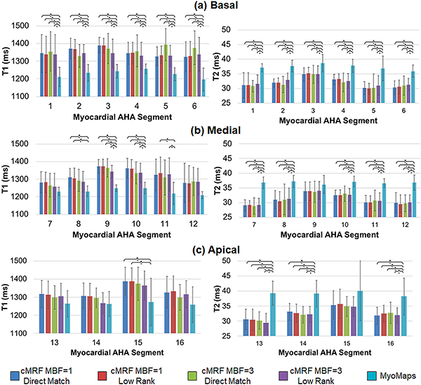
Figure 11 presents a similar analysis of the mean and standard deviation in T₁ and T₂ within the 16 AHA myocardial segments. There were no significant differences between MB=1 vs MB=3 cMRF, or between direct matching and low rank results. However, there were significant differences between MOLLI and cMRF (both MB=1 and MB=3) in basal segments 1–6, medial segments 8–11, and apical segment 15. There were also significant differences in T₂ between T₂-prepared FLASH and cMRF (both MB=1 and MB=3) in all segments except 9 and 15.

Figure 11.

Summary of relaxation times within each of the AHA-defined myocardial segments acquired with SMS cMRF (MB=3), single-slice cMRF, and conventional cardiac mapping sequences (MyoMaps). Maps were reconstructed using single-slice cMRF with direct matching (MBF=1, DM), single-slice cMRF with the low rank reconstruction (MBF=1, LR), SMS cMRF with MB=3 and direct matching (MBF=3, DM), SMS cMRF with MB=3 and the low rank reconstruction (MBF=3, LR), and conventional cardiac mapping sequences (MOLLI for T₁, and T₂-prepared FLASH for T₂). Results are shown for T₁ and T₂ in (a) basal, (b) medial, and (c) apical segments. The graph shows mean T₁ and T₂ values over all volunteers, and the error bars indicate standard deviations. A bracket with an asterisk (*) indicates a significant difference (p < 0.05) between groups from the one-way ANOVA with Tukey’s HSD post-hoc test.

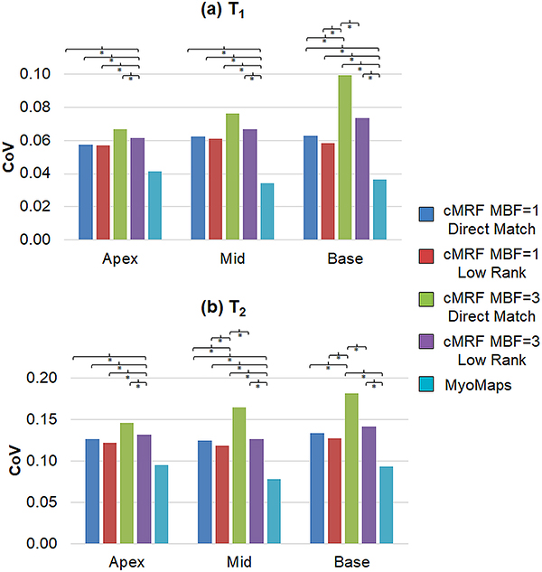
Measurement precision was assessed by comparing the CoV between different scans; a slice-wise summary is presented in Figure 12. For all slice positions, MOLLI CoV measurements were significantly smaller than cMRF regardless of MB factor or reconstruction method. At the basal slice, significantly higher T₁ CoV measurements were obtained using cMRF and direct matching at MB=3 vs MB=1. However, the low rank reconstruction with MB=3 yielded significantly smaller T₁ CoV values than direct matching with MB=3; and no significant differences were observed between low rank MB=3 and MB=1 (either direct matching or low rank). Similarly, for T₂, the conventional method yielded CoV values that were significantly smaller than cMRF at apical and medial slices regardless of MB factor or reconstruction method. They were also significantly smaller than cMRF with MB=3 but not MB=1 at the basal slice. At the medial and basal slices, CoV measurements with cMRF and direct matching were significantly higher at MB=3 versus MB=1. However, the low rank reconstruction with MB=3 yielded significantly smaller T₂ CoV values than direct matching with MB=3; and no significant differences were observed between low rank MB=3 and MB=1 (either direct matching or low rank).

Figure 12.

Precision as measured by the coefficient of variation (CoV) within basal, medial, and apical slices. Maps were reconstructed using single-slice cMRF with direct matching (MBF=1, DM), single-slice cMRF with the low rank reconstruction (MBF=1, LR), SMS cMRF with MB=3 and direct matching (MBF=3, DM), SMS cMRF with MB=3 and the low rank reconstruction (MBF=3, LR), and conventional cardiac mapping sequences (MOLLI for T₁, and T₂-prepared FLASH for T₂). Results are shown for (a) T₁ and (b) T_2. A bracket with an asterisk (*) indicates a significant difference (p < 0.05) between groups from the one-way ANOVA with Tukey’s HSD post-hoc test.

Discussion

In this study, the efficiency of cMRF was improved by combining cMRF with SMS techniques to achieve better slice coverage within the same scan time. Additionally, a low rank reconstruction was applied to improve the precision of cMRF as well as enable SMS acquisitions up to MB=3 in vivo. The first part of this study explored the maximum MB factor that could be achieved within one breathhold using numerical simulations. Next, the proposed technique was validated by scanning the ISMRM/NIST system phantom with different MB factors. Finally, in vivo cardiac scans were performed to demonstrate that T₁, T₂, and M₀ maps from three slices could be acquired simultaneously in one breathhold. The proposed method offers a three-fold reduction in scan time compared to single-slice cMRF. It is even more scan efficient compared to conventional cardiac mapping techniques, which typically measure T₁ or T₂ in separate breathholds. Finally, the T₁ and T₂ maps from SMS cMRF are co-registered at the same breathhold position across different slices because they are derived from the same dataset.

Two types of cMRF reconstructions were explored in this study. With direct matching, SMS k-space data are demodulated by the slice-specific RF phase, gridded, and matched to a slice-specific dictionary. This method is used for single-slice mapping in the original MRF work and is not iterative. The low rank technique iteratively reconstructs images using a subspace calculated from the temporal SVD of the dictionary. First, it was found that the low rank reconstruction yields better precision in the T₁ and T₂ maps than direct matching for both single-slice and SMS cMRF. Second, with single-slice data, the low rank reconstruction produces mean relaxation times that agree with direct matching results. Third, the low rank reconstruction improves the accuracy of SMS cMRF. Maps reconstructed with direct matching have artifacts at high MB factors (usually MB=3 and above), especially in the T₂ maps, due to the limited number of time frames acquired within the breathhold. The low rank reconstruction enables SMS acquisitions at these higher MB with reduced artifacts. This was observed in the phantom experiments where, for example, direct matching yielded a correlation of R²=0.919 between cMRF and reference T₂ values at MB=3, but the low rank reconstruction produced a higher correlation of R²=0.998. In the in vivo example in Figure 9, artifacts are less visible in the MB=3 low rank maps compared to direct matching.

This study also investigated the precision of SMS cMRF compared to single-slice cMRF and conventional cardiac mapping sequences. Overall, the conventional sequences outperformed cMRF in terms of precision regardless of MB factor or reconstruction technique. The comparatively high precision of the conventional methods may be due to smoothing filters applied to the tissue property maps, which could not be altered as they were generated using vendor-supplied software. With direct matching, SMS cMRF measurements had greater variability than single-slice cMRF measurements. However, the precision improved when using the low rank reconstruction. As seen in Figure 12, low rank SMS cMRF at MB=3 produced significantly smaller T₁ and T₂ CoV measurements compared to direct matching at MB=3. And whereas the CoV values for cMRF MB=3 with direct matching were significantly higher than MB=1 for basal and medial slices, the differences between cMRF with the low rank reconstruction at MB=3 versus MB=1 were not significant.

This loss in precision is a tradeoff for reducing the total acquisition time and is related to SNR and artifact level. With SMS imaging, the SNR is proportional to the square root of the number of simultaneously excited slices.⁵⁹ At first glance, this may suggest that SMS cMRF should have better precision than its single-slice counterpart. However, the higher net acceleration factor (due to the combination of in-plane and slice acceleration) may result in greater aliasing energy, which interferes with the pattern matching in cMRF and balances the SNR gain from SMS excitation.

Slice cross-talk could potentially introduce quantitative errors if the gap between adjacent simultaneously excited slices is small, and slice profile imperfections lead to mixed excitation of the multiple slices. In this study, the slice gap was intentionally set to be larger than 2.5 times the slice thickness. This value was chosen after simulating the slice profile of the multiband RF pulse and examining the minimum slice gap needed to avoid overlapping excitation. The slice gap could potentially be decreased in a few ways. First, a longer or more optimized RF pulse could be used to produce an excitation profile with a flatter top, sharper rolloff, and minimal sidelobes. Alternatively, the effects of slice cross-talk could be modeled in the dictionary simulation.

Conventional cardiac T₁ and T₂ mapping sequences were acquired in all volunteers for comparison with cMRF. Previous studies with MOLLI have reported myocardial T₁ values of 1050–1150ms at 3T.^11,60 It has been reported that MOLLI underestimates T₁ due to a variety of factors, including magnetization transfer, imperfect inversion efficiency, and sensitivity to off-resonance.^61–63 Saturation recovery mapping sequences, such as SASHA¹², are believed to be more accurate than inversion recovery techniques like MOLLI. At 3T, myocardial T₁ values with SASHA have been reported between 1477–1569ms.⁶⁴ In this study, the cMRF dictionary included corrections for some confounding factors that could introduce quantitative errors if not taken into account.³⁷ Specifically, the dictionary simulation modeled both the non-ideal slice profile, and T₁ and T₂ relaxation during the inversion and T₂ preparation pulses. With these corrections, both single-slice and SMS cMRF T₁ measurements were roughly 80–100ms higher than MOLLI (1320±52ms SMS cMRF with MB=3, 1340±46ms single-slice cMRF, and 1242±33ms MOLLI), although lower than literature ranges for SASHA. The remaining discrepancy between SASHA T₁ values may be explained by other confounding factors that are not yet modeled in the dictionary. The cMRF sequence used here relies heavily on inversion pulses for T₁ sensitivity, so magnetization transfer may result in shortened apparent myocardial T₁ values. T₂ measurements were consistent between single-slice and SMS cMRF. However, cMRF T₂ values in the heart were 5–6ms lower compared to the conventional T₂-prepared FLASH sequence (31.7±1.4ms SMS cMRF with MB=3, 32.2±1.5ms single-slice cMRF, and 37.7±2.3ms T₂-prepared FLASH). Similar discrepancies have been reported previously with FISP-based MRF in the brain.^65,66 The lower T₂ values may be due to a combination of magnetization transfer effects⁶⁷, motion sensitivity along the direction of the unbalanced gradient moment (i.e. slice direction), diffusion weighting from the spoiler gradient ⁶⁸, or intravoxel dephasing.⁶⁹

Cardiac MRF is one of several techniques proposed for joint myocardial T₁ and T₂ mapping.^16,17,19 Recently, CMR Multitasking has been reported for generating motion-resolved T₁ and T₂ maps with a scan time of 88s per slice.⁷⁰ In this novel method, data are acquired using a FLASH readout periodically interrupted by a combined inversion/T₂ prep pulse. Data are assigned to different respiratory and cardiac motion states using training data that are acquired every other TR. Maps are reconstructed using a low rank tensor model where the motion states and relaxation processes are treated as separate tensor dimensions. SMS cMRF differs from multi-tasking in several important regards. First, SMS cMRF generates maps from several slices simultaneously but only during a single cardiac and respiratory phase using ECG triggering and breathholding. Second, SMS cMRF uses a pulse sequence with a time-varying schedule of excitation flip angles, inversion pulses, and T₂ preparation pulses. Therefore, the signal evolutions need not conform to an exponential model, which could improve quantification of T₁ and T₂. Third, SMS cMRF explicitly performs pattern matching to a dictionary of simulated signal evolutions rather than fitting data to a nonlinear (exponential) model. Fourth, whereas multitasking uses a low rank tensor model, the reconstruction proposed in this study considers the dictionary as a matrix with low rank.

There are a few limitations to the current study. First, there are several physical effects that are not modeled when generating the cMRF dictionary which could introduce quantitative errors. As previously mentioned, magnetization transfer effects are not taken into account. No B₁⁺ corrections were performed, although previous work has shown that this particular cMRF sequence is relatively robust to B₁⁺ variations.³⁷ The slice profile correction that was included in the dictionary assumes there is only one tissue type across the slice direction of each voxel, and it does not consider partial volume or multi-compartment effects. The M₀ maps are currently weighted by the coil sensitivity profiles, as evidenced by the higher M₀ values obtained closer to the coil array near the chest wall (Figure 9). Finally, SMS cMRF required a relatively long breathhold of 16 heartbeats that may not be feasible for some patients. Failed breathholds can lead to artifacts in the parameter maps if the measured signals match to incorrect dictionary entries. In addition, through-plane respiratory motion will cause different tissues to move into the imaging planes, making it difficult to model the spin history in the dictionary.

Currently, the long computation times required for SMS cMRF are clinically prohibitive. A separate dictionary is simulated for every slice and also after every scan to accurately model the subject’s heart rate. Generating the dictionary currently takes 10 minutes per slice using a high-performance computing cluster, and the low rank reconstruction requires an additional 47 minutes to yield parameter maps for three slices. The computation time could potentially be shortened using optimized code and GPU or parallel programming. Recently, cardiac MRF has been presented using the open-source Gadgetron platform for online Bloch simulations and pattern matching.^71,72 This implementation takes less than two minutes to generate parameter maps at the scanner, and it could feasibly be extended to SMS.

One long-term goal of this work is to achieve whole-heart coverage during a single breathhold. Currently, the slice separation relies solely on RF phase cycling. It may be possible to achieve better slice separation at higher MB factors by applying different flip angle schedules to each slice, which has been demonstrated before.²² Additional encoding power could be obtained by also switching from non-selective to slice-selective preparation pulses. Each slice could then be excited with a unique schedule of inversion and T₂ preparation pulses to achieve more unique signal timecourses. Besides permitting higher MB factors, these strategies could potentially reduce the breathhold duration. Although this study demonstrates the technical feasibility of SMS cMRF in the heart, additional in vivo validation using a larger sample size across different sites should be performed, with comparisons to clinically established mapping sequences.

Conclusions

A method for simultaneous multislice excitation in cardiac MRF is presented in order to improve the slice coverage for simultaneous T₁, T₂, and M₀ quantification in the heart. The cMRF pulse sequence was modified to use multiband RF excitations. cMRF signal evolutions from different slices are separated by exciting each slice with a unique RF phase schedule, similar to POMP and CAIPIRINHA. A low rank MRF reconstruction is used to reduce the appearance of aliasing artifacts at these high net acceleration factors (due to the 48-fold in-plane acceleration combined with the slice acceleration). The feasibility of the proposed method is demonstrated in numerical simulations as well as phantom and in vivo cardiac scans of ten healthy volunteers at 3T. For single-slice acquisitions, the low rank reconstruction yields mean relaxation times that agree with direct matching results. Additionally, the low rank method improves the precision in T₁ and T₂ for both single-slice and SMS cMRF, and it enables the acquisition of maps with reduced artifacts at higher MB factors, up to MB=3 in vivo during a single breathhold. This represents a three-fold reduction in scan time compared to the original implementation of cMRF, which is designed to generate maps from just one slice during the same scan time. Compared to conventional cardiac mapping sequences, which generate single-slice maps of either T₁ or T₂ in separate acquisitions, SMS cMRF has the advantage of generating co-registered T1 and T₂ maps across several slices simultaneously.

Abbreviations

CAIPIRINHA

Controlled aliasing in parallel imaging results in higher acceleration

cMRF

Cardiac Magnetic Resonance Fingerprinting\

ECG

electrocardiogram

FLASH

Fast low angle shot

FoV

field of view

MB

multiband

MOLLI

Modified Look-Locker inversion recovery

MRF

Magnetic Resonance Fingerprinting

NUFFT

non-uniform fast Fourier transform

POMP

Phase-offset multiplanar

RF

radiofrequency

ROI

region of interest

SASHA

Saturation recovery single-shot acquisition

SMS

simultaneous multislice

SVD

singular value decomposition

TE

T₂ preparation time

TI

inversion time

TR

repetition time

References

- 1.Goldfarb JW, Arnold S, Han J. Recent myocardial infarction: assessment with unenhanced T1-weighted MR imaging. Radiology. 2007;245(1):245–250. [DOI] [PubMed] [Google Scholar]
- 2.Okur A, Kantarci M, Kizrak Y, et al. Quantitative evaluation of ischemic myocardial scar tissue by unenhanced T1 mapping using 3.0 Tesla MR scanner. Diagn Interv Radiol. 20(5):407–413. [DOI] [PMC free article] [PubMed] [Google Scholar]
- 3.Hinojar R, Nagel E, Puntmann VO. T1 mapping in myocarditis - headway to a new era for cardiovascular magnetic resonance. Expert Rev Cardiovasc Ther. 2015;13(8):871–874. [DOI] [PubMed] [Google Scholar]
- 4.Butler CR, Savu A, Bakal JA, et al. Correlation of cardiovascular magnetic resonance imaging findings and endomyocardial biopsy results in patients undergoing screening for heart transplant rejection. J Heart Lung Transplant. 2015;34(5):643–650. [DOI] [PubMed] [Google Scholar]
- 5.Karamitsos TD, Piechnik SK, Banypersad SM, et al. Noncontrast T1 mapping for the diagnosis of cardiac amyloidosis. JACC Cardiovasc Imaging. 2013;6(4):488–497. [DOI] [PubMed] [Google Scholar]
- 6.Bull S, White SK, Piechnik SK, et al. Human non-contrast T1 values and correlation with histology in diffuse fibrosis. Heart. 2013;99(13):932–937. [DOI] [PMC free article] [PubMed] [Google Scholar]
- 7.Dall’Armellina E, Piechnik SK, Ferreira VM, et al. Cardiovascular magnetic resonance by non contrast T1-mapping allows assessment of severity of injury in acute myocardial infarction. J Cardiovasc Magn Reson. 2012;14(1):15. [DOI] [PMC free article] [PubMed] [Google Scholar]
- 8.Giri S, Chung Y-C, Merchant A, et al. T2 quantification for improved detection of myocardial edema. J Cardiovasc Magn Reson. 2009;11:56. [DOI] [PMC free article] [PubMed] [Google Scholar]
- 9.Park CH, Choi E-Y, Kwon HM, et al. Quantitative T2 mapping for detecting myocardial edema after reperfusion of myocardial infarction: validation and comparison with T2-weighted images. Int J Cardiovasc Imaging. 2013;29 Suppl 1:65–72. [DOI] [PubMed] [Google Scholar]
- 10.Messroghli DR, Radjenovic A, Kozerke S, Higgins DM, Sivananthan MU, Ridgway JP. Modified look-locker inversion recovery (MOLLI) for high-resolution T 1 mapping of the heart. Magn Reson Med. 2004;52(1):141–146. [DOI] [PubMed] [Google Scholar]
- 11.Piechnik SK, Ferreira VM, Dall’Armellina E, et al. Shortened Modified Look-Locker Inversion recovery (ShMOLLI) for clinical myocardial T1-mapping at 1.5 and 3 T within a 9 heartbeat breathhold. J Cardiovasc Magn Reson 2010;12(1):69. [DOI] [PMC free article] [PubMed] [Google Scholar]
- 12.Chow K, Flewitt JA, Green JD, Pagano JJ, Friedrich MG, Thompson RB. Saturation recovery single-shot acquisition (SASHA) for myocardial T 1 mapping. Magn Reson Med. 2014;71(6):2082–2095. [DOI] [PubMed] [Google Scholar]
- 13.Marie PY, Angioï M, Carteaux JP, et al. Detection and prediction of acute heart transplant rejection with the myocardial T2 determination provided by a black-blood magnetic resonance imaging sequence. J Am Coll Cardiol. 2001;37(3):825–831. [DOI] [PubMed] [Google Scholar]
- 14.de Roquefeuil M, Vuissoz P-A, Escanyé J-M, Felblinger J. Effect of physiological heart rate variability on quantitative T2 measurement with ECG-gated Fast Spin Echo (FSE) sequence and its retrospective correction. Magn Reson Imaging. 2013;31(9):1559–1566. [DOI] [PubMed] [Google Scholar]
- 15.Huang TY, Liu YJ, Stemmer A, Poncelet BP. T2 measurement of the human myocardium using a T 2-prepared transient-state trueFISP sequence. Magn Reson Med. 2007;57:960–966. [DOI] [PubMed] [Google Scholar]
- 16.Santini F, Kawel-Boehm N, Greiser A, Bremerich J, Bieri O. Simultaneous T1 and T2 quantification of the myocardium using cardiac balanced-SSFP inversion recovery with interleaved sampling acquisition (CABIRIA). Magn Reson Med. 2015;74(2):365–371. [DOI] [PubMed] [Google Scholar]
- 17.Kvernby S, Warntjes MJ, Haraldsson H, Carlhall CJ, Engvall J, Ebbers T. Simultaneous three-dimensional myocardial T1 and T2 mapping in one breath hold with 3D-QALAS. J Cardiovasc Magn Reson. 2014;16:102. [DOI] [PMC free article] [PubMed] [Google Scholar]
- 18.Kvernby S, Warntjes M, Carlhall CJ, Engvall JE, Ebbers T. Single breath-hold 3D mapping of T1 and T2 relaxation times with 3D-QALAS-feasibility in patients. J Cardiovasc Magn Reson. 2015;17.25885056 [Google Scholar]
- 19.Akçakaya M, Weingärtner S, Basha TA, Roujol S, Bellm S, Nezafat R. Joint myocardial T1 and T2 mapping using a combination of saturation recovery and T2-preparation. Magn Reson Med. 2016;76(3):888–896. [DOI] [PMC free article] [PubMed] [Google Scholar]
- 20.Ma D, Gulani V, Seiberlich N, et al. Magnetic resonance fingerprinting. Nature. 2013;495(7440):187–192. [DOI] [PMC free article] [PubMed] [Google Scholar]
- 21.Hamilton JI, Jiang Y, Chen Y, et al. MR fingerprinting for rapid quantification of myocardial T1, T2, and proton spin density. Magn Reson Med. 2017;77:1446–1458. [DOI] [PMC free article] [PubMed] [Google Scholar]
- 22.Jiang Y, Ma D, Bhat H, et al. Use of pattern recognition for unaliasing simultaneously acquired slices in simultaneous multislice MR fingerprinting. Magn Reson Med. 2017;78(5):1870–1876. [DOI] [PMC free article] [PubMed] [Google Scholar]
- 23.Setsompop K, Gagoski BA, Polimeni JR, Witzel T, Wedeen VJ, Wald LL. Blipped-controlled aliasing in parallel imaging for simultaneous multislice echo planar imaging with reduced g-factor penalty. Magn Reson Med. 2012;67(5):1210–1224. [DOI] [PMC free article] [PubMed] [Google Scholar]
- 24.Larkman DJ, Hajnal JV., Herlihy AH, Coutts GA, Young IR, Ehnholm G. Use of multicoil arrays for separation of signal from multiple slices simultaneously excited. J Magn Reson Imaging. 2001;13(2):313–317. [DOI] [PubMed] [Google Scholar]
- 25.Seiberlich N, Lee G, Ehses P, Duerk JL, Gilkeson R, Griswold M. Improved temporal resolution in cardiac imaging using through-time spiral GRAPPA. Magn Reson Med. 2011;66(6):1682–1688. [DOI] [PMC free article] [PubMed] [Google Scholar]
- 26.Ye H, Cauley SF, Gagoski B, et al. Simultaneous multislice magnetic resonance fingerprinting (SMS-MRF) with direct-spiral slice-GRAPPA (ds-SG) reconstruction. Magn Reson Med. 2017;77(5):1966–1974. [DOI] [PMC free article] [PubMed] [Google Scholar]
- 27.Huang C, Graff CG, Clarkson EW, Bilgin A, Altbach MI. T2 mapping from highly undersampled data by reconstruction of principal component coefficient maps using compressed sensing. Magn Reson Med. 2012;67(5):1355–1366. [DOI] [PMC free article] [PubMed] [Google Scholar]
- 28.Zhao B, Lu W, Hitchens TK, Lam F, Ho C, Liang ZP. Accelerated MR parameter mapping with low-rank and sparsity constraints. Magn Reson Med. 2015;74(2):489–498. [DOI] [PMC free article] [PubMed] [Google Scholar]
- 29.Zhang T, Pauly JM, Levesque IR. Accelerating parameter mapping with a locally low rank constraint. Magn Reson Med. 2015;73(2):655–661. [DOI] [PMC free article] [PubMed] [Google Scholar]
- 30.McGivney DF, Pierre E, Ma D, et al. SVD compression for magnetic resonance fingerprinting in the time domain. IEEE Trans Med Imaging. 2014;33(12):2311–2322. [DOI] [PMC free article] [PubMed] [Google Scholar]
- 31.Tamir JI, Uecker M, Chen W, et al. T2 shuffling: Sharp, multicontrast, volumetric fast spin-echo imaging. Magn Reson Med. 2017;77(1):180–195. [DOI] [PMC free article] [PubMed] [Google Scholar]
- 32.Assländer J, Cloos MA, Knoll F, Sodickson DK, Hennig J, Lattanzi R. Low rank alternating direction method of multipliers reconstruction for MR fingerprinting. Magn Reson Med. 2018;79(1):83–96. [DOI] [PMC free article] [PubMed] [Google Scholar]
- 33.Zhao B, Bilgic B, Adalsteinsson E, Griswold MA, Wald LL, Setsompop K. Simultaneous multislice magnetic resonance fingerprinting with low-rank and subspace modeling. In: 2017 39th Annual International Conference of the IEEE Engineering in Medicine and Biology Society (EMBC) Vol 2017 IEEE; 2017:3264–3268. [DOI] [PMC free article] [PubMed] [Google Scholar]
- 34.Doneva M, Amthor T, Koken P, Sommer K, Börnert P. Matrix completion-based reconstruction for undersampled magnetic resonance fingerprinting data. Magn Reson Imaging. 2017;41:41–52. [DOI] [PubMed] [Google Scholar]
- 35.Glover GH. Phase‐offset multiplanar (POMP) volume imaging: A new technique. J Magn Reson Imaging. 1991;1(4):457–461. [DOI] [PubMed] [Google Scholar]
- 36.Breuer FA, Blaimer M, Heidemann RM, Mueller MF, Griswold MA, Jakob PM. Controlled aliasing in parallel imaging results in higher acceleration (CAIPIRINHA) for multi-slice imaging. Magn Reson Med. 2005;53(3):684–691. [DOI] [PubMed] [Google Scholar]
- 37.Hamilton JI, Jiang Y, Ma D, et al. Investigating and Reducing the Effects of Confounding Factors for Robust T1 and T2 Mapping with Cardiac MR Fingerprinting. Magn Reson Imaging. 2018;Submitted. [DOI] [PMC free article] [PubMed] [Google Scholar]
- 38.Jacobs JWM, Van Os JWM, Veeman WS. Broadband heteronuclear decoupling. J Magn Reson. 1983;51(1):56–66. [Google Scholar]
- 39.Shaka AJ, Rucker SP, Pines A. Iterative carr-purcell trains. J Magn Reson. 1988;77(3):606–611. [Google Scholar]
- 40.Brittain JH, Hu BS, Wright GA, Meyer CH, Macovski A, Nishimura DG. Coronary angiography with magnetization-prepared T2 contrast. Magn Reson Med. 1995;33:689–696. [DOI] [PubMed] [Google Scholar]
- 41.Jiang Y, Ma D, Seiberlich N, Gulani V, Griswold MA. MR fingerprinting using fast imaging with steady state precession (FISP) with spiral readout. Magn Reson Med. 2015;74(6):1621–1631. [DOI] [PMC free article] [PubMed] [Google Scholar]
- 42.Yutzy SR, Seiberlich N, Duerk JL, Griswold MA. Improvements in multislice parallel imaging using radial CAIPIRINHA. Magn Reson Med. 2011;65(6):1630–1637. [DOI] [PMC free article] [PubMed] [Google Scholar]
- 43.Hargreaves B Variable-Density Spiral Design Functions. http://mrsrl.stanford.edu/~brian/vdspiral/. Published 2005. Accessed June 1, 2017.
- 44.Fessler J, Sutton B. Nonuniform fast Fourier transforms using min-max interpolation. IEEE Trans Signal Process. 2003;51(2):560–574. [Google Scholar]
- 45.Winkelmann S, Schaeffter T, Koehler T, Eggers H, Doessel O. An optimal radial profile order based on the Golden Ratio for time-resolved MRI. IEEE Trans Med Imaging. 2007;26(1):68–76. [DOI] [PubMed] [Google Scholar]
- 46.Ma D, Coppo S, Chen Y, et al. Slice profile and B 1 corrections in 2D magnetic resonance fingerprinting. Magn Reson Med. 2017;78(5):1781–1789. [DOI] [PMC free article] [PubMed] [Google Scholar]
- 47.Hong T, Han D, Kim MO, Kim DH. RF slice profile effects in magnetic resonance fingerprinting. Magn Reson Imaging. 2017;41:73–79. [DOI] [PubMed] [Google Scholar]
- 48.Chiu S-C, Lin T-M, Lin J-M, et al. Effects of RF pulse profile and intra-voxel phase dispersion on MR fingerprinting with balanced SSFP readout. Magn Reson Imaging. 2017;41:80–86. [DOI] [PubMed] [Google Scholar]
- 49.Uecker M, Lai P, Murphy MJ, et al. ESPIRiT - An eigenvalue approach to autocalibrating parallel MRI: Where SENSE meets GRAPPA. Magn Reson Med. 2014;71(3):990–1001. [DOI] [PMC free article] [PubMed] [Google Scholar]
- 50.Lustig M, Donoho D, Pauly JM. Sparse MRI: The application of compressed sensing for rapid MR imaging. Magn Reson Med. 2007;58(6):1182–1195. [DOI] [PubMed] [Google Scholar]
- 51.Feng L, Axel L, Chandarana H, Block KT, Sodickson DK, Otazo R. XD-GRASP: Golden-angle radial MRI with reconstruction of extra motion-state dimensions using compressed sensing. Magn Reson Med. 2016;75(2):775–788. [DOI] [PMC free article] [PubMed] [Google Scholar]
- 52.Lo W-C, Chen Y, Jiang Y, Gulani V, Seiberlich N. Realistic 4D abdominal phantom for magnetic resonance imaging. In: Proceedings of the 25th Annual Meeting of ISMRM, Honolulu, HI, USA ; 2017:1231. [Google Scholar]
- 53.Russek SE, Boss M, Jackson EF, et al. Characterization of NIST/ISMRM MRI System Phantom. In: Proceedings of the 20th Annual Meeting of ISMRM ; 2012:2456. [Google Scholar]
- 54.Lin LI-K. A Concordance Correlation Coefficient to Evaluate Reproducibility. Biometrics. 1989;45(1):255. [PubMed] [Google Scholar]
- 55.Siemens Medical Solutions USA. MyoMaps. https://usa.healthcare.siemens.com/magnetic-resonance-imaging/options-and-upgrades/clinical-applications/myomaps. Published 2018. Accessed February 27, 2018. [Google Scholar]
- 56.Kellman P, Wilson JR, Xue H, Ugander M, Arai AE. Extracellular volume fraction mapping in the myocardium, part 1: evaluation of an automated method. J Cardiovasc Magn Reson. 2012;14(1):63. [DOI] [PMC free article] [PubMed] [Google Scholar]
- 57.Mygind ND, Michelsen MM, Pena A, et al. Coronary microvascular function and myocardial fibrosis in women with angina pectoris and no obstructive coronary artery disease: the iPOWER study. J Cardiovasc Magn Reson. 2016;18(1). [DOI] [PMC free article] [PubMed] [Google Scholar]
- 58.Choi EY, Hwang SH, Yoon YW, et al. Correction with blood T1 is essential when measuring post-contrast myocardial T1 value in patients with acute myocardial infarction. J Cardiovasc Magn Reson 2013;15(1). [DOI] [PMC free article] [PubMed] [Google Scholar]
- 59.Barth M, Breuer F, Koopmans PJ, Norris DG, Poser BA. Simultaneous multislice (SMS) imaging techniques. Magn Reson Med. 2016;75(1):63–81. [DOI] [PMC free article] [PubMed] [Google Scholar]
- 60.Dabir D, Child N, Kalra A, et al. Reference values for healthy human myocardium using a T1 mapping methodology: results from the International T1 Multicenter cardiovascular magnetic resonance study. J Cardiovasc Magn Reson. 2014;16(1):69. [DOI] [PMC free article] [PubMed] [Google Scholar]
- 61.Kellman P, Hansen MS. T1-mapping in the heart: accuracy and precision. J Cardiovasc Magn Reson 2014;16(1):2. [DOI] [PMC free article] [PubMed] [Google Scholar]
- 62.Kellman P, Herzka DA, Arai AE, Hansen MS. Influence of Off-resonance in myocardial T1-mapping using SSFP based MOLLI method. J Cardiovasc Magn Reson. 2013;15(1):63. [DOI] [PMC free article] [PubMed] [Google Scholar]
- 63.Kellman P, Herzka DA, Hansen MS. Adiabatic inversion pulses for myocardial T1 mapping. Magn Reson Med. 2014;71(4):1428–1434. [DOI] [PMC free article] [PubMed] [Google Scholar]
- 64.Weingärtner S, Meßner NM, Budjan J, et al. Myocardial T 1 -mapping at 3T using saturation-recovery : reference values, precision and comparison with MOLLI. J Cardiovasc Magn Reson 2016:1–9. [DOI] [PMC free article] [PubMed] [Google Scholar]
- 65.Ma D, Coppo S, Chen Y, et al. Slice profile and B1 corrections in 2D magnetic resonance fingerprinting. Magn Reson Med. 2017;78(5):1781–1789. [DOI] [PMC free article] [PubMed] [Google Scholar]
- 66.Ma D, Jiang Y, Chen Y, et al. Fast 3D magnetic resonance fingerprinting for a whole-brain coverage. Magn Reson Med. 2017. [DOI] [PMC free article] [PubMed] [Google Scholar]
- 67.Gloor M, Scheffler K, Bieri O. Quantitative magnetization transfer imaging using balanced SSFP. Magn Reson Med. 2008. [DOI] [PubMed] [Google Scholar]
- 68.Kobayashi Y, Terada Y. Diffusion-weighting Caused by Spoiler Gradients in the Fast Imaging with Steady-state Precession Sequence May Lead to Inaccurate T<sub>2</sub> Measurements in MR Fingerprinting. Magn Reson Med Sci May 2018. [DOI] [PMC free article] [PubMed] [Google Scholar]
- 69.Assländer J, Glaser SJ, Hennig J. Pseudo Steady-State Free Precession for MR-Fingerprinting. Magn Reson Med. 2017;77(3):1151–1161. [DOI] [PubMed] [Google Scholar]
- 70.Christodoulou AG, Shaw JL, Nguyen C, et al. Magnetic resonance multitasking for motion-resolved quantitative cardiovascular imaging. Nat Biomed Eng 2018. [DOI] [PMC free article] [PubMed] [Google Scholar]
- 71.Hansen MS, Sørensen TS. Gadgetron: An open source framework for medical image reconstruction. Magn Reson Med. 2013. [DOI] [PubMed] [Google Scholar]
- 72.Ahad J, Lo W-C, Hamilton JI, Franson D, Jiang Y, Seiberlich N. Implementation of Cardiac MRF in Gadgetron for Online Reconstruction. In: Proc of the 26th Annual Meeting of the Int Soc Magn Reson Med Paris; 2018:4789. [Google Scholar]
Associated Data
This section collects any data citations, data availability statements, or supplementary materials included in this article.