. 2020 Dec 22;9:e60107. doi: 10.7554/eLife.60107

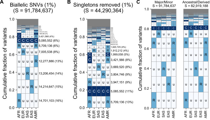
Figure 3. A summary of geographic distributions in human SNVs.

(A) We observe variants at ~3.1% of the measurable sites in the reference human genome (GRCh38). A measurable site is one at which it is possible to detect variation with current sequencing technologies (currently approximately 2.9 Gb out of 3.1 Gb in the human genome; ). (B and C) The relative abundance of different geographic distributions for 1KGP variants, (B) including singletons, and (C) excluding singletons. In panels B and C, the right-hand rectangles show the number and percentage of variants that fall within the corresponding geographic code on the left-hand side; distribution patterns are sorted by their abundance, from bottom-to-top. See Figure 2 for an explanation of the five-letter ‘u’, ’R’, ’C’ codes. The proportion of the genome with variants that have a given geographic distribution code can be calculated from the data above (for example, with the ‘Ruuuu’ code, as 17% × 3.1% = 0.53%). The gray box represents geographic distribution codes whose abundances are too rare to effectively display at the given figure resolution.

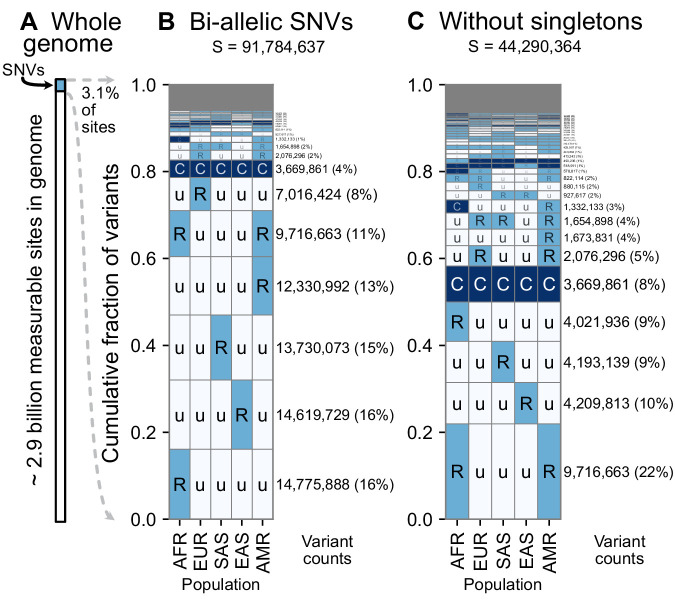
Figure 3.

Figure 3—figure supplement 1. Alternate versions of the GeoVar plots with an alternateallele frequency threshold and tracking derived versus minor allele frequencies.

Figure 3—figure supplement 1.

(A) The relative abundance of geographic distribution codes within the ~92 million variants when using an MAF of 1% as the distinction between ‘common’ (‘C’), and ‘rare’ (‘R’). The right-hand panel shows the percentage of variants that fall within the geographic code represented on the left-hand side; distribution patterns are sorted by their abundance, from bottom-to-top. (B) The abundance of geographic distribution codes for ~44 million non-singleton variants using an MAF of 1% as the boundary between ‘common’ (‘C’), and ‘rare’ (‘R’). (C) Comparison for the abundance of geographic distribution codes when polarizing to the ancestral and derived allele (using build 38) versus major/minor allele. We only include positions where an ancestral allele is supported by at least two outgroups. At 96.6% of variants (80,068,013/82,919,198), the minor allele is also the derived allele. Human ancestral allele calls for GRCh38 based on an eight primate EPO alignment from Ensembl (see key resources table), using only ancestral allele calls supported by at least two outgroup species.

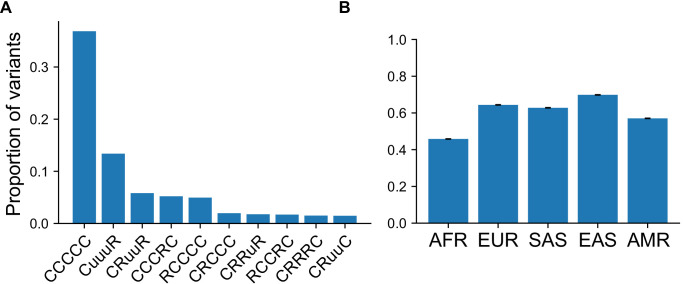
Figure 3—figure supplement 2. Proportion of variants with specific GeoVar patterns conditional on an allele being common in at least one continental group.

Figure 3—figure supplement 2.

(A) Top 10 categories when conditioning on the variant being ‘common’ (MAF >5%) in at least one continental group. Conditioned on a variant being common in a single g, 37.3% of variants are categorized as ‘globally common’ or ‘CCCCC’. (B) The proportion of variants that fall within the ‘globally common’ or ‘CCCCC’ geographic distribution code conditional on the variant being common (MAF >5%) in the specific continental group.

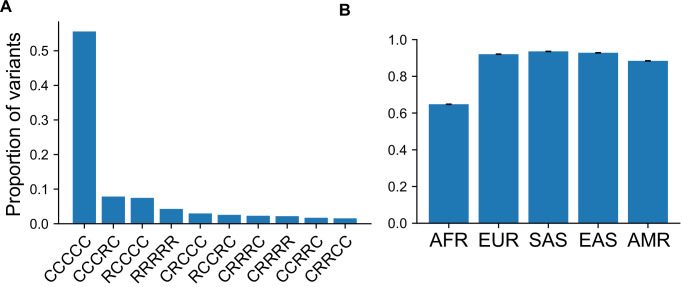
Figure 3—figure supplement 3. Proportion of variants with specific GeoVar patterns conditional on an allele being `globally widespread'.

Figure 3—figure supplement 3.

(A) The proportion of variants that fall within a given geographic distribution code conditional on the variant being ‘globally widespread’, that is, a category that has no unobserved ('u') codes. We note that 55.6% of variants conditioned on being globally widespread are also globally common (‘CCCCC’). In terms of absolute numbers, variants that are common in at least one population (S = 9,958,838) that are also globally widespread (S = 6,322,767) comprise ~63% of the total when conditioning on being common in at least one population. When conditioning on variants common only in regions outside Africa (S = 7,544,648), the percentage of globally widespread variants (S = 6,179,781) increases to ~82%. (B) The proportion of variants that fall within a ‘globally present’ category, defined as categories that contain no unobserved (‘u’) codes, conditional on the variant being common (MAF >5%) in the specific continental group.

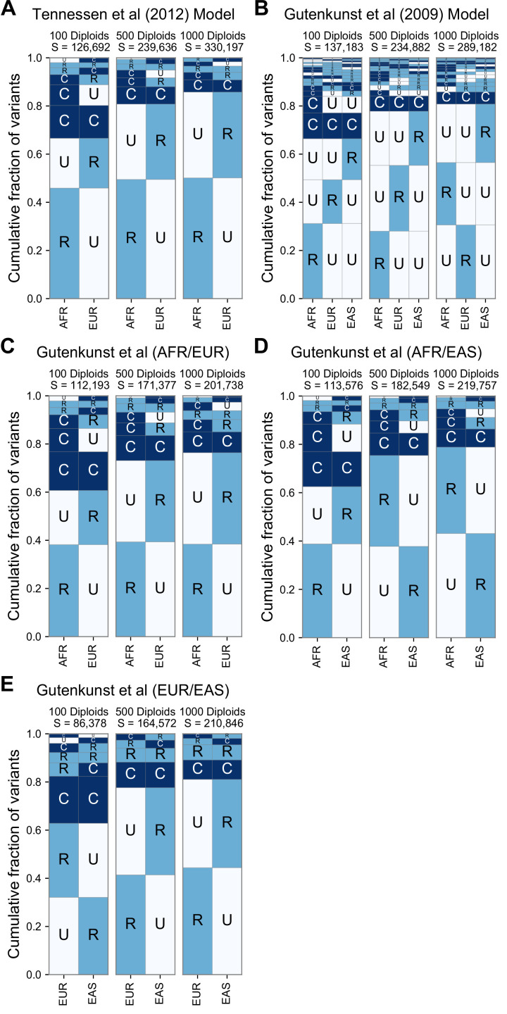
Figure 3—figure supplement 4. GeoVar plots derived from simulations of two published models of human demography.

Figure 3—figure supplement 4.

(A) Gutenkunst et al., 2009, (B–E) Tennessen et al., 2012. For each model, we used stdpopsim (Adrion et al., 2020) to simulate 10 replicates of SNVs equivalent to 5% of Chromosome 22. For each model we simulated three different sample sizes per population, the first with 100 diploid samples, 500 diploid samples, and 1000 diploid samples. The panels with n = 500 diploid samples per population most closely match the sampling within the 1KGP (nAFR = 504, nEUR = 503, nEAS = 504). Both models replicate the qualitative prevalence of the ‘localized rare’ (‘RU’) and ‘globally common’ (‘CC’) patterns that we see in the 1KGP data. With higher sample sizes we find an increased proportion of localized rare (‘RU’) patterns, due to increased detection power. Panels (C–E) show specific pairwise comparisons of populations in the model of Gutenkunst et al., 2009 to compare against the two-population model of Tennessen et al., 2012. Panels (A) and (C) show that, when restricted to AFR/EUR comparisons, the two models predict very similar patterns. The prevalence of localized rare and globally common patterns is reproduced across all comparisons, as is the dependence on sample size. The EUR/EAS comparison (E) shows a larger number of ‘RR’ patterns, presumably reflecting the more recent divergence of those populations.