Identifying Centromeric RNAs Involved in Histone Dynamics In Vivo

Abstract

Over the last decade, the long accepted dogma that heterochromatin is silent has been challenged by increasing evidence of active transcription in these apocryphally annotated quiescent regions of the genome. The recent discovery of noncoding RNAs (ncRNAs) originating from, or localizing to, centromeres, pericentromeres, and telomeres (ie, constitutive heterochromatin) suggest a potential role for ncRNAs in genome integrity. This new paradigm suggests that ncRNAs may recruit chromatin-binding factors, stabilize the higher order folded state of the chromatin fiber, and participate in regulation of processes such as transcription-mediated nucleosome assembly. Thus, identifying, purifying, and elucidating the function of ncRNAs has the potential to provide key insights into genome organization and is currently a topic of intense experimental investigation.

1. INTRODUCTION

Constitutive heterochromatin, including centromeres, pericentromeres, and telomeres, forms condensed chromatin structure and is associated with transcriptional silencing. In humans, centromeres consist of AT-rich 171 bp α-satellite repeats lacking any known genes (Miga, 2015; Waye & Willard, 1987). This alpha-satellite repeat sequence is not conserved across species; however, centromeres do play a conserved function in guiding correct chromosome segregation during mitosis, suggesting an epigenetic basis for centromere identity (Verdaasdonk & Bloom, 2011). Despite the heterogeneity of α-satellite repeats, recent studies suggest that transcription at centromeres is essential for maintaining centromere structure and function (Chan & Wong, 2012; Hall, Mitchell, & O’Neill, 2012).

In a recent study, we reported on a potential role for cell-cycle specific centromeric transcription and the resulting transcripts in the maintenance of centromere integrity in HeLa cells (Quenet & Dalal, 2014). Our data supported the hypothesis that centromeric noncoding RNAs (ncRNAs) may be involved in the targeting of centromeric factors to the centromere, including the histone variant CENP-A. By their nature, centromeric transcripts are presumed to be repetitive, and consequently may originate from regions underrepresented in their entirety in the current database of the human genome project (http://www.ncbi.nlm.nih.gov/genome/guide/human/). Therefore, we adapted protocols described in the literature to better characterize centromeric RNAs. In this chapter, we provide a detailed description of tools currently being used by others and us, in the investigation of ncRNAs associated with chromatin from cultured cells. We also include suggestions for controls, as well as cautionary notes for the interpretation of data generated by such studies. In Sections 3.2 and 3.3, we describe strategies for performing chromatin-associated RNA immunoprecipitation sequencing (RIP-Seq) and immunofluorescence/RNA FISH. In Section 3.4, we discuss bioinformatics approaches to analyze RIP-Seq data.

2. MATERIALS

RNAs are easily deteriorated by nucleases and heat. To protect samples from degradation, extremely cautious laboratory practices are essential, including a dedicated “RNA” bench decontaminated with nuclease-inhibitor solutions like RNase AWAY (#10328-011, Thermo Fisher Scientific/Ambion, Grand Island, NY) or equivalent, wearing clean gloves and lab coat, and covering up hair if necessary. Buffers must be prepared fresh with pure and nuclease-free reagents in nuclease-free reaction tubes using decontaminated pipettes and nuclease-free filter tips. Samples must be kept at 4°C or on ice as much as possible.

2.1. Tissue Cell Culture Elements

• 2.1.1.Human HeLa cell line (ATCC^®, Manassas, VA).
• 2.1.2.10 × Phosphate-buffered saline, pH 7.4 (PBS, #70011-044, Thermo Fisher Scientific/Gibco, Grand Island, NY).
• 2.1.3.Trypsin (#25300, Thermo Fisher Scientific/Gibco).
• 2.1.4.Cell growth medium: Dulbecco/Vogt modified Eagle’s minimal essential medium (DMEM, #11995-081, Thermo Fisher Scientific/Gibco); 10% fetal bovine serum (FBS, #10437-028, Thermo Fisher Scientific/Gibco); and 1% penicillin/streptomycin (#15140-163, Thermo Fisher Scientific/Gibco).

2.2. RNA Immunoprecipitation Components

• 2.2.1.1 × PBS; 0.1% Tween^® 20 (#P2287, Sigma-Aldrich, St Louis, MO).
• 2.2.2.Formaldehyde (#15680, Electron Microscopy Sciences, Hatfield, PA).
• 2.2.3.Glycine (#50046, Sigma-Aldrich).

  Note: A 1 M solution is prepared in RNase–DNase free water (#AM9932, Thermo Fisher Scientific/Ambion), filtered under a tissue culture hood using a 50 mL sterile filter unit (#09-741-88, Nalgene, Cleveland, OH), and stored at 4°C.

• 2.2.4.TM2: 20 mM Tris–HCl, pH 8.0 (#15568-025, Thermo Fisher Scientific); 2 mM magnesium chloride (MgCl2, #AM9530G, Thermo Fisher Scientific); 0.5 mM phenylmethylsulfonyl fluoride (PMSF, #78830, Sigma-Aldrich); 1 × complete protease inhibitor cocktail (#05892953001, Roche, Indianapolis, IN).

  Note: A 200 mM stock solution of PMSF diluted in ethanol is prepared in advance and stored at −20°C.

  Note: A 50 × stock solution of complete protease inhibitor cocktail is prepared by dissolving one tablet in 1 mL RNase–DNase free water and stored for up to 12 weeks at −20°C.

• 2.2.5.TM2±0.5%Nonidet™P 40 Substitute (#74385, Sigma-Aldrich).
• 2.2.6.Ribonucleoside Vanadyl Complex (RVC, #1402, New England Biolabs—NEB, Ipswich, MA).

  Note: RVC or other RNase inhibitor is used in order to avoid RNA degradation. RVC is added in buffers which do not contained ethylenediaminetetraacetic acid (EDTA) or ethylene glycol tetraacetic acid (EGTA) (eg, TM2), as they have the property to dissociate and inactivate the complex.

• 2.2.7.TE: 0.1 M sodium chloride (NaCl, #24740-011, Thermo Fisher Scientific); 10 mM Tris–HCl, pH 8.0; 0.2 mM EGTA (#03777, Sigma-Aldrich).

  Note: A 0.5 M stock solution of EGTA (pH 7.5) is prepared in RNase–DNase free water, filtered under a tissue culture hood using a 50 mL sterile filter unit, and stored at room temperature.

• 2.2.8.Micrococcal Nuclease (MNase, #N3755, Sigma-Aldrich).

  Note: A stock solution at 0.5 unit/μL is prepared in 10 mM Tris–HCl, 50 mM NaCl, 1 mM EDTA, 50% glycerol, aliquoted, and stored at −20°C. Thawed aliquot is kept at 4°C for up to 1 week.

• 2.2.9.CaCl₂ (#746495, Sigma-Aldrich).

  Note: A 100 mM stock solution of CaCl₂ is prepared in RNase–DNase free water, filtered under a tissue culture hood using a 50 mL sterile filter unit, and stored at room temperature.

• 2.2.10.

  EGTA (see step 2.2.7).

• 2.2.11.

  Low-salt buffer: 0.5 × PBS, 5 mM EGTA, 0.5 mM PMSF, 1 × complete protease inhibitor cocktail.

• 2.2.12.

  Murine RNase inhibitor (#M0314S, NEB).

  Note: Murine RNase inhibitor is a replacement for RVC in buffers containing EDTA or EGTA (eg, low-salt buffer).

• 2.2.13.

  Protein A/G PLUS agarose beads (#sc-2003, Santa Cruz Biotechnology, Dallas, TX).

• 2.2.14.

  Anti-CENP-A antibody (#ab13939, Abcam, Cambridge, MA).

• 2.2.15.

  Elution buffer: 1% sodium dodecyl sulfate (SDS); 0.1 M sodium bicarbonate (NaHCO₃, #S6014, Sigma-Aldrich).

  Note: A 1 Mstock solution of NaHCO₃ is prepared in RNase–DNase free water, filtered under a tissue culture hood using a 50 mL sterile filter unit, and stored at room temperature.

• 2.2.16.

  NaCl (#24740-011, Thermo Fisher Scientific).

• 2.2.17.

  Proteinase K (#AM2548, Thermo Fisher Scientific/Ambion).

• 2.2.18.

  Proteinase K buffer: 10 mM Tris–HCl, pH 6.5; 1 mM EDTA.

• 2.2.19.

  DNaseI (RNase free, #AM2222, Thermo Fisher Scientific/Ambion).

• 2.2.20.

  Phenol:chloroform:isoamylalcohol (25:24:1, #77617, Sigma-Aldrich).

• 2.2.21.

  Chloroform (#C7559, Sigma-Aldrich).

• 2.2.22.

  Sodium acetate 3 M, pH 5.2 (#S7899, Sigma-Aldrich).

• 2.2.23.

  Absolute Ethanol (#459844, Sigma-Aldrich).

2.3. Immunofluorescence/RNA FISH Buffers

• 2.3.1.HANKS buffer (#14170112, Thermo Fisher Scientific).
• 2.3.2.Fixation solution: 4% Paraformaldehyde (#15714, Electron Microscopy Sciences); 1 × PBS; RNase–DNase free water.
• 2.3.3.1 × PBS (#10010-023, Thermo Fisher Scientific).
• 2.3.4.Permeabilization solution: 0.1% Triton X-100 (#T8787, Sigma-Aldrich); 1 × PBS.
• 2.3.5.IF buffer: 1 × PBS; 1% normal goat serum (#005-000-121, Jackson ImmunoResearch, West Grove, PA); 50 units of murine RNase inhibitor (see Section 2.2; step 2.2.12).
• 2.3.6.Anti-CENP-A antibody (#ab13939, Abcam, Cambridge, MA).
• 2.3.7.Goat anti-Mouse IgG (H+L) secondary antibody, Alexa Fluor^® 488 conjugate (#A-11001, Thermo Fisher Scientific).
• 2.3.8.RNase A (#12091-021, Thermo Fisher Scientific).
• 2.3.9.Wash solution A: 2 × saline-sodium citrate buffer (SSC, #AM9763, Thermo Fisher Scientific/Ambion); 10% deionized formamide (# 15745, Electron Microscopy Sciences); RNase–DNase free water.

  Note: Deionized formamide has to be stored at 4°C. Before using it, let the solution warm up at room temperature.

• 2.3.10.

  Hybridization solution: 10% dextran sulfate (w:v, #S4030, EMD Millipore, Billerica, MA), 2 × SSC nuclease-free, 10% deionized formamide, RNase–DNase free water.

  Note: For a final volume of 10 mL, 1 g of dextran sulfate is dissolved in 7 mL of RNase–DNase water on an end-over rotator for 30—60 min. Then, 1 mL of 20 × SSC and 1 mL of deionized formamide are added, and the volume is completed to 10 mL with RNase–DNase free water. Aliquots of 500 μL are stored at −20°C for future use.

• 2.3.11.

  RNA FISH Probes labeled with Quasar dyes (ie, Quasar^®570—Cy3™ Replacement or Quasar^®670—Cy5™ Replacement) (Biosearch Technologies, Petulama, CA).

  Note: The desiccated probe set is redissolved in TE buffer (10 mMTris–HCL, 1 mMEDTA, pH 8.0) to obtain a 25 μMstock solution, aliquoted, and stored at −20°C. A 2.5 μM working solution is prepared by diluting 10 times the stock solution.

  Note: The robustness of RNA FISH depends critically on probe quality. Several companies offer access to software which can automatically design probes specifically recognizing a transcript of interest (Baker, 2012). For our assays, we used RNA FISH Probes designed by LGC Biosearch Technologies’ Stellaris RNA FISH Probe Designer (https://www.biosearchtech.com/support/tools/design-software/stellaris-probe-designer). Probe sets can contain up to 48 labeled oligonucleotides modified with a single fluorophore. The probe set targeting the consensus centromeric sequence (ie, α-satellite repeats) was designed against the 171-bases consensus sequence first described by Waye and Willard (1987). The short α-satellite sequence allows the generation of only 11 probes (5′-gcacacatcacaaagaagtt-3; 5′-ggttcaactctgtgagttga-3′; 5′-gagtgtttcaaaactgctct-3′; 5′-caaagcgctccaaatatcca-3′; 5′-agatattccgtttccaacga-3′; 5′-gagaatgcttctgtctagtt-3′; 5′-gcacacatcacaaagaagtt-3′; 5′-ggttcaactctgtgagttga-3′; 5′-gagtgtttcaaaactgctct-3′; 5′-caaagcgctccaaatatcca-3′; 5′-agatattccgtttccaacga-3′). Chosen control probe set targets human NEAT1 (#SMF-2036-1, Biosearch Technologies).

• 2.3.12.

  Hybridization mix: 50 μL of hybridization solution; 2 μL of 2.5 μM probe set (per 18 mm coverslip).

  Note: No competitor DNA (eg, sheared salmon sperm DNA, human Cot1, Escherichia coli tRNA) was added to the hybridization mix. Competitor DNA is used primarily to decrease background and reduce binding of probes to nonspecific loci. However, if the hybridization is limited to 4 h, these potential issues can be limited. If desired, add 5 μg of sheared salmon sperm DNA and 5 μg of E. coli tRNA to the hybridization mix per slide.

• 2.3.13.

  Wash solution B: 2 × SSC; RNase–DNase free water.

• 2.3.14.

  Antifade mounting medium Prolong Gold with DAPI (#P36935, Thermo Fisher Scientific).

3. METHODS

3.1. Tissue Cell Culture: Maintenance of HeLa Cells

HeLa cells are typically harvested twice a week, and a new F175 flask is prepared to maintain the cell line at each passage. Passage numbers should be noted for replicate experiments regardless of which cells in culture are used.

• 3.1.1.Wash cells two times with sterile 1 × PBS.
• 3.1.2.Incubate for 2–3 min at 37°C with 1 mL of 0.05% trypsin, or until cells start to be round.

  Note: Check under an inverted microscope every minute to assess the extent of cell trypsinization. A long incubation or presence of high levels of trypsin can damage cell membrane, leading to cell death and potential artifacts.

• 3.1.3.Stop trypsin activity by addition of 10 volumes of cell growth medium.
• 3.1.4.Resuspend cells very gently, pipetting up and down using a cut-off pipet tip.
• 3.1.5.Transfer 1 mL of trypsinized cells in a new F175 flask containing 19 mL of cell growth medium.
• 3.1.6.Mix gently.
• 3.1.7.Incubate in CO₂ incubator (37°C, 5% CO₂, high relative humidity level).

3.2. RIP-Seq

This protocol was previously described in Quenet and Dalal (2014). Notes are added below to discuss steps that can be modified or where caution should be used.

Day 1

• 3.2.1.Spread cells in F175 flask using the same protocol as described in Section 3.1.

  Note: Five F175 flasks at a final confluency of 80% are used per RIP-Seq. The number of flasks depends on the abundance of the studied histone variants, the efficacy of the immunoprecipitation and the specificity of the antibody.

Day 2

• 3.2.2.Trypsinize cells with 1 mL trypsin (0.05% final concentration).
• 3.2.3.Wash cells two times with cold 1 × PBS; 0.1% Tween 20.
• 3.2.4.Fix cells with 0.1% formaldehyde for 10 min at room temperature.

  Note: Formaldehyde fixation allows study of direct and indirect bindings. To analyze direct interactions only, UV-crosslinking is preferred (150–200 mJ/cm² at 254 nm using a Stratalinker^® UV crosslinker).

• 3.2.5.Quench by addition of glycine (125 mM final concentration).
• 3.2.6.Wash cells twice with cold 1 × PBS, 0.1% Tween 20. Between washes, collect cells by 5 min centrifugation at 800 rpm at 4°C.

  Note: A low speed of centrifugation is preferred, so as not to damage cells.

• 3.2.7.Isolate nuclei in TM2 buffer complemented with 0.5% Nonidet™ P 40 Substitute and 10 mM of RVC.
• 3.2.8.Wash once with TM2 buffer containing 10 mM of RVC.
• 3.2.9.Collect chromatin by centrifugation at 800 rpm for 5 min at 4°C.
• 3.2.10.

  Digest chromatin with MNase in 0.1 M TE buffer complemented with 2 mM CaCl₂

• 3.2.11.

  Stop the MNase action by addition of 10 mM EGTA and transfer on ice.

  Note: The time of incubation and the MNase concentration depends on the desired size of the chromatin array. In our hands, 2 min and 8 min incubation with 0.2 unit/mL of MNase (Sigma) results in chromatin arrays containing 3–5 and 1–2 nucleosomes, respectively.

• 3.2.12.

  Collect chromatin by gentle centrifugation at 800 rpm for 5 min at 4°C.

  Note: It is critical that all buffers be pure and nuclease/protease free for all subsequent handling of chromatin. Gentle handling of chromatin can reduce degradation and dissociation, which can be monitored by taking a small sample for DNA (agarose gel) and histone (Western blot) analyses respectively, or by analyzing a small portion of the chromatin under an atomic force microscope for “beads on a string” appearance.

• 3.2.13.

  Resuspend the nuclear pellet in 1 mL low-salt buffer complemented with 50 units of murine RNase inhibitor.

  Note: Salt concentration can be increased to a total of 0.35 M NaCl, which will lead to the disassociation of chromatin-binding proteins strongly associated to chromatin, including most linker histone H1 species.

• 3.2.14.

  Extract chromatin overnight at 4°C in an end-over-end rotator.

Day 3

• 3.2.15.

  Centrifuge sample for 5 min at 8000 rpm at 4°C.

• 3.2.16.

  Save an aliquot of the supernatant, and label it “input.”

• 3.2.17.

  Preclear the supernatant with 30 μL of protein A/G Plus agarose beads for 30 min at 4°C in an end-over-end rotator.

  Note: To avoid RNAs and protein degradation, fresh murine RNase inhibitor and complete protease inhibitor cocktail are added at this step.

• 3.2.18.

  Centrifuge at 800 rpm at 4°C for 5 min.

• 3.2.19.

  Incubate the supernatant with the anti-CENP-A (or protein of choice) primary antibody (5 μL for 5 flasks) for a minimum of 4 h and a maximum of 12 h.

  Note: The incubation with the primary antibody can be extended up to a maximum of 12 h, but shorter incubation periods are preferred to minimize background. Incubating fewer than 4 h results in low yields, although this depends on the avidity of the antibody for its epitope in the antigen.

• 3.2.20.

  Immunoprecipitate CENP-A/primary antibody complex with 50 μL of protein A/GPLUS agarose beads for 2 h at 4°C on the end-over-end rotator.

• 3.2.21.

  Centrifuge at 800 rpm at 4°C for 5 min.

• 3.2.22.

  Save an aliquot of the supernatant, label it “unbound.”

• 3.2.23.

  Wash three times CENP-A/primary antibody/beads complex with 1 mL low-salt buffer containing murine RNase inhibitor and complete protease inhibitor cocktail.

  Note: To validate the efficacy of the immunoprecipitation technique and the purification of the protein of interest, Western blot analysis must be performed. For this purpose, samples can be divided into two, if the quantity of material is high enough to perform the protein and RNA study with five F175 flasks. Otherwise the number of initial flasks has to be increased.

  Note: At this point, samples can be stored at −80°C. RNA purification described in the following steps should be performed no later than the following week of the immunoprecipitation to avoid potential degradation.

Day 4

• 3.2.24.

  Elute RNA–protein complex in 250 μL elution buffer two times by incubation in an end-over-end rotator for 15 min at room temperature.

• 3.2.25.

  Denature all samples (input, unbound, and beads) in 200 mMNaCl for 2 h at 65°C.

• 3.2.26.

  Digest proteins with 20 μg of proteinase K in proteinase K buffer at 42°C for 45 min.

• 3.2.27.

  To avoid genomic DNA contamination, treat sample with DNaseI for 30 min at 37°C.

• 3.2.28.

  Stop the reaction by adding 5 mM EDTA.

• 3.2.29.

  Purify RNAs by the phenol:chloroform:isoamylalcohol method.

  Note: Mix equal volume of sample (~500 μL) with phenol: chloroform:isoamylalcohol solution and shake by hand for 1 min. Centrifuge for 15 min at 10,000 rpm at 4°C. Transfer the top aqueous phase to a new tube, mix with equal volume of chloroform and hand shake for 1 min. Centrifuge for 15 min at 10,000 rpm at 4°C. Transfer the top aqueous phase to a new tube, add 1/10 volume of sodium acetate (final concentration ~0.3 M) and 3 volumes of absolute ethanol. Incubate at −20°C overnight or −80°C for 30 min. Centrifuge for 30 min at 10,000 rpm at 4°C. Resuspend dry pellet in 30 μL RNase–DNase free water. Samples can be stored at −80°C until further analysis.

• 3.2.30.

  Determine RNA concentration by UV-spectra and quality using a Bioanalyzer instrument (#5067-1511, Agilent Technologies, Santa Clara, CA).

Day 5

• 3.2.31.

  Prepare DNA library and sequence by the Illumina approach or other method of your choice.

  Note: The library was prepared and sequenced using Illumina TruSeq^® Stranded Total RNA Sample Preparation and TruSeq v4 chemistry (Illumina, San Diego, CA).

  Note: An important decision at the library preparation stage is whether enrichment for poly-A transcripts or depletion of ribosomal transcripts is necessary. This choice could greatly increase the final signal-to-noise ratio. Ribosomal transcripts represent the majority of molecules in a total RNA sample, potentially reducing RNA signal (Zhao et al., 2014). However, targeting ncRNA would abrogate the use of oligo-dT beads (ie, ncRNA can either be poly-A or not), and RiboZero depletion may not work efficiently if those transcripts are fragmented by the chromatin-immunoprecipitation protocol. Since a robust and specific immunoprecipitation should effectively purify only targets of interest, ribosomal depletion is commonly not performed. Still, in practice, RIP samples can be composed of up to 90% rRNA (Lu, Guan, Schmidt, & Matera, 2014). The ribosomal component can be estimated before sequencing (Schroeder et al., 2006). Once a library is sequenced, ribosomal reads can also be easily removed computationally post hoc. The protocol described in Section 3.4 presents this approach.

• 3.2.32.

  Analysis of data (see Section 3.4).

  Note: Since nucleic acids can bind to various surfaces, we suggest including a number of controls:

  1. Testing the specificity of each new lot of antibody (confirm by Western blot or mass spectrometry that the protein of choice is the primary captured target);
  2. Using a heterologous protein to ensure specificity of identified RNAs bound to the protein of interest;
  3. Including mock immunoprecipitation with beads alone or IgG immunoprecipitation;
  4. Performing at least two (preferably more) biological replicates spread out over the course of a few months to sample cell passage numbers;
  5. Where possible, performing the “gold standard” test, namely, depleting the protein of interest to ensure that any RNAs identified in the subsequent RIP-Seq are specific to that protein, and do not bind indiscriminately to the antibody or beads;
  6. Confirming the localization at the same locus by an alternative approach, like RNA FISH coupled to immunofluorescence (see Section 3.3);
  7. Analyzing functional consequences of the downregulation of identified ncRNAs with a focus on the heterochromatic domain of interest (eg, centromeres for CENP-A).

3.3. Immunofluorescence/RNA FISH

The goal of RNA FISH is to visualize the localization of centromeric RNAs in human cells. In order to define their subnuclear localization, the RNA signal can be compared to the localization of proteins of interest, like centromeric proteins, by an experiment of immunofluorescence combined to RNA FISH (IF/RNA FISH).

Several published protocols were tested (eg, combined immunofluorescence/RNAFISH described by Chaumeil et al., and simultaneous immunofluorescence/RNAFISH described in Raj et al. (Chaumeil, Augui, Chow, & Heard, 2008; Raj, van den Bogaard, Rifkin, van Oudenaarden, & Tyagi, 2008)). For centromeric ncRNA detection, the clearest and most reproducible results were obtained from the following modified protocol of sequential immunofluorescence/RNA FISH from Raj et al. (2008).

Day 1

• 3.3.1.Spread cells on poly-L lysine coverslip in 6-well plate at ~75% confluency using the same protocol than described in Section 3.1.

Day 2

• 3.3.2.Wash cells three times with HANKS buffer.
• 3.3.3.Fix cells with the fixation solution for 10 min at room temperature.
• 3.3.4.Wash out fixation solution with 1 × PBS for 5 min two times at room temperature.
• 3.3.5.Permeabilize cells for 5 min at room temperature.
• 3.3.6.Wash coverslip with 1 × PBS for 5 min at room temperature.
• 3.3.7.Incubate with diluted anti-CENP-A primary antibody (d = 1/20,000) in IF buffer overnight at 4°C.

  Note: Several kinetochore proteins are present at human centromeres all over cell cycle. Consequently, other kinetochore proteins can be stained, such as CENP-B (dilution 1/400, Anti-CENP-B antibody, #ab25734, Abcam).

• 3.3.8.Wash cells with 1 × PBS for 10 min at room temperature three times.
• 3.3.9.Incubate with secondary antibody (d = 1/750) in IF buffer for 1 h at room temperature in the dark.
• 3.3.10.

  Wash with 1 × PBS for 10 min at room temperature in the dark three times.

  Note: At this step, a couple of slides can be washed with 1 × PBS complemented with 1 mg/mL of RNase A, to run out potentially nonspecific recognition of the probe set with DNA. It is essential to separate RNase A treated coverslips from RNase A not treated coverslips, to avoid contamination, by using two sets of 6-well plates and pipettes.

• 3.3.11.

  Fix with the fixation solution for 10 min at room temperature in the dark.

• 3.3.12.

  Wash twice with 1 × PBS for 10 min at room temperature in the dark.

• 3.3.13.

  Wash with wash solution A for 5 min at room temperature in the dark.

• 3.3.14.

  Incubate with hybridization mix for 4 h at 37°C in the dark.

  Note: Hybridization can proceed for up to 16 h, however, with increasing risk of higher background, nonspecific binding, and RNA degradation.

  Note: Keeping the coverslips in a humidified atmosphere is essential for the efficacy of the hybridization. Several options exist to achieve this, including the use of Petri dish sealed twice with parafilm “M” and containing a wet tissue. Additionally, hybridization is performed on parafilm “M” with cells facing down to assure the equal hybridization mix on the surface of the coverslip and avoid bubbles.

  Note: It is crucial to set the temperature of the incubator/hybridization oven at precisely 37°C. Any change (lower or higher) will affect the efficiency of the hybridization.

• 3.3.15.

  Wash twice with wash solution A for 30 min at 37°C in the dark.

  Note: Wash solution A needs to be warmed up before use.

• 3.3.16.

  Wash with solution B for 5 min at room temperature in the dark.

• 3.3.17.

  Mount coverslips onto the slide with Prolong Gold or other mounting medium containing DAPI.

  Note: Slides can be kept at room temperature for up to 1 h and then stored at 4°C.

• 3.3.18.

  Acquire and analyze pictures in the following 3 days.

  Note: Slides were observed with a DeltaVision RT microscopy imaging system (GE Healthcare, Pittsburgh, PA) controlling an interline charge-coupled device camera (Coolsnap, Tucson, AZ) mounted on an inverted microscope (IX-70; Olympus, Center Valley, PA). Images were captured by using a 60 × objective at 0.2 μm z-sections and analyzed with Image J (1.50e; Java 1.6.0_20, NIH, Bethesda, MD). One z-stack is represented in Figs. 1 and 2.

Fig. 1.

Control immunofluorescence/RNA FISH on nonsynchronized HeLa cells. CENP-A protein is stained by immunofluorescence, followed by NEAT1 RNA hybridization. Bottom panels present cells treated with RNase A prior to RNA FISH. Only one z-stack is shown. Scale bar represents 10 μm.

Fig. 2.

Immunofluorescence/RNA FISH on nonsynchronized HeLa cells. CENP-A protein is stained by immunofluorescence, followed by α-satellite RNA hybridization. Bottom panels present cells treated with RNase A prior to RNA FISH. Only one z-stack is shown. Scale bar represents 10 μm.

3.4. Computational Analysis

Although a standardized unified method for RIP-Seq analysis is currently lacking, one can treat RIP-Seq data similarly to RNA-Seq or ChIP-Seq data, which have more well-established tools. The former approach aims to identify and quantify transcripts that are associated with your protein of interest. The latter is a peak-calling approach that identifies a genomic region and indirectly identifies the originating transcript (Zambelli & Pavesi, 2015). This chapter will focus primarily on the former approach.

The overall analysis strategy is presented in Fig. 3. Individual steps labeled in this figure are described later.

Fig. 3.

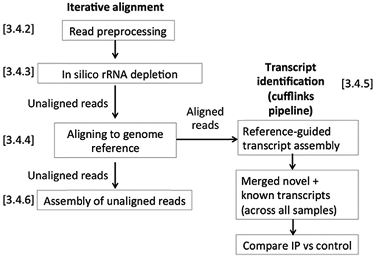
Example of RIP-Seq analysis pipeline.

3.4.1. Sequencing Strategy

The sequencing strategy for the RIP-Seq experiment involves settling the read length and depth for studied samples. These decisions are important to maximize the inferences you can make about the source molecules in your original pool. For RIP-Seq, the strategy should be similar to an RNA-Seq experiment, with long paired end reads. In the example dataset for which this protocol was developed, libraries were sequenced on an Illumina HiSeq 2500 in paired end mode for 125 cycles for each end, using Illumina TruSeq v4 chemistry. To analyze the outcome, reads are aligned to a genomic reference following a multistep process described in Sections 3.4.2-3.4.4.

Note: The choice of sequencing depth is based on the complexity of the library you wish to sequence, the enrichment you hope to obtain, the amount of replication you will perform, and cost of the experiment (Sims, Sudbery, Ilott, Heger, & Ponting, 2014). Early ENCODE guidelines for ChIP-Seq of “point source” peaks, such as transcription factors, suggest a modest requirement of 10 million uniquely mapped reads per experiment to find enriched regions (Landt et al., 2012). For RNA-Seq, 30 million reads is an often-cited minimum for mammalian gene expression profiling, with 100 million needed for novel isoform discovery, and >200 million for saturated detection (Sims et al., 2014). For RIP-Seq experiments, where a less diverse set of transcript molecules is expected to be sequenced, 20 million reads is a reasonable minimum for a protein with a small number of expected targets.

3.4.2. Read Preprocessing

Reads should be preprocessed to remove errors and artifacts that could lead to inaccurate mapping. Raw reads commonly display systematic errors, including reduced base-calling accuracy and adapter sequence contamination. A first pass quality assessment can help identify these systematic errors. An effective tool to achieve this is FastQC (Simon Andrews, http://www.bioinformatics.babraham.ac.uk/projects/fastqc/). This tool provides several graphical results including base-calling quality by position, base composition, and overrepresented sequences, which allow the identification of adapter contamination or other types of error.

Once the error profile is established, a read preprocessing strategy is chosen that preserves read length while maximizing alignability. The two major options are adaptive trimming, where each read is processed individually and trimmed to variable lengths; or fixed cropping, where an equal number of bases is trimmed from each read. Unless the read mapping percentage is very low (<75%), fixed cropping is recommended as it provides the maximum compatibility with downstream analysis tools (ie, some count-based algorithms assume all reads are of equal length, such as MISO (Katz, Wang, Airoldi, & Burge, 2010)). We used the Trimmomatic tool that can perform either strategy (Bolger, Lohse, & Usadel, 2014). Preprocessed reads were then further refined in order to deplete ribosomal RNA (rRNA).

3.4.3. In Silico rRNA Depletion

Immunoprecipitated samples may include a significant fraction of rRNA transcripts, which are not the binding partners of interest, particularly if no oligo-dT selection or ribosomal depletion is performed. The proportion of rRNA can vary between experiments, leading to the spurious detection of novel transcripts and inaccurate abundance estimations when transcript abundances are normalized by total depth. In silico rRNA depletion mitigates these problems.

In silico rRNA depletion consists of aligning reads to a reference of rDNA sequence and extracting the unaligned reads for downstream analysis. There are many alignment algorithms available to perform this step (Fonseca, Rung, Brazma, & Marioni, 2012). The most frequently cited are the TopHat and Bowtie programs, which are components of a software suite called the Tuxedo tools (Trapnell et al., 2012). These programs also perform well in systematic comparisons with simulated data (Engstrom et al., 2013). The instructions below perform rRNA depletion using the Bowtie2 aligner (Langmead & Salzberg, 2012):

1. Build a reference database.

   1. Obtain or compile rDNA sequence(s).

      Note: A 43 kb complete rDNA repeating unit in human can be obtained from GenBank (accession U13369.1) in FASTA format.

   2. Using the following command, build a reference database from the rDNA sequence to map reads to:

   bowtie2 index bowtie2-build rDNA.fa rDNA
   

   where “rDNA.fa” contains rDNA sequence in FASTA format. Bowtie2 will compile a set of index files using the prefix “rDNA.”

2. Align reads to the rDNA reference database.

   1. Align preprocessed reads to the rDNA reference.

   2. Save nonmapping reads to a separate file, so that they can be realigned to the genome later (see Section 3.4.4):

   bowtie2 -p 8 -un-concr DNA_unaligned -sensitive -x rDNA \
    - 1 processed_reads_1.fastq.gz -2 processed_reads_2.fastq.gz \
    - S rDNA_alignments.sam
   

   where “rDNA_unaligned” is the file name prefix for your rDNA-filtered reads; “rDNA” is the Bowtie2 index from the previous step (ie, Section 3.4.3.i.b); “processed_reads_x.fastq.gz” is the RIP-Seq reads; and “rDNA_alignments. sam” is the destination file for the alignments to the rDNA sequence.

   Note: A similar strategy was recently described by Miga et al. to reduce the number of false positive alignments with an expanded set of repetitive and “blacklisted” regions (Miga, Eisenhart, & Kent, 2015).

3.4.4. Aligning to a Reference Genome

To determine the origin of transcript molecules from the rDNA-filtered reads, they must be aligned to the complete reference genome. Since reads likely derive from processed spliced transcripts, alignments to the genomic reference may be split to indicate removed introns. The TopHat alignment program performs splice-aware read mapping, producing spliced alignments over splice junctions (Kim et al., 2013). This tool performs alignments to transcript sequence first, and then to genomic DNA. To do this, transcript models must be formatted in gene transfer format (GTF) with chromosome nomenclature consistent with the genomic sequence. To ensure these components are correctly arranged, standardized reference sequences and annotations used to perform the alignment are compiled in a collection called iGenomes (Illumina, https://support.illumina.com/sequencing/sequencing_software/igenome.html). Genome sequence can be obtained from this source as a preformatted index for use with Bowtie2. Once the appropriate reference (ie, the human genome in our study) is downloaded and saved to the proper location, the following command is applied to align reads to the human genome and find splice junctions:

tophat - G genes.gtf -g 1 GRCh38.p2.genome \
   rDNA_unaligned.1 rDNA_unaligned.2

where “genes.gtf” contains transcript coordinates; “GRCh38.p2.genome” is the Bowtie2 index for the build 38 genome sequence; and “rDNA_unaligned.1” and “rDNA_unaligned.2” are the rDNA filtered reads. By default, results will be saved into a folder called “tophat_out.” This can be changed with the “—output-dir” option.

Note: Handling read alignments that map to more than one location in the genome is an important parameter to set. For example, paralogs are genes with a common evolutionary origin that are similar in sequence, such that they may not be uniquely mappable. For accurate transcriptional profiling in paralogs, it is appropriate to allow multiple alignments for a single read. For RIP-Seq application, the more conservative setting of “-g 1” limits alignments to only a single location. This is recommended to limit detection of spurious transcripts from repetitive sequence.

Note: Other sources of reference annotation and sequence may be more comprehensive or current than iGenomes, such as Ensembl (Yates, Akanni, et al., 2016) or GENCODE (Harrow et al., 2012). Additionally, cell line specific assemblies may be used for mapping to avoid errors from polymorphisms and structural variants. In these cases, follow the instructions in Section 3.4.3.i.b. to generate a Bowtie2 index from your sequence. To find out what has changed with successive assembly versions, a useful resource is the Genome Reference Consortium (GRC, http://www.ncbi.nlm.nih.gov/projects/genome/assembly/grc/human/).

3.4.5. Transcript Abundance Estimation

To identify enrichment within the RIP sample relative to control, the abundances of the transcripts need to be estimated. For this purpose, the alignments generated in the previous step (ie, Section 3.4.4) are used to reconstruct the transcript molecules that were present in the original sample and estimate their abundances. The Cufflinks program includes algorithms for performing both of these tasks (Trapnell et al., 2012).

Transcript abundance is calculated in units of fragments per kilobase of transcript per million mapped reads (FPKM), which normalize for sequencing depth and transcript length. A significantly higher FPKM in the RIP sample relative to input or control is evidence of enrichment of the target by immunoprecipitation.

This command compares transcript abundances between an immunoprecipitation and control sample:

cuffdiff -o cuffdiff_out genes.gtf - L IP,Cntrl \
   rip_alignments.bam input_alignments.bam

where “cuffdiff_out” is the name of an output directory; “IP,Cntrl” are labels to identify the immunoprecipitation and control samples in the results; and “rip_alignments.bam” and “input_alignments.bam” are the alignment files (from Section 3.4.4).

Note: The “genes.gtf” can be a reference annotation or de novo assembled transcripts (Trapnell et al., 2012). The latter is preferred if putative targets are unannotated or unknown.

3.4.6. Assembly of Unaligned Reads

The human genome is incompletely sequenced and assembled, particularly within centromeres and heterochromatic regions (Miga, 2015). Even though the most recent reference adds megabases of new centromeric DNA and alternative loci (Rosenbloom et al., 2015), transcript sequence purified by chromatin-immunoprecipitation can still be unalignable to the reference. These unalignable reads may derive from unassembled human genome sequence, or from other sources such as technical artifacts and contaminants. To investigate the source of unaligned reads, they can be assembled into longer fragments. For this purpose, the bam2fastq program (http://gsl.hudsonalpha.org/information/software/bam2fastq) is used to extract unaligned reads from TopHat results (Section 3.4.4) following this command:

bam2fastq -no-aligned -o top_unaligned#.txt unmapped.bam

where “top_unaligned_#.txt” is the name given to the result file, and “unmapped. bam” is the file where TopHat stores the unmapped reads. The pound sign will be replaced with the mate pair number (1 or 2).

Then, reads are assembled in a two-step process using the Velvet program (Zerbino & Birney, 2008):

1. Step of hashing:

   velvethmysteryseqs 21 -fastq -short -separate \
      top_unaligned_1.txt top_unaligned_2.txt >& out1
   

2. Step of contig assembly:

   velvetg mystery1 -min_contig_lgth 150 -ins_length 50
   

   where “mysteryseqs” is your output directory, and the “contig_lgth” and “ins_length” are estimates based on the sequenced fragment length.

The remaining contigs can be mined for additional evidence of transcripts, using BLAST. In the case of contaminants, BLAST will identify significant similarity to bacterial DNA and vector sequence. For technical artifacts, the FastQC program can be used to identify adapter sequence (see Section 3.4.2). Any remaining high-abundance contigs can be mined for evidence of human transcriptional origin or analyzed via RNA FISH (see Section 3.3).

REFERENCES

- Baker M (2012). RNA imaging in situ. Nature Methods, 9, 787–790. [Google Scholar]
- Bolger AM, Lohse M, & Usadel B (2014). Trimmomatic: A flexible trimmer for illumina sequence data. Bioinformatics (Oxford, England), 30, 2114–2120. [DOI] [PMC free article] [PubMed] [Google Scholar]
- Chan FL, & Wong LH (2012). Transcription in the maintenance of centromere chromatin identity. Nucleic Acids Research, 40, 11178–11188. [DOI] [PMC free article] [PubMed] [Google Scholar]
- Chaumeil J, Augui S, Chow JC, & Heard E (2008). Combined immunofluorescence, RNA fluorescent in situ hybridization, and DNA fluorescent in situ hybridization to study chromatin changes, transcriptional activity, nuclear organization, and X-chromosome inactivation. Methods in Molecular Biology (Clifton, NJ), 463, 297–308. [DOI] [PubMed] [Google Scholar]
- Engstrom PG, Steijger T, Sipos B, Grant GR, Kahles A, Ratsch G, et al. (2013). Systematic evaluation of spliced alignment programs for RNA-seq data. Nature Methods, 10, 1185–1191. [DOI] [PMC free article] [PubMed] [Google Scholar]
- Fonseca NA, Rung J, Brazma A, & Marioni JC (2012). Tools for mapping high-throughput sequencing data. Bioinformatics (Oxford, England), 28, 3169–3177. [DOI] [PubMed] [Google Scholar]
- Hall LE, Mitchell SE, & O’Neill RJ (2012). Pericentric and centromeric transcription: A perfect balance required. Chromosome Research, 20, 535–546. [DOI] [PubMed] [Google Scholar]
- Harrow J, Frankish A, Gonzalez JM, Tapanari E, Diekhans M, Kokocinski F, et al. (2012). GENCODE: The reference human genome annotation for The ENCODE Project. Genome Research, 22, 1760–1774. [DOI] [PMC free article] [PubMed] [Google Scholar]
- Katz Y, Wang ET, Airoldi EM, & Burge CB (2010). Analysis and design of RNA sequencing experiments for identifying isoform regulation. Nature Methods, 7, 1009–1015. [DOI] [PMC free article] [PubMed] [Google Scholar]
- Kim D, Pertea G, Trapnell C, Pimentel H, Kelley R, & Salzberg SL (2013). Top-Hat2: Accurate alignment of transcriptomes in the presence of insertions, deletions and gene fusions. Genome Biology, 14, R36. [DOI] [PMC free article] [PubMed] [Google Scholar]
- Landt SG, Marinov GK, Kundaje A, Kheradpour P, Pauli F, Batzoglou S, et al. (2012). ChIP-seq guidelines and practices of the ENCODE and modENCODE consortia. Genome Research, 22, 1813–1831. [DOI] [PMC free article] [PubMed] [Google Scholar]
- Langmead B, & Salzberg SL (2012). Fast gapped-read alignment with Bowtie 2. Nature Methods, 9, 357–359. [DOI] [PMC free article] [PubMed] [Google Scholar]
- Lu Z, Guan X, Schmidt CA, & Matera AG (2014). RIP-seq analysis of eukaryotic Sm proteins identifies three major categories of Sm-containing ribonucleoproteins. Genome Biology, 15, R7. [DOI] [PMC free article] [PubMed] [Google Scholar]
- Miga KH (2015). Completing the human genome: The progress and challenge of satellite DNA assembly. Chromosome Research, 23, 421–426. [DOI] [PubMed] [Google Scholar]
- Miga KH, Eisenhart C, & Kent WJ (2015). Utilizing mapping targets of sequences underrepresented in the reference assembly to reduce false positive alignments. Nucleic Acids Research, 43, e133. [DOI] [PMC free article] [PubMed] [Google Scholar]
- Quenet D, & Dalal Y (2014). A long non-coding RNA is required for targeting centromeric protein A to the human centromere. eLife, 3, e03254. [DOI] [PMC free article] [PubMed] [Google Scholar]
- Raj A, van den Bogaard P, Rifkin SA, van Oudenaarden A, & Tyagi S (2008). Imaging individual mRNA molecules using multiple singly labeled probes. Nature Methods, 5, 877–879. [DOI] [PMC free article] [PubMed] [Google Scholar]
- Rosenbloom KR, Armstrong J, Barber GP, Casper J, Clawson H, Diekhans M, et al. (2015). The UCSC Genome Browser database: 2015 update. Nucleic Acids Research, 43, D670–D681. [DOI] [PMC free article] [PubMed] [Google Scholar]
- Schroeder A, Mueller O, Stocker S, Salowsky R, Leiber M, Gassmann M, et al. (2006). The RIN: An RNA integrity number for assigning integrity values to RNA measurements. BMC Molecular Biology, 7, 3. [DOI] [PMC free article] [PubMed] [Google Scholar]
- Sims D, Sudbery I, Ilott NE, Heger A, & Ponting CP (2014). Sequencing depth and coverage: Key considerations in genomic analyses. Nature Reviews. Genetics, 15, 121–132. [DOI] [PubMed] [Google Scholar]
- Trapnell C, Roberts A, Goff L, Pertea G, Kim D, Kelley DR, et al. (2012). Differential gene and transcript expression analysis of RNA-seq experiments with TopHat and Cufflinks. Nature Protocols, 7, 562–578. [DOI] [PMC free article] [PubMed] [Google Scholar]
- Verdaasdonk JS, & Bloom K (2011). Centromeres: Unique chromatin structures that drive chromosome segregation. Nature Reviews. Molecular Cell Biology, 12, 320–332. [DOI] [PMC free article] [PubMed] [Google Scholar]
- Waye JS, & Willard HF (1987). Nucleotide sequence heterogeneity of alpha satellite repetitive DNA: A survey of alphoid sequences from different human chromosomes. Nucleic Acids Research, 15, 7549–7569. [DOI] [PMC free article] [PubMed] [Google Scholar]
- Yates A, Akanni W, Amode MR, Barrell D, Billis K, Carvalho-Silva D, et al. (2016). Ensembl 2016. Nucleic Acids Research, 44(D1), D710–D716. [DOI] [PMC free article] [PubMed] [Google Scholar]
- Zambelli F, & Pavesi G (2015). RIP-Seq data analysis to determine RNA-protein associations. Methods in Molecular Biology (Clifton, NJ), 1269, 293–303. [DOI] [PubMed] [Google Scholar]
- Zerbino DR, & Birney E (2008). Velvet: Algorithms for de novo short read assembly using de Bruijn graphs. Genome Research, 18, 821–829. [DOI] [PMC free article] [PubMed] [Google Scholar]
- Zhao W, He X, Hoadley KA, Parker JS, Hayes DN, & Perou CM (2014). Comparison of RNA-Seq by poly (A) capture, ribosomal RNA depletion, and DNA microarray for expression profiling. BMC Genomics, 15, 419. [DOI] [PMC free article] [PubMed] [Google Scholar]