COSORE: A community database for continuous soil respiration and other soil‐atmosphere greenhouse gas flux data

Ben Bond‐Lamberty; Danielle S Christianson; Avni Malhotra; Stephanie C Pennington; Debjani Sihi; Amir AghaKouchak; Hassan Anjileli; M Altaf Arain; Juan J Armesto; Samaneh Ashraf; Mioko Ataka; Dennis Baldocchi; Thomas Andrew Black; Nina Buchmann; Mariah S Carbone; Shih‐Chieh Chang; Patrick Crill; Peter S Curtis; Eric A Davidson; Ankur R Desai; John E Drake; Tarek S El‐Madany; Michael Gavazzi; Carolyn‐Monika Görres; Christopher M Gough; Michael Goulden; Jillian Gregg; Omar Gutiérrez del Arroyo; Jin‐Sheng He; Takashi Hirano; Anya Hopple; Holly Hughes; Järvi Järveoja; Rachhpal Jassal; Jinshi Jian; Haiming Kan; Jason Kaye; Yuji Kominami; Naishen Liang; David Lipson; Catriona A Macdonald; Kadmiel Maseyk; Kayla Mathes; Marguerite Mauritz; Melanie A Mayes; Steve McNulty; Guofang Miao; Mirco Migliavacca; Scott Miller; Chelcy F Miniat; Jennifer G Nietz; Mats B Nilsson; Asko Noormets; Hamidreza Norouzi; Christine S O’Connell; Bruce Osborne; Cecilio Oyonarte; Zhuo Pang; Matthias Peichl; Elise Pendall; Jorge F Perez‐Quezada; Claire L Phillips; Richard P Phillips; James W Raich; Alexandre A Renchon; Nadine K Ruehr; Enrique P Sánchez‐Cañete; Matthew Saunders; Kathleen E Savage; Marion Schrumpf; Russell L Scott; Ulli Seibt; Whendee L Silver; Wu Sun; Daphne Szutu; Kentaro Takagi; Masahiro Takagi; Munemasa Teramoto; Mark G Tjoelker; Susan Trumbore; Masahito Ueyama; Rodrigo Vargas; Ruth K Varner; Joseph Verfaillie; Christoph Vogel; Jinsong Wang; Greg Winston; Tana E Wood; Juying Wu; Thomas Wutzler; Jiye Zeng; Tianshan Zha; Quan Zhang; Junliang Zou

doi:10.1111/gcb.15353

. 2020 Oct 7;26(12):7268–7283. doi: 10.1111/gcb.15353

COSORE: A community database for continuous soil respiration and other soil‐atmosphere greenhouse gas flux data

Ben Bond‐Lamberty ^1,^✉, Danielle S Christianson ², Avni Malhotra ³, Stephanie C Pennington ¹, Debjani Sihi ^4,⁷³, Amir AghaKouchak ⁵, Hassan Anjileli ⁵, M Altaf Arain ⁶, Juan J Armesto ^7,⁸, Samaneh Ashraf ⁹, Mioko Ataka ¹⁰, Dennis Baldocchi ¹¹, Thomas Andrew Black ¹², Nina Buchmann ¹³, Mariah S Carbone ¹⁴, Shih‐Chieh Chang ¹⁵, Patrick Crill ¹⁶, Peter S Curtis ¹⁷, Eric A Davidson ¹⁸, Ankur R Desai ¹⁹, John E Drake ²⁰, Tarek S El‐Madany ²¹, Michael Gavazzi ²², Carolyn‐Monika Görres ²³, Christopher M Gough ²⁴, Michael Goulden ²⁵, Jillian Gregg ²⁶, Omar Gutiérrez del Arroyo ¹¹, Jin‐Sheng He ²⁷, Takashi Hirano ²⁸, Anya Hopple ^29,³⁰, Holly Hughes ³¹, Järvi Järveoja ³², Rachhpal Jassal ¹², Jinshi Jian ¹, Haiming Kan ³³, Jason Kaye ³⁴, Yuji Kominami ³⁵, Naishen Liang ³⁶, David Lipson ³⁷, Catriona A Macdonald ³⁸, Kadmiel Maseyk ³⁹, Kayla Mathes ⁴⁰, Marguerite Mauritz ⁴¹, Melanie A Mayes ⁴, Steve McNulty ²², Guofang Miao ⁴², Mirco Migliavacca ²¹, Scott Miller ⁴³, Chelcy F Miniat ⁴⁴, Jennifer G Nietz ¹⁷, Mats B Nilsson ³², Asko Noormets ⁴⁵, Hamidreza Norouzi ⁴⁶, Christine S O’Connell ^11,⁴⁷, Bruce Osborne ⁴⁸, Cecilio Oyonarte ⁴⁹, Zhuo Pang ³³, Matthias Peichl ³², Elise Pendall ³⁸, Jorge F Perez‐Quezada ^50,⁵¹, Claire L Phillips ⁵², Richard P Phillips ⁵³, James W Raich ⁵⁴, Alexandre A Renchon ³⁸, Nadine K Ruehr ⁵⁵, Enrique P Sánchez‐Cañete ⁵⁶, Matthew Saunders ⁵⁷, Kathleen E Savage ⁵⁸, Marion Schrumpf ²¹, Russell L Scott ⁵⁹, Ulli Seibt ⁶⁰, Whendee L Silver ¹¹, Wu Sun ⁶¹, Daphne Szutu ¹¹, Kentaro Takagi ⁶², Masahiro Takagi ⁶³, Munemasa Teramoto ^36,⁷⁴, Mark G Tjoelker ³⁸, Susan Trumbore ²¹, Masahito Ueyama ⁶⁴, Rodrigo Vargas ⁶⁵, Ruth K Varner ⁶⁶, Joseph Verfaillie ¹¹, Christoph Vogel ⁶⁷, Jinsong Wang ⁶⁸, Greg Winston ⁶⁹, Tana E Wood ⁷⁰, Juying Wu ³³, Thomas Wutzler ²¹, Jiye Zeng ³⁶, Tianshan Zha ⁷¹, Quan Zhang ⁷², Junliang Zou ³³

^¹Pacific Northwest National Laboratory, Joint Global Change Research Institute at the University of Maryland–College Park, College Park, MD, USA

^²Lawrence Berkeley National Laboratory, Berkeley, CA, USA

^³Department of Earth System Science, Stanford University, Stanford, CA, USA

^⁴Climate Change Science Institute and Environmental Sciences Division, Oak Ridge National Laboratory, Oak Ridge, TN, USA

^⁵Department of Civil and Environmental Engineering, University of California Irvine, Irvine, CA, USA

^⁶School of Geography and Earth Sciences, McMaster University, Hamilton, Ontario, Canada

^⁷Departamento de Ecología, Pontificia Universidad Católica de Chile, Santiago, Chile

^⁸Instituto de Ecología y Biodiversidad, Santiago, Chile

^⁹Department of Building, Civil and Environmental Engineering, Concordia University, Montreal, QC, Canada

^¹⁰Research Institute for Sustainable Humanosphere, Kyoto University, Uji City, Kyoto, Japan

^¹¹Department of Environmental Science, Policy, and Management, University of California, Berkeley, CA, USA

^¹²Faculty of Land and Food Systems, University of British Columbia, Vancouver, BC, Canada

^¹³Department of Environmental Systems Science, Institute of Agricultural Sciences, ETH Zurich, Zurich, Switzerland

^¹⁴Center for Ecosystem Science and Society, Northern Arizona University, Flagstaff, AZ, USA

^¹⁵Department of Natural Resources and Environmental Studies, Center for Interdisciplinary Research on Ecology and Sustainability, National Dong Hwa University, Hualien, Taiwan

^¹⁶Department of Geological Sciences and Bolin Centre for Climate Research, Stockholm University, Stockholm, Sweden

^¹⁷Department of Evolution, Ecology and Organismal Biology, Ohio State University, Columbus, OH, USA

^¹⁸Appalachian Laboratory, University of Maryland Center for Environmental Science, Frostburg, MD, USA

^¹⁹Department of Atmospheric and Oceanic Sciences, University of Wisconsin‐Madison, Madison, WI, USA

^²⁰Sustainable Resources Management, SUNY‐ESF, Syracuse, NY, USA

^²¹Max Planck Institute for Biogeochemistry, Jena, Germany

^²²Eastern Forest Environmental Threat Assessment Center, USDA Forest Service, Research Triangle Park, NC, USA

^²³Plants and Ecosystems, Department of Biology, University of Antwerp, Wilrijk, Belgium

^²⁴Department of Biology, Virginia Commonwealth University, Richmond, VA, USA

^²⁵University of California at Irvine, Irvine, CA, USA

^²⁶Sustainability Double Degree Program, Oregon State University, Corvallis, OR, USA

^²⁷Institute of Ecology, College of Urban and Environmental Sciences, Peking University, Beijing, China

^²⁸Research Faculty of Agriculture, Hokkaido University, Sapporo, Japan

^²⁹Pacific Northwest National Laboratory, Richland, WA, USA

^³⁰Smithsonian Environmental Research Center, Edgewater, MD, USA

^³¹School of Forest Resources, University of Maine, Orono, ME, USA

^³²Department of Forest Ecology and Management, Swedish University of Agricultural Sciences, Umeå, Sweden

^³³Beijing Research & Development Centre for Grass and Environment, Beijing Academy of Agriculture and Forestry Sciences, Beijing, China

^³⁴The Pennsylvania State University, University Park, PA, USA

^³⁵Forestry and Forest Products Research Institute, Tsukuba‐city, Japan

^³⁶Center for Global Environmental Research, National Institute for Environmental Studies, Tsukuba, Japan

^³⁷Biology Department, San Diego State University, San Diego, CA, USA

^³⁸Hawkesbury Institute for the Environment, Western Sydney University, Penrith, NSW, Australia

^³⁹School of Environment, Earth and Ecosystem Sciences, The Open University, Milton Keynes, UK

^⁴⁰Integrated Life Sciences, Virginia Commonwealth University, Richmond, VA, USA

^⁴¹Biological Sciences, University of Texas at El Paso, El Paso, TX, USA

^⁴²School of Geographical Sciences, Fujian Normal University, Fuzhou, P.R. China

^⁴³University at Albany, State University of New York, New York, NY, USA

^⁴⁴USDA Forest Service, Southern Research Station, Coweeta Hydrologic Lab, Otto, NC, USA

^⁴⁵Department of Ecology and Conservation Biology, Texas A&M University, College Station, TX, USA

^⁴⁶New York City College of Technology and the Graduate Center, The City University of New York, New York, NY, USA

^⁴⁷Department of Environmental Studies, Macalester College, St Paul, MN, USA

^⁴⁸UCD School of Biology and Environmental Science and UCD Earth Institute, University College Dublin, Dublin, Ireland

^⁴⁹Department of Agronomy, University of Almería, Almería, Spain

^⁵⁰Department of Environmental Science and Renewable Natural Resources, University of Chile, Santiago, Chile

^⁵¹Institute of Ecology and Biodiversity, Santiago, Chile

^⁵²USDA Agricultural Research Service, Forage Seed and Cereal Research Unit, Corvallis, OR, USA

^⁵³Department of Biology, Indiana University, Bloomington, IN, USA

^⁵⁴Department of Ecology, Evolution & Organismal Biology, Iowa State University, Ames, IA, USA

^⁵⁵Institute of Meteorology and Climate Research–Atmospheric Environmental Research, KIT‐Campus Alpin, Karlsruhe Institute of Technology, Garmisch‐Partenkirchen, Germany

^⁵⁶Department of Applied Physics, University of Granada, Granada, Spain

^⁵⁷School of Natural Sciences, Botany Department, Trinity College Dublin, Dublin, Ireland

^⁵⁸Woods Hole Research Center, Falmouth, MA, USA

^⁵⁹Southwest Watershed Research Center, USDA‐ARS, Tucson, AZ, USA

^⁶⁰Department of Atmospheric and Oceanic Sciences, University of California Los Angeles, Los Angeles, CA, USA

^⁶¹Department of Global Ecology, Carnegie Institution for Science, Stanford, CA, USA

^⁶²Field Science Center for Northern Biosphere, Hokkaido University, Horonobe, Japan

^⁶³Faculty of Agriculture, University of Miyazaki, Miyazaki, Japan

^⁶⁴Graduate School of Life and Environmental Sciences, Osaka Prefecture University, Sakai, Japan

^⁶⁵Department of Plant and Soil Sciences, University of Delaware, Newark, DE, USA

^⁶⁶Department of Earth Sciences and Institute for the Study of Earth, Oceans and Space, University of New Hampshire, Durham, NH, USA

^⁶⁷University of Michigan Biological Station, Pellston, MI, USA

^⁶⁸Key Laboratory of Ecosystem Network Observation and Modeling, Institute of Geographic Sciences and Natural Resources Research, Chinese Academy of Sciences, Beijing, China

^⁶⁹Department of Science, Engineering and Mathematics, Cypress College, Cypress, CA, USA

^⁷⁰USDA Forest Service International Institute of Tropical Forestry, Río Piedras, Puerto Rico

^⁷¹School of Soil and Water Conservation, Beijing Forestry University, Beijing, P.R. China

^⁷²State Key Laboratory of Water Resources and Hydropower Engineering Science, Wuhan University, Wuhan, P.R. China

^⁷³Present address: Department of Environmental Sciences Emory University Atlanta GA USA

^⁷⁴Present address: Arid Land Research Center Tottori University Tottori 680–0001 Japan

Correspondence, Ben Bond‐Lamberty, Pacific Northwest National Laboratory, Joint Global Change Research Institute at the University of Maryland–College Park, College Park, MD 20740, USA. Email: bondlamberty@pnnl.gov

^✉

Corresponding author.

PMCID: PMC7756728 PMID: 33026137

Abstract

Globally, soils store two to three times as much carbon as currently resides in the atmosphere, and it is critical to understand how soil greenhouse gas (GHG) emissions and uptake will respond to ongoing climate change. In particular, the soil‐to‐atmosphere CO₂ flux, commonly though imprecisely termed soil respiration (R _S), is one of the largest carbon fluxes in the Earth system. An increasing number of high‐frequency R _S measurements (typically, from an automated system with hourly sampling) have been made over the last two decades; an increasing number of methane measurements are being made with such systems as well. Such high frequency data are an invaluable resource for understanding GHG fluxes, but lack a central database or repository. Here we describe the lightweight, open‐source COSORE (COntinuous SOil REspiration) database and software, that focuses on automated, continuous and long‐term GHG flux datasets, and is intended to serve as a community resource for earth sciences, climate change syntheses and model evaluation. Contributed datasets are mapped to a single, consistent standard, with metadata on contributors, geographic location, measurement conditions and ancillary data. The design emphasizes the importance of reproducibility, scientific transparency and open access to data. While being oriented towards continuously measured R _S, the database design accommodates other soil‐atmosphere measurements (e.g. ecosystem respiration, chamber‐measured net ecosystem exchange, methane fluxes) as well as experimental treatments (heterotrophic only, etc.). We give brief examples of the types of analyses possible using this new community resource and describe its accompanying R software package.

Keywords: carbon dioxide, greenhouse gases, methane, open data, open science, soil respiration

Here we describe the lightweight, open source COSORE (COntinuous SOil REspiration) database and software. COSORE focuses on automated, continuous and long‐term greenhouse gas flux datasets, and is intended to serve as a community resource for earth sciences, climate change syntheses and model evaluation.

graphic file with name GCB-26-7268-g010.jpg

1. INTRODUCTION

Fluxes of greenhouse gases (GHGs) between soils and the atmosphere constitute a significant component of global carbon and biogeochemical cycling (Friedlingstein et al., 2019), with the two most commonly measured being those of carbon dioxide (usually referred to as soil respiration, R _S) and methane. Soil respiration constitutes one of the largest carbon fluxes in the entire Earth system (Bond‐Lamberty, 2018; Raich & Potter, 1995; Xu & Shang, 2016) and is useful, but underutilized for constraining and understanding other components of the carbon cycle (Barba et al., 2018; Davidson et al., 2002; Phillips et al., 2017; Wang et al., 2017). Atmospheric methane causes higher 100 year radiative forcing on a mass basis relative to carbon dioxide (Neubauer & Megonigal, 2015) and its production exhibits high temporal and spatial variability often associated with redox conditions (Tang et al., 2016) and climate. This contributes substantial uncertainty to global methane budgets (Friedlingstein et al., 2019; Kirschke et al., 2013; Saunois et al., 2016; Tian et al., 2015). Other GHG fluxes are also measured, albeit less frequently, e.g. nitrous oxide (Gruber & Galloway, 2008), and researchers are beginning to measure multiple gases concurrently as well (Courtois et al., 2019).

These GHG fluxes are measured using a number of techniques (Pumpanen et al., 2004), most commonly infrared gas analyzers (IRGAs; Detto et al., 2011; DuBois et al., 1952) connected to chambers that sit on collars shallowly embedded into the soil surface (Nay et al., 1994; Xu et al., 2006). Continuous measurements of R _S can also be made using in situ solid‐state sensors (Hirano et al., 2003; Jassal et al., 2005; Tang et al., 2003) and forced diffusion technology (Lavoie et al., 2012, 2015). In the last 30 years, continuously operating automated systems multiplexing multiple chambers to a single IRGA have been developed (Goulden & Crill, 1997; Irvine & Law, 2002; Rayment & Jarvis, 1997). Laser‐based and spectroscopic methods for non‐CO₂ gases are also increasingly used in field research (Brannon et al., 2016; Savage et al., 2014). These high frequency data, particularly when paired with complementary observations, open up new possible research applications, including understanding rapid plant‐soil ecohydrological links (Volkmann et al., 2016), the coupling of phenology and respiration (Järveoja et al., 2018; Migliavacca et al., 2015; Raich, 2017), the contribution of root respiration (Högberg et al., 2001; Subke et al., 2006), validation of eddy covariance measurements in complex ecosystems (Miao et al., 2017), responses of soil GHG emissions to extreme climate events (Petrakis et al., 2017) and rising atmospheric carbon dioxide concentrations (Drake et al., 2018) and novel inversion techniques (Latimer & Risk, 2016).

The resulting GHG flux datasets, however, remain widely dispersed and frequently unavailable. There is no centralized database for chamber fluxes akin to FLUXNET (Baldocchi et al., 2001), although annual (Bond‐Lamberty & Thomson, 2010) and some daily to seasonal (Jian, Steele, Day, et al., 2018; Jian, Steele, Thomas, et al., 2018) R _S flux databases do exist. This is troubling, both because of the lost or unavailable research opportunities for synthetic work with respect to temporally high‐resolution GHG fluxes, but also because of the inevitable loss of data (Wolkovich et al., 2012). Fortunately, the tools and knowledge to support a ground‐up community GHG flux database are now available (Lowndes et al., 2017). Here we describe an open database, COSORE (originally derived from ‘COntinuous SOil Respiration’), that focuses on continuous and long‐term soil‐atmosphere GHG flux datasets and is intended to serve as a community resource for future synthesis and model evaluation.

2. METHODS

COSORE is designed to be a relatively lightweight database: as simple as possible, but not simpler. It is targeted at continuous—i.e. measured by automated systems—soil respiration flux data, but the database design accommodates manual point (survey‐style) R _S fluxes, methane fluxes and chamber measurements of net ecosystem exchange as well, paralleling the recent Soil Incubation Database database (Schädel et al., 2020). Its development started in April 2019, and as of this writing (2020‐09‐04) the COSORE version number is 0.8.0.

2.1. Database and dataset structure

The database is structured as a collection of independent contributed datasets (Table 1), all of which have been standardized to a common structure and units. Each dataset is given a reference name (internal to COSORE) that links its constituent tables, and provides a point of reference in reports. Each constituent dataset normally has a series of separate data tables:

description (Table 2) describes site and dataset characteristics;
contributors (Table 3) lists individuals who contributed to the measurement, analysis, curation and/or submission of the dataset;
ports (Table 4) gives the different ports (generally equivalent to separate measurement chambers) in use, and what each is measuring: flux, species and treatment, as well as characteristics of the measurement collar;
data (Table 5), the central table of the dataset, records flux observations;
ancillary (Table S1) summarizes site‐level ancillary measurements;
columns (Table S2) maps raw data columns to standard COSORE columns, providing a record for reproducibility; and
diagnostics (Table S3) provides automatically generated statistics on the data import process: errors, columns and rows dropped, etc.

TABLE 1.

Summary of COSORE v. 0.7.0 datasets with deposited data by International Geosphere‐Biosphere Programme land cover classification (Loveland et al., 2000) as provided by data contributors. Columns include number of datasets, total number of records (flux observations) and dates of first and last records

IGBP class	Datasets	Records	First record	Last record
Closed shrubland (CSH)	1	1,115	2013‐04‐01	2013‐05‐11
Cropland (CRO)	3	91,201	2016‐07‐17	2020‐02‐06
Deciduous broadleaf forest (DBF)	21	988,547	2003‐04‐20	2019‐12‐20
Deciduous broadleaf plantation (DBP)	1	11,337	2014‐03‐25	2014‐08‐31
Deciduous needleleaf forest (DNF)	2	153,495	2012‐09‐30	2018‐01‐01
Desert woodland (DWO)	1	11,581	2004‐01‐17	2004‐05‐07
Evergreen broadleaf forest (EBF)	11	1,477,747	2001‐12‐20	2017‐12‐12
Evergreen needleleaf forest (ENF)	18	2,944,839	2004‐01‐01	2019‐11‐11
Evergreen needleleaf plantation (ENP)	1	89,662	2009‐01‐21	2015‐12‐02
Grassland (GRA)	8	542,457	2005‐07‐19	2019‐11‐27
Mixed forests (MFO)	3	112,149	2006‐01‐01	2008‐02‐08
Open shrubland (OSH)	5	871,477	2005‐07‐22	2018‐11‐08
Savannas (SAV)	1	531,352	2015‐05‐22	2020‐02‐29
Wetland (WET)	4	180,868	2009‐07‐01	2017‐04‐21
Woody savanna (WSA)	4	129,437	2003‐06‐01	2020‐02‐12
(Total)	89	8,135,010	2001‐12‐20	2020‐02‐29

Open in a new tab

TABLE 2.

Individual datasets in COSORE have a number of sub‐tables. The first of these is the description table, the fields of which are summarized below. Columns include field name, description, class (i.e. type of data), units and whether or not the field is required (required fields are marked by an asterisk)

Field name	Description	Class	Units	Req.
CSR_DATASET	Dataset name	character		*
CSR_SITE_NAME	Site name	character		*
CSR_LONGITUDE	Decimal longitude of site (positive = north)	numeric	degrees	*
CSR_LATITUDE	Decimal latitude of site (positive = east)	numeric	degrees	*
CSR_ELEVATION	Elevation of site	numeric	m	*
CSR_TIMEZONE	Site timezone code, from https://en.wikipedia.org/wiki/List_of_tz_database_time_zones	character		*
CSR_IGBP	Site IGBP class, from http://www.eomf.ou.edu/static/IGBP.pdf	character		*
CSR_NETWORK	Site network name	character
CSR_SITE_ID	Site ID in network	character
CSR_INSTRUMENT	Measurement instrument (i.e. model)	character		*
CSR_MSMT_LENGTH	Length of a single measurement	numeric	s	*
CSR_FILE_FORMAT	Raw data file format	character		*
CSR_TIMESTAMP_FORMAT	Raw data timestamp format, in R’s strptime() format	character		*
CSR_TIMESTAMP_TZ	Instrument timestamp timezone; usually but not always the same as CSR_TIMEZONE. From https://en.wikipedia.org/wiki/List_of_tz_database_time_zones	character		*
CSR_PRIMARY_PUB	Primary publication (DOI or URL)	character
CSR_OTHER_PUBS	Other publications (DOI or URL)	character
CSR_DATA_URL	Data link (DOI or URL)	character
CSR_ACKNOWLEDGMENT	Acknowledgment text	character
CSR_NOTES	Miscellaneous notes	character
CSR_EMBARGO	Embargo flag. If this field is present, data will not be released	character

Open in a new tab

TABLE 3.

Summary of COSORE’s contributors table, which provides information on the researchers (at least one; there may be arbitrarily many listed) who measured and contributed each dataset. Columns include field name, description, class (i.e. type of data), units and whether or not the field is required (required fields are marked by an asterisk)

Field name	Description	Class
CSR_FIRST_NAME	First (personal) name	character
CSR_FAMILY_NAME	Family name	character
CSR_EMAIL	Email address	character
CSR_ORCID	ORCID ID; see https://orcid.org	character
CSR_ROLE	CReDiT role; see https://www.casrai.org/credit.html	character

Open in a new tab

TABLE 4.

Summary of COSORE’s ports table, which provides information on the various multiplexed chambers that are frequently connected to a single measurement analyser. Columns include field name, description, class (i.e. type of data), units and whether or not the field is required

Field name	Description	Class	Units	Req.
CSR_PORT	Port (chamber) number; ‘0’ means all ports	integer		*
CSR_MSMT_VAR	Flux should be interpreted as: ‘Rs’ (soil respiration, whether CO₂ or CH₄), ‘Rh’ (heterotrophic respiration only), ‘Reco’ (ecosystem respiration), or ‘NEE’ (net ecosystem exchange)	character		*
CSR_TREATMENT	Chamber treatment; default is ‘None’	character		*
CSR_AREA	Area of measurement chamber	numeric	cm²
CSR_VOLUME	Volume of measurement chamber	numeric	cm³
CSR_DEPTH	Depth of collar insertion	numeric	cm
CSR_OPAQUE	Opaque chamber?	logical		*
CSR_PLANTS_REMOVED	Plants removed from chamber?	logical		*
CSR_FAN	Mixing fan in chamber?	logical
CSR_SPECIES	Comma‐separated species list	character
CSR_SENSOR_DEPTHS	Comma‐separated list of sensor depths	character	cm
CSR_LONGITUDE	Decimal longitude of measurement chamber, positive = north	numeric	degrees
CSR_LATITUDE	Decimal latitude of measurement chamber, positive = east	numeric	degrees
CSR_ELEVATION	Elevation of measurement chamber	numeric	m

Open in a new tab

TABLE 5.

Summary of COSORE’s data table, which holds the actual flux observations and accompanying time‐stamped data. Columns include field name, description, class (i.e. type of data), units and whether or not the field is required (required fields are marked by an asterisk); although not indicated, at least one flux observation (CSR_FLUX_CO₂ or CSR_FLUX_CH₄) is required in every database row. Note that all data in this table are acquired at the point of GHG flux measurement; see Table S1 for site‐level data

Field name	Description	Class	Units	Req.
CSR_DRY_CO₂	Chamber CO₂ concentration during flux measurement	numeric	ppmv
CSR_DRY_CH₄	Chamber CH₄ concentration during flux measurement	numeric	ppbv
CSR_CO₂_AMB	Ambient CO₂ concentration at measurement chamber	numeric	ppmv
CSR_CH₄_AMB	Ambient CH₄ concentration at measurement chamber	numeric	ppbv
CSR_COMMENTS	Comments	character
CSR_CRVFIT_CO₂	CO₂ flux computation method (‘Lin’ or ‘Exp’ for linear and exponential)	character
CSR_CRVFIT_CH₄	CH₄ flux computation method (‘Lin’ or “Exp” for linear and exponential)	character
CSR_ERROR	Error raised by instrument or during import	logical
CSR_FLUX_CO₂	CO₂ flux (positive = to atmosphere)	numeric	µmol CO₂ m⁻² s⁻¹
CSR_FLUX_CH₄	CH4 flux (positive = to atmosphere)	numeric	nmol CH₄ m⁻² s⁻¹
CSR_FLUX_SE_CO₂	Standard error of CO₂ flux	numeric	µmol CO₂ m⁻² s⁻¹
CSR_FLUX_SE_CH₄	Standard error of CH₄ flux	numeric	nmol CH₄ m⁻² s⁻¹
CSR_LABEL	Port/chamber label	character
CSR_PAR	Photosynthetically active radiation inside measurement chamber	numeric	µmol photons m⁻² s⁻¹
CSR_PAR_AMB	Photosynthetically active radiation outside measurement chamber	numeric	µmol photons m⁻² s⁻¹
CSR_PORT	Port/chamber number	integer		*
CSR_PRECIP	Precipitation at measurement chamber	numeric	mm
CSR_R2_CO₂	CO₂ flux computation R2	numeric	fraction
CSR_R2_CH₄	CH₄ flux computation R2	numeric	fraction
CSR_RECORD	Record number within file	integer
CSR_RH	Chamber relative humidity	numeric	%
CSR_SMx	Volumetric soil moisture at × cm (other CSR_SMx fields follow same format)	numeric	m³/m³
CSR_SOIL_O₂	Soil oxygen level at measurement chamber	numeric	%
CSR_Tx	Soil temperature at × cm (other CSR_Tx fields follow same format)	numeric	°C
CSR_TAIR_AMB	Ambient air temperature at measurement chamber	numeric	°C
CSR_TAIR	Chamber air temperature	numeric	°C
CSR_TWATER	Groundwater temperature at measurement chamber	numeric	°C
CSR_TIMESTAMP_BEGIN	Timestamp of beginning of flux observation, written YYYY‐MM‐DD HH:MM:SS	POSIXct		*
CSR_TIMESTAMP_END	Timestamp of end of flux observation, written YYYY‐MM‐DD HH:MM:SS	POSIXct		*
CSR_VPD	Vapour pressure deficit at measurement chamber	numeric	Pa
CSR_WTD	Water table depth at measurement chamber, positive numbers are depth	numeric	cm

Open in a new tab

The common key linking these dataset tables is the CSR_DATASET field, which records the unique name assigned to the dataset. In addition, a CSR_PORT key field links the ports and data tables. These links make it straightforward to extract datasets that have measured particular fluxes in certain ecosystem types, or isolate only non‐treatment (control) chamber fluxes, for example.

2.2. Versioning and archiving

COSORE uses semantic versioning (https://semver.org/), meaning that its version numbers generally follow an ‘x.y.z’ format, where x is the major version number (changing only when there are major changes to the database or package structure and/or function, in a manner that may break existing scripts using the data); y is the minor version number (typically changing with significant data updates); and z the patch number (bug fixes, documentation upgrades or other changes that are completely backwards compatible). Following each official (major) release, a DOI will be issued and the data permanently archived by Zenodo (https://zenodo.org/). All changes to the data or codebase are immediately available through the GitHub repository, but only official releases will be issued a DOI; we anticipate this happening on an approximately annual basis.

2.3. Data license and citation

The database license is CC‐BY‐4 (https://creativecommons.org/licenses/by/4.0/); see the ‘LICENSE’ file in the repository. This is identical to that used by e.g. FLUXNET Tier 1 and ICOS RI. In general, this license provides that users may copy and redistribute the database and R package code in any medium or format, adapting and building upon them for any scientific or commercial purpose, as long as appropriate credit is given. We request that users cite this article and strongly encourage them to (a) cite all constituent dataset primary publications, and (b) involve data contributors as co‐authors whenever possible, as is commonly done for other global databases such as FLUXNET (Baldocchi et al., 2001; Knox et al., 2019). In addition, users should also reference the specific version of the dataset they used (e.g. v0.6.0), access date and ideally the specific Git commit number. This supports reproducibility of any analyses.

3. DATA ACCESS AND USE

Major COSORE data releases are available via Zenodo (as noted above), as well as the GitHub ‘Releases’ page at https://github.com/bpbond/cosore/releases; we anticipate that institutional repositories such as ESS‐DIVE (Environmental Systems Science Data Infrastructure for a Virtual Ecosystem, https://ess‐dive.lbl.gov/) may host releases at some point in the future. Downloads via this page are flat‐file CSV (comma‐separated values), and readable by any modern computing system. Missing values are encoded by a blank (i.e. two successive commas in the CSV format). A release download is fully self‐contained, with full data, metadata and documentation; a file manifest; a copy of the data license; an introductory vignette; a summary report on the entire database; and an explanatory README with links to this publication.

An alternative way to access COSORE data, including minor updates between major releases, is to install and use the cosore R (R Core Team, 2019) package. This provides a robust framework, including dedicated access functions, dataset and database report generation and quality assurance and checking (see below). Because the flux data are currently included in the repository itself, the latter is quite large (compared to most Git repositories), ~215.4 MB. (Note that the data are stored in R’s compressed RDS file format; when loaded into memory, the entire database is significantly larger, ~565 MB.) It thus cannot easily be hosted on CRAN (the Comprehensive R Archive Network), the canonical source for R packages. Installing directly from GitHub is however straightforward using the devtools or remotes packages:



devtools::install_github("bpbond/cosore")

library(cosore)

Four primary user‐facing functions (cf. Figure 1) are available:

csr_database() summarizes the entire database in a single convenient data frame, with one row per dataset, and is intended as a high‐level overview. It returns a selection of variables summarized in Tables 2, 3, 4, 5 and Tables S1–S3, including dataset name, longitude, latitude, elevation, IGBP code, number of records, dates and variables measured;
csr_dataset() returns a single dataset: an R list structure, each element of which is a table (description, contributors, etc., as described above);
csr_table() collects, into a single data frame, one of the tables of the database, for any or all datasets;
csr_metadata() provides metadata information about all fields in all tables.

Summary of COSORE structure (multiple datasets, each with six tables; Tables 2, 3, 4, 5) and primary accessor R functions, as described in the text (see Section 2.1 in text). For example, R users can join specific tables across all datasets using the *csr_table()* function, and can access individual datasets with *csr_dataset()*. Non‐R users access flat‐file versions of the same data, with essentially the same structure as the R internal structure shown here

Two additional reporting functions may also be useful to users:

csr_report_database() generates an HTML report on the entire database: number of datasets, locations, number of observations, distribution of flux values, etc.;
csr_report_dataset() generates an HTML report on a single dataset, including tabular and graphical summaries of location, flux data and diagnostics.

Finally, a number of functions are targeted at developers, and include functionality to ingest contributed data, standardize data and prepare a new release. See the package documentation for more details.

3.1. Documentation

The primary documentation for the COSORE database is this manuscript. Both the flat‐file releases and cosore R package include extensive documentation, including an in‐depth vignette included both in the package and online (https://rpubs.com/bpbond/502069). The R package includes documentation available via R’s standard help system.

3.2. Data quality and testing

When contributed data are imported into COSORE, the package code performs a number of quality assurance checks. These include:

Timestamp errors, for example illegal dates and times for the specified time zone;
Bad email addresses or ORCID identifiers;
Records with no flux value;
Records for which the analyzer recorded an error condition.

Any errors flagged or records removed during this process are summarized in the diagnostics table that is part of each dataset (Table S3 below). Across all contributed datasets, a median of 7.9% of raw observations were removed for one of these reasons. Note however that no checking on the flux values themselves is performed (e.g. for outliers, improbable values); currently this is the responsibility of the user.

The cosore R package also has a wide variety of unit tests (Zhao, 2003) that test code functionality via assertions about function behaviour and by verifying behaviour of those functions when importing test datasets (of different formats and with a variety of errors, for example). In total these tests cover 97.8% of the codebase.

4. CURRENT DATA AND COMMUNITY CONTRIBUTIONS

The database currently has 89 contributed datasets with a total of 8.14 million flux observations across 20 years and five continents (Table 1; Figure 2), widely distributed in climate and biome space, from Arctic to tropical ecosystems (Figure 3). In terms of data volume, the current database is dominated by CO₂ fluxes in evergreen and deciduous forests (Table 1; Figure 4) from the mid‐northern latitudes (Figures 2 and 5). These data are unequally distributed around the year, with many more data available during the Northern Hemisphere growing season (Figure 6). There is an order of magnitude more data in COSORE from the Northern than Southern Hemisphere, and currently no CH₄ data at all from the Southern Hemisphere. The interval between measurements ranges from 3 to 1,440 min, with 25%–50%–75% quantile values of 30, 60 and 60 min respectively. A one hour interval between measurements is thus by far the most common choice (Figure 7). Currently 92% of the datasets, and 99.999% of the data, provide sub‐daily temporal resolution. Such resolution allows novel analyses of the ‘hot moments’ of CO₂ and other GHG fluxes (e.g. Diefenderfer et al., 2018).

Geographic distribution of COSORE datasets (N = 89), with point sizes corresponding to the number of records in each dataset. Map tiles show USGS land cover and national elevation data and are by Stamen Design, under CC BY 3.0; data by OpenStreetMap, under ODbL; figure rendered using R’s *ggmap* (Kahle & Wickham, 2013)

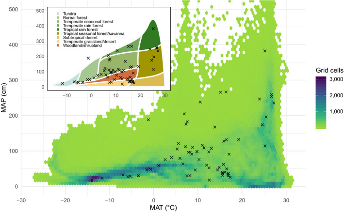
Distribution of COSORE datasets (black markers) in global climate space (WorldClim 2, Fick & Hijmans, 2017) of mean annual temperature (MAT) versus mean annual precipitation (MAP). Background colours indicate the number of half‐degree grid cells with each particular MAT–MAP combination. Inset plot shows the same points in Whittaker biome space (Ricklefs, 2008)

Flux observations, by IGBP (defined in Table 1), over time. Each square represents 5,000 observations, with categories of <5,000 observations rounded up so that they occupy a single square

Temporal density of COSORE datasets, by latitude of the observational site

Number of observations by day of year, for northern and southern hemisphere and by gas (CO₂ or CH₄), in the current COSORE datasets; the database currently has no CH₄ data from the Southern hemisphere (bottom left)

Temporal resolution (time interval between successive measurements, minutes; note logarithmic scale of x‐axis) of COSORE data

Dataset CO₂ fluxes (mostly soil respiration, but as noted above also some heterotrophic respiration and net ecosystem exchange) are generally log‐normally distributed in most IGBP classifications (Figure 8). The distribution of CH₄ is more complex, with most data clustered around 0 nmol m⁻² s⁻¹ but featuring long distribution tails to many orders of magnitude larger fluxes for both net uptake and release (Figure 9), due to the complexity and variety of biochemical processes involved in methane production and oxidation (Riley et al., 2011).

Distribution of CO₂ fluxes in COSORE datasets, by IGBP classification (cf. Table 1). For visual clarity this figure excludes fluxes <−1 and >10 µmol m⁻² s⁻¹ (210,752 observations, 2.6% of the data). Number of datasets (sites) making up data is given in parentheses after IGBP abbreviations in each panel

Distribution of CH₄ fluxes in COSORE datasets, by IGBP classification (cf. Table 1). For visual clarity this figure excludes some extreme values (18,719 observations or 4.5% of the data). Number of datasets (sites) making up data is given in parentheses after IGBP abbreviations in each panel. Positive values are emissions to the atmosphere, and negative values uptake by the soil

The COSORE team welcomes data contributions of soil‐atmosphere GHG flux data. We prioritize continuously measured (i.e. from automated systems including non‐chamber approaches) soil respiration datasets, but the database structure also accommodates (discontinuous, i.e. manual) data, as well as measurements of methane, net ecosystem exchange and heterotrophic respiration fluxes. Contributors receive a QA/QC report for all submissions, including details on invalid data, removed data, etc., and can then request corrections or changes before the data are uploaded and go ‘live’; contributors may also request a temporary embargo on their data. There currently is no standardized data template that contributors must follow, but we anticipate this changing before version 1.0 (planned for late 2020). There is no minimum data coverage required, either in time or space, although we suggest datasets should at a minimum span a growing season.

It is important to note that COSORE itself is not (yet) a permanent data repository: it is an open community database, but not institutionally backed in the manner of Figshare (https://figshare.com), DataONE (https://www.dataone.org), ESS‐DIVE (https://ess‐dive.lbl.gov/) or ORNL‐DAAC (https://daac.ornl.gov). Its design reflects extensive consultation with many of these groups for seamless interoperability and perhaps future merging. Nonetheless, currently we recommend that contributors deposit data in such a repository first, and provide its Digital Object Identifier (DOI) in the COSORE dataset metadata.

We use the GitHub issue tracker (https://github.com/bpbond/cosore/issues) to track and categorize user improvement suggestions, problems or errors with the R package code or database data, requests for new variables or functionality and/or asking questions on any other aspect of COSORE. The COSORE team welcomes questions, contributions and suggestions (see the ‘CODE_OF_CONDUCT.md’ file in the repository).

5. CONCLUSIONS: STRENGTHS, LIMITATIONS AND FUTURE DIRECTIONS

COSORE is a ‘coalition of the willing’ (sensu Novick et al., 2018), and intended to be a community‐driven resource for analyses of soil‐atmosphere GHG exchange. Possible analyses and next steps include syntheses, model evaluation and methodological developments, e.g. in gap filling algorithms (Gomez‐Casanovas et al., 2013; Zhao et al., 2020). Soil‐atmosphere GHG flux measurements can be used at individual sites to check and constrain estimates of other carbon cycle fluxes (Miao et al., 2017; e.g. Phillips et al., 2017). Aggregated data across multiple ecosystems can be used to test proposed conceptual frameworks and model structures for expanding our understanding beyond first‐order temperature driven responses, and improving representation of R _S and other GHG fluxes in global ecosystem models (Abramoff et al., 2017; Mitra et al., 2019; Subke & Bahn, 2010). Finally, open data and open‐source harmonization tools (with which to compile disparate datasets) support scientific reproducibility, serve as an educational resource (Mouromtsev & d’Aquin, 2016) and reduce loss of data over time (Powers & Hampton, 2018).

A crucial attribute of COSORE is its relationship to preexisting databases and efforts. The older Global Soil Respiration Database (SRDB, Bond‐Lamberty & Thomson, 2010) focuses on seasonal to annual fluxes, with monthly‐ and daily‐resolution offshoots of the SRDB (Jian, Steele, Day, et al., 2018; Jian, Steele, Thomas, et al., 2018) following similar designs. Others, such as ForC (Anderson‐Teixeira et al., 2018), take a broader scope and also focus on annual fluxes. We hope that the large volume of standardized, high‐frequency GHG flux data in COSORE will enable novel global scale syntheses, modelling activities, new insights driven by machine learning (Albert et al., 2017; Vargas et al., 2018) and conceptual advances (e.g. Petrakis et al., 2017) that are currently impossible. Linking COSORE data with other high‐resolution, open databases such as FLUXNET (Baldocchi et al., 2001) and the ICOS RI Carbon Portal (https://www.icos‐cp.eu/data‐services) is also likely to yield new insights.

COSORE has a number of limitations, some peculiar to the effort and others intrinsic to the discipline and community. First, as with many observations in the ecological and Earth sciences, it is spatially non‐representative at the global scale (Xu & Shang, 2016), and currently dominated by datasets from North America and East Asia (Figure 2). There are no datasets from Africa (cf. Epule, 2015) and little South American data. The IGBP representation is skewed as well (Figure 4), although the database's climate space coverage is reasonable (Figures 3 and 6). This spatial patchiness—a function of many factors including economic development, infrastructure, scientific investment—imposes significant restrictions on our ability to draw global inferences and analyses from extant observational data.

A second category of limitations arises from COSORE’s particular design. The database is oriented towards lightweight and minimal requirements, aiming for breadth over depth. This has benefits and costs. Having low barriers to entry shifts the burden of contributing data away from data providers, and keeping the design lightweight (with limited controlled vocabularies, ancillary data, etc.) has kept the burden on COSORE’s designers and maintainers manageable; we are acutely aware that every additional field or piece of information imposes a cost, both immediately (for implementation) and in perpetuity (for maintenance). This was the rationale behind focusing initially on previously uncollated continuous measurements: to maximize scientific impact in terms of labour involved. In fact, nothing in COSORE’s design itself precludes incorporation of spatially distributed, survey‐style measurements. COSORE also remains relatively immature, with e.g. no ‘level 2’ data product incorporating external data (e.g. Fick & Hijmans, 2017). This imposes an additional cost—of time and effort—on database users to locate and integrate externally available data themselves.

Finally, analyses using COSORE will be limited by the nature of soil respiration and other soil‐atmosphere gas flux measurements, and the state of the disciplines’ networks and community. Automated measurements trade space for time: the systems are more expensive and require dedicated power, and do not perform well under certain conditions, limiting their spatial and temporal coverage at many scales (Barba et al., 2018). There remains no institutionally backed network akin to AmeriFlux or ICOS, and while there have been efforts to integrate chamber flux data into these networks’ data products, this has inevitable consequences for continuity and consistency. There is also no standardization of measurement depths for ancillary measurements (e.g. soil temperature and moisture) in the manner of a top‐down network such as NEON (Schimel et al., 2007) or ICOS RI (Op de Beeck et al., 2018).

5.1. Future directions

As noted above, every expansion or addition to a database imposes both immediate development costs and unending maintenance costs. Nonetheless, there are some areas into which COSORE could be expanded. Many automated systems record isotopes and H₂O in addition to CO₂ and/or CH₄, and these data could be incorporated at relatively low cost; N₂O and NH₃ are other frequently measured GHGs. As noted above, downstream users would also benefit in the future from COSORE data premerged with global climate, ecological, field inventory or remote sensing data products. This feature is provided by the International Soil Radiocarbon Database (Lawrence et al., 2020), for example.

Currently, the COSORE team accepts flux data in any tabular format and performs unit conversion, restructuring and/or reformatting, etc., as needed. This was useful in the database's initial stages, as minimizing the work for contributors meant increased submissions. We intend however to shift this responsibility to data contributors before version 1.0, providing a template form that contributors must follow. This will allow for semiautomated data ingestion and follows the practices of many other earth sciences databases. Unusual or outlier measurements could also be automatically flagged for downstream users. More ambitiously, we have put substantial design work into ensuring interoperability so that COSORE data should flow relatively seamlessly into (or from) ESS‐DIVE, Ameriflux and ICOS RI. A long‐term vision is that COSORE data could, for example, automatically be made available in the larger community database. It is crucial, we believe, that COSORE contributors have assurances that their data contributions are traceable across versions and that it is not necessary to prepare and submit their data to multiple repositories. Finally, currently all data are included in the COSORE R package download. While convenient for users, this model will likely break down when the database doubles or triples in data volume. At that point, the data will need to be hosted elsewhere and downloaded only on demand.

Supporting information

Tables_S1‐S3

Click here for additional data file.^{(18.3KB, docx)}

ACKNOWLEDGEMENTS

The authors declare no conflicts of interest. This research was supported by the US Department of Energy (DOE), Office of Science, Biological and Environmental Research (BER) as part of the Terrestrial Ecosystem Sciences Program. D.S.C. was supported by the AmeriFlux Management Project funded by the DOE's Office of Science under Contract No. DE‐AC02‐05CH11231. S.C.P. was supported by ESS‐DIVE Community Funds Program, from the Data Management program within the Climate and Environmental Science Division of DOE BER. N.B. was supported by Swiss National Science Foundation project ICOS‐CH (20FI20_173691). J.Z. was supported by a joint Ph.D. program grant (201206300050) from the China Scholarship Council (CSC) and University College Dublin (UCD), Special Project on Hi‐Tech Innovation Capacity (KJCX20200301) and the Excellent Youth Scholars program from Beijing Academy of Agriculture and Forestry Sciences. B.O. was supported by the Higher Education Authority Programme for Research at Third Level Institutions Cycle 5 (PRTLI 5). E.A.D. was supported by DOE's Award DE‐SC0006741 and USDA grant 2014‐67003‐22073. W.L.S. was supported by grants from the US DOE (TES‐DE‐FOA‐0000749) and NSF (DEB‐1457805). D.S. and M.A.M. were supported by an Early Career Award through the DOE BER. J.W., Z.P. and H.K. were supported by a Special Project on Hi‐Tech Innovation Capacity grant (KJCX20200301) from the Beijing Academy of Agriculture and Forestry Sciences. S.‐C.C. was supported by the Ministry of Science and Technology, Taiwan. A.A.R., E.P., M.J.T., C.A.M. and J.E.D. were supported by Australian Research Council grants DP170102766, DP110105102 and DP160102452. C.L.P. and J.G. were supported by DOE #DE‐FG02‐05ER64048. C.L.P. is supported by the USDA Agricultural Research Service (project 2072‐12620‐001). The USDA is an equal opportunity provider and employer. J.W.R. was funded by NSF DEB‐0236502 and DEB‐0703561. M.P. was supported by the Swedish Infrastructure for Ecosystem Science. M.U. was supported by the Arctic Challenge for Sustainability II (JPMXD1420318865) project and JSPS KAKENHI Grant Numbers 23681004 and 26701002. J.J.A. and J.F.P.‐Q. were supported by the National Commission for Scientific and Technological Research (Chile) through grants FONDECYT 1171239, FONDEQUIP AIC‐37 and the Associative Research Program AFB170008. Q.Z. was supported by NSFC–NSF collaboration funding (P. R. China–U.S. 51861125102). A.R.D. acknowledges support from NSF #DBI‐1457897 and DOE Ameriflux Network Management Project core site funding to ChEAS core site cluster. R.L.S. acknowledges the USDA and DOE Office of Science for AmeriFlux core site support. The Pacific Northwest National Laboratory is operated for DOE by Battelle Memorial Institute under contract DE‐AC05‐76RL01830. ORNL is managed by the University of Tennessee‐Battelle, LLC, under contract DE‐AC05‐00OR22725 with DOE.

Bond‐Lamberty B, Christianson DS, Malhotra A, et al. COSORE: A community database for continuous soil respiration and other soil‐atmosphere greenhouse gas flux data. Glob Change Biol. 2020;26:7268–7283. 10.1111/gcb.15353

Notice: This manuscript has been authored by UT‐Battelle, LLC, under contract DE‐AC05‐00OR22725 with the US Department of Energy (DOE). The US government retains and the publisher, by accepting the article for publication, acknowledges that the US government retains a non‐exclusive, paid‐up, irrevocable, worldwide license to publish or reproduce the published form of this manuscript, or allow others to do so, for US government purposes. DOE will provide public access to these results of federally sponsored research in accordance with the DOE Public Access Plan (http://energy.gov/downloads/doe‐public‐access‐plan).

DATA AVAILABILITY STATEMENT

The data and code that support the findings of this study are openly available on GitHub at https://github.com/bpbond/cosore.

REFERENCES

Abramoff, R. Z. , Davidson, E. A. , & Finzi, A. C. (2017). A parsimonious modular approach to building a mechanistic belowground carbon and nitrogen model. Journal of Geophysical Research: Biogeosciences, 122(9), 2418–2434. 10.1002/2017JG003796 [DOI] [Google Scholar]
Albert, L. P. , Keenan, T. F. , Burns, S. P. , Huxman, T. E. , & Monson, R. K. (2017). Climate controls over ecosystem metabolism: Insights from a fifteen‐year inductive artificial neural network synthesis for a subalpine forest. Oecologia, 184(1), 25–41. 10.1007/s00442-017-3853-0 [DOI] [PubMed] [Google Scholar]
Anderson‐Teixeira, K. J. , Wang, M. M. H. , McGarvey, J. C. , Herrmann, V. , Tepley, A. J. , Bond‐Lamberty, B. , & LeBauer, D. S. (2018). ForC: A global database of forest carbon stocks and fluxes. Ecology, 99(6), 1507 10.1002/ecy.2229 [DOI] [PubMed] [Google Scholar]
Baldocchi, D. , Falge, E. , Gu, L. , Olson, R. , Hollinger, D. , Running, S. , Anthoni, P. , Bernhofer, C. H. , Davis, K. , Evans, R. , Fuentes, J. , Goldstein, A. , Katul, G. , Law, B. , Lee, X. , Malhi, Y. , Meyers, T. , Munger, W. , Oechel, W. , … Wofsy, S. (2001). FLUXNET: A new tool to study the temporal and spatial variability of ecosystem‐scale carbon dioxide, water vapor, and energy flux densities. Bulletin of the American Meteorological Society, 82(11), 2415–2434. 10.1175/1520-0477(2001)082<2415:FANTTS>2.3.CO;2 [DOI] [Google Scholar]
Barba, J. , Cueva, A. , Bahn, M. , Barron‐Gafford, G. A. , Bond‐Lamberty, B. , Hanson, P. J. , Jaimes, A. , Kulmala, L. , Pumpanen, J. , Scott, R. L. , Wohlfahrt, G. , & Vargas, R. (2018). Comparing ecosystem and soil respiration: Review and key challenges of tower‐based and soil measurements. Agricultural and Forest Meteorology, 249(Suppl. C), 434–443. 10.1016/j.agrformet.2017.10.028 [DOI] [Google Scholar]
Bond‐Lamberty, B. (2018). New techniques and data for understanding the global soil respiration flux. Earth’s Future, 6(9), 1176–1180. 10.1029/2018EF000866 [DOI] [Google Scholar]
Bond‐Lamberty, B. , & Thomson, A. (2010). A global database of soil respiration data. Biogeosciences, 7, 1915–1926. 10.5194/bg-7-1915-2010 [DOI] [Google Scholar]
Brannon, E. Q. , Moseman‐Valtierra, S. M. , Rella, C. W. , Martin, R. M. , Chen, X. , & Tang, J. (2016). Evaluation of laser‐based spectrometers for greenhouse gas flux measurements in coastal marshes. Limnology and Oceanography, Methods, 14(7), 466–476. 10.1002/lom3.10105 [DOI] [Google Scholar]
Courtois, E. A. , Stahl, C. , Burban, B. , Van den Berge, J. , Berveiller, D. , Bréchet, L. , Soong, J. L. , Arriga, N. , Peñuelas, J. , & Janssens, I. A. (2019). Automatic high‐frequency measurements of full soil greenhouse gas fluxes in a tropical forest. Biogeosciences, 16(3), 785–796. 10.5194/bg-16-785-2019 [DOI] [Google Scholar]
Davidson, E. A. , Savage, K. E. , Bolstad, P. V. , Clark, D. A. , Curtis, P. S. , Ellsworth, D. S. , Hanson, P. J. , Law, B. E. , Luo, Y. , Pregitzer, K. S. , Randolph, J. C. , & Zak, D. R. (2002). Belowground carbon allocation in forests estimated from litterfall and IRGA‐based soil respiration measurements. Agricultural and Forest Meteorology, 113, 39–51. 10.1016/S0168-1923(02)00101-6 [DOI] [Google Scholar]
Detto, M. , Verfaillie, J. , Anderson, F. , Xu, L. , & Baldocchi, D. (2011). Comparing laser‐based open‐ and closed‐path gas analyzers to measure methane fluxes using the eddy covariance method. Agricultural and Forest Meteorology, 151(10), 1312–1324. 10.1016/j.agrformet.2011.05.014 [DOI] [Google Scholar]
Diefenderfer, H. L. , Cullinan, V. I. , & Borde, A. B. (2018). High‐frequency greenhouse gas flux measurement system detects winter storm surge effects on salt marsh. Global Change Biology [online]. 10.1111/gcb.14430 [DOI] [PubMed] [Google Scholar]
Drake, J. E. , Macdonald, C. A. , Tjoelker, M. G. , Reich, P. B. , Singh, B. K. , Anderson, I. C. , & Ellsworth, D. S. (2018). Three years of soil respiration in a mature eucalypt woodland exposed to atmospheric CO₂ enrichment. Biogeochemistry, 139(1), 85–101. 10.1007/s10533-018-0457-7 [DOI] [Google Scholar]
DuBois, A. B. , Fowler, R. C. , Soffer, A. , & Fenn, W. O. (1952). Alveolar CO₂ measured by expiration into the rapid infrared gas analyzer. Journal of Applied Physiology. 10.1152/jappl.1952.4.7.526 [DOI] [PubMed] [Google Scholar]
Epule, T. E. (2015). A new compendium of soil respiration data for Africa. Challenges, 6(1), 88–97. 10.3390/challe6010088 [DOI] [Google Scholar]
Fick, S. E. , & Hijmans, R. J. (2017). WorldClim 2: New 1‐km spatial resolution climate surfaces for global land areas. International Journal of Climatology. 10.1002/joc.5086 [DOI] [Google Scholar]
Friedlingstein, P. , Jones, M. W. , O'Sullivan, M. , Andrew, R. M. , Hauck, J. , Peters, G. P. , Peters, W. , Pongratz, J. , Sitch, S. , Le Quéré, C. , Bakker, D. C. E. , Canadell, J. G. , Ciais, P. , Jackson, R. B. , Anthoni, P. , Barbero, L. , Bastos, A. , Bastrikov, V. , Becker, M. , … Zaehle, S. (2019). Global carbon budget 2019. Earth System Science Data, 11(4), 1783–1838. 10.5194/essd-11-1783-2019 [DOI] [Google Scholar]
Gomez‐Casanovas, N. , Anderson‐Teixeira, K. , Zeri, M. , Bernacchi, C. J. , & DeLucia, E. H. (2013). Gap filling strategies and error in estimating annual soil respiration. Global Change Biology, 19(6), 1941–1952. 10.1111/gcb.12127 [DOI] [PubMed] [Google Scholar]
Goulden, M. L. , & Crill, P. M. (1997). Automated measurements of CO₂ exchange at the moss surface of a black spruce forest. Tree Physiology, 17, 537–542. [DOI] [PubMed] [Google Scholar]
Gruber, N. , & Galloway, J. N. (2008). An Earth‐system perspective of the global nitrogen cycle. Nature, 451(7176), 293–296. 10.1038/nature06592 [DOI] [PubMed] [Google Scholar]
Hirano, T. , Kim, H. , & Tanaka, Y. (2003). Long‐term half‐hourly measurement of soil CO₂ concentration and soil respiration in a temperate deciduous forest. Journal of Geophysical Research, D: Atmospheres, 108(D20). 10.1029/2003JD003766 [DOI] [Google Scholar]
Högberg, P. , Nordgren, A. , Buchmann, N. , Taylor, A. F. S. , Ekblad, A. , Högberg, M. N. , Nyberg, G. , Ottosson‐Löfvenius, M. , & Read, D. J. (2001). Large‐scale forest girdling shows that current photosynthesis drives soil respiration. Nature, 411(6839), 789–792. [DOI] [PubMed] [Google Scholar]
Irvine, J. , & Law, B. E. (2002). Contrasting soil respiration in young and old‐growth ponderosa pine forests. Global Change Biology, 8, 1183–1194. 10.1046/j.1365-2486.2002.00544.x [DOI] [Google Scholar]
Järveoja, J. , Nilsson, M. B. , Gažovič, M. , Crill, P. M. , & Peichl, M. (2018). Partitioning of the net CO₂ exchange using an automated chamber system reveals plant phenology as key control of production and respiration fluxes in a boreal peatland. Global Change Biology, 24(8), 3436–3451. 10.1111/gcb.14292 [DOI] [PubMed] [Google Scholar]
Jassal, R. S. , Black, T. A. , Novak, M. D. , Morgenstern, K. , Nesic, Z. , & Gaumont‐Guay, D. (2005). Relationship between soil CO₂ concentrations and forest‐floor CO₂ effluxes. Agricultural and Forest Meteorology, 130(3–4), 176–192. 10.1016/j.agrformet.2005.03.005 [DOI] [Google Scholar]
Jian, J. , Steele, M. K. , Day, S. D. , Quinn Thomas, R. , & Hodges, S. C. (2018). Measurement strategies to account for soil respiration temporal heterogeneity across diverse regions. Soil Biology and Biochemistry, 125, 167–177. 10.1016/j.soilbio.2018.07.003 [DOI] [Google Scholar]
Jian, J. , Steele, M. K. , Thomas, R. Q. , Day, S. D. , & Hodges, S. C. (2018). Constraining estimates of global soil respiration by quantifying sources of variability. Global Change Biology, 24(9), 4143–4159. 10.1111/gcb.14301 [DOI] [PubMed] [Google Scholar]
Kahle, D. , & Wickham, H. (2013). ggmap: Spatial visualization with ggplot2. The R Journal, 5(1), 144–161. https://journal.r‐project.org/archive/2013‐1/kahle‐wickham.pdf [Google Scholar]
Kirschke, S. , Bousquet, P. , Ciais, P. , Saunois, M. , Canadell, J. G. , Dlugokencky, E. J. , Bergamaschi, P. , Bergmann, D. , Blake, D. R. , Bruhwiler, L. , Cameron‐Smith, P. , Castaldi, S. , Chevallier, F. , Feng, L. , Fraser, A. , Heimann, M. , Hodson, E. L. , Houweling, S. , Josse, B. , … Zeng, G. (2013). Three decades of global methane sources and sinks. Nature Geoscience, 6(10), 813–823. 10.1038/ngeo1955 [DOI] [Google Scholar]
Knox, S. H. , Jackson, R. B. , Poulter, B. , McNicol, G. , Fluet‐Chouinard, E. , Zhang, Z. , Hugelius, G. , Bousquet, P. , Canadell, J. G. , Saunois, M. , Papale, D. , Chu, H. , Keenan, T. F. , Baldocchi, D. , Torn, M. S. , Mammarella, I. , Trotta, C. , Aurela, M. , Bohrer, G. , … Zona, D. (2019). FLUXNET‐CH4 synthesis activity: Objectives, observations, and future directions. Bulletin of the American Meteorological Society, 100(12), 2607–2632. 10.1175/BAMS-D-18-0268.1 [DOI] [Google Scholar]
Latimer, R. N. C. , & Risk, D. A. (2016). An inversion approach for determining distribution of production and temperature sensitivity of soil respiration. Biogeosciences, 13(7), 2111–2122. 10.5194/bg-13-2111-2016 [DOI] [Google Scholar]
Lavoie, M. , Owens, J. , & Risk, D. (2012). A new method for real‐time monitoring of soil CO₂ efflux. Methods in Ecology and Evolution / British Ecological Society, 3(5), 889–897. 10.1111/j.2041-210X.2012.00214.x [DOI] [Google Scholar]
Lavoie, M. , Phillips, C. L. , & Risk, D. (2015). A practical approach for uncertainty quantification of high‐frequency soil respiration using Forced Diffusion chambers. Journal of Geophysical Research: Biogeosciences, 120(1), 128–146. 10.1002/2014JG002773 [DOI] [Google Scholar]
Lawrence, C. R. , Beem‐Miller, J. , Hoyt, A. M. , Monroe, G. , Sierra, C. A. , Stoner, S. , Heckman, K. , Blankinship, J. C. , Crow, S. E. , McNicol, G. , Trumbore, S. , Levine, P. A. , Vindušková, O. , Todd‐Brown, K. , Rasmussen, C. , Hicks Pries, C. E. , Schädel, C. , McFarlane, K. , Doetterl, S. , … Wagai, R. (2020). An open‐source database for the synthesis of soil radiocarbon data: International Soil Radiocarbon Database (ISRaD) version 1.0. Earth System Science Data, 12(1), 61–76. 10.5194/essd-12-61-2020 [DOI] [Google Scholar]
Loveland, T. R. , Reed, B. C. , Brown, J. F. , Ohlen, D. O. , Zhu, Z. , Yang, L. , & Merchant, J. W. (2000). Development of a global land cover characteristics database and IGBP DISCover from 1 km AVHRR data. International Journal of Remote Sensing, 21(6–7), 1303–1330. 10.1080/014311600210191 [DOI] [Google Scholar]
Lowndes, J. S. S. , Best, B. D. , Scarborough, C. , Afflerbach, J. C. , Frazier, M. R. , O’Hara, C. C. , Jiang, N. , & Halpern, B. S. (2017). Our path to better science in less time using open data science tools. Nature Ecology & Evolution, 1(6), 160 10.1038/s41559-017-0160 [DOI] [PubMed] [Google Scholar]
Miao, G. , Noormets, A. , Domec, J.‐C. , Fuentes, M. , Trettin, C. C. , Sun, G. , McNulty, S. G. , & King, J. S. (2017). Hydrology and microtopography control carbon dynamics in wetlands: Implications in partitioning ecosystem respiration in a coastal plain forested wetland. Agricultural and Forest Meteorology, 247, 343–355. 10.1016/j.agrformet.2017.08.022 [DOI] [Google Scholar]
Migliavacca, M. , Reichstein, M. , Richardson, A. D. , Mahecha, M. D. , Cremonese, E. , Delpierre, N. , Galvagno, M. , Law, B. E. , Wohlfahrt, G. , Black, T. A. , Carvalhais, N. , Ceccherini, G. , Chen, J. , Gobron, N. , Koffi, E. , Munger, J. W. , Perez‐Priego, O. , Robustelli, M. , Tomelleri, E. , & Cescatti, A. (2015). Influence of physiological phenology on the seasonal pattern of ecosystem respiration in deciduous forests. Global Change Biology, 21(1), 363–376. 10.1111/gcb.12671 [DOI] [PubMed] [Google Scholar]
Mitra, B. , Miao, G. , Minick, K. , McNulty, S. G. , Sun, G. , Gavazzi, M. , King, J. S. , & Noormets, A. (2019). Disentangling the effects of temperature, moisture, and substrate availability on soil CO₂ efflux. Journal of Geophysical Research: Biogeosciences, 124(7), 2060–2075. 10.1029/2019JG005148 [DOI] [Google Scholar]
Mouromtsev, D. , & d’Aquin, M. (2016). Open data for education: Linked, shared, and reusable data for teaching and learning. Springer; https://play.google.com/store/books/details?id=AwvNCwAAQBAJ [Google Scholar]
Nay, S. M. , Mattson, K. G. , & Bormann, B. T. (1994). Biases of chamber methods for measuring Soil CO₂ efflux demonstrated with a laboratory apparatus. Ecology, 75(8), 2460 10.2307/1940900 [DOI] [Google Scholar]
Neubauer, S. C. , & Megonigal, J. P. (2015). Moving beyond global warming potentials to quantify the climatic role of ecosystems. Ecosystems, 18(6), 1000–1013. 10.1007/s10021-015-9879-4 [DOI] [Google Scholar]
Novick, K. A. , Biederman, J. A. , Desai, A. R. , Litvak, M. E. , Moore, D. J. P. , Scott, R. L. , & Torn, M. S. (2018). The AmeriFlux network: A coalition of the willing. Agricultural and Forest Meteorology, 249(Suppl. C), 444–456. 10.1016/j.agrformet.2017.10.009 [DOI] [Google Scholar]
Op de Beeck, M. , Gielen, B. , Merbold, L. , Ayres, E. , Serrano‐Ortiz, P. , Acosta, M. , Pavelka, M. , Montagnani, L. , Nilsson, M. , Klemedtsson, L. , Vincke, C. , De Ligne, A. , Moureaux, C. , Marañon‐Jimenez, S. , Saunders, M. , Mereu, S. , & Hörtnagl, L. (2018). Soil‐meteorological measurements at ICOS monitoring stations in terrestrial ecosystems. International Agrophysics, 32(4), 619–631. 10.1515/intag-2017-0041 [DOI] [Google Scholar]
Petrakis, S. , Barba, J. , Bond‐Lamberty, B. , & Vargas, R. (2017). Using greenhouse gas fluxes to define soil functional types. Plant and Soil, 1–10, 10.1007/s11104-017-3506-4 [DOI] [Google Scholar]
Petrakis, S. , Seyfferth, A. , Kan, J. , Inamdar, S. , & Vargas, R. (2017). Influence of experimental extreme water pulses on greenhouse gas emissions from soils. Biogeochemistry, 133(2), 147–164. 10.1007/s10533-017-0320-2 [DOI] [Google Scholar]
Phillips, C. L. , Bond‐Lamberty, B. , Desai, A. R. , Lavoie, M. , Risk, D. , Tang, J. , Todd‐Brown, K. , & Vargas, R. (2017). The value of soil respiration measurements for interpreting and modeling terrestrial carbon cycling. Plant and Soil, 413(1–2), 1–25. 10.1007/s11104-016-3084-x [DOI] [Google Scholar]
Powers, S. M. , & Hampton, S. E. (2018). Open science, reproducibility, and transparency in ecology. Ecological Applications, 29(1). 10.1002/eap.1822 [DOI] [PubMed] [Google Scholar]
Pumpanen, J. , Kolari, P. , Ilvesniemi, H. , Minkkinen, K. , Vesala, T. , Niinistö, S. , Lohila, A. , Larmola, T. , Morero, M. , Pihlatie, M. , Janssens, I. A. , Curiel Yuste, J. , Grünzweig, J. M. , Reth, S. , Subke, J.‐A. , Savage, K. E. , Kutsch, W. L. , Østreng, G. , Ziegler, W. , … Hari, P. (2004). Comparison of different chamber techniques for measuring soil CO₂ flux. Agricultural and Forest Meteorology, 123(3–4), 159–176. 10.1016/j.agrformet.2003.12.001 [DOI] [Google Scholar]
R Core Team . (2019). R: A language and environment for statistical computing, version 3.6.1. R Foundation for Statistical Computing; https://www.R‐project.org/ [Google Scholar]
Raich, J. W. (2017). Temporal variability of soil respiration in experimental tree plantations in lowland Costa Rica. Forests, Trees and Livelihoods, 8(2), 40 10.3390/f8020040 [DOI] [Google Scholar]
Raich, J. W. , & Potter, C. S. (1995). Global patterns of carbon dioxide emissions from soils. Global Biochemical Cycles, 9(1), 23–36. [Google Scholar]
Rayment, M. B. , & Jarvis, P. G. (1997). An improved open chamber system for measuring soil CO₂ effluxes in the field. Journal of Geophysical Research, D: Atmospheres, 102(D24), 28779–28784. 10.1029/97JD01103 [DOI] [Google Scholar]
Ricklefs, R. E. (2008). The economy of nature. W.H. Freeman; 620 pp. [Google Scholar]
Riley, W. J. , Subin, Z. M. , Lawrence, D. M. , Swenson, S. C. , Torn, M. S. , Meng, L. , Mahowald, N. M. , & Hess, P. (2011). Barriers to predicting changes in global terrestrial methane fluxes: analyses using CLM4Me, a methane biogeochemistry model integrated in CESM. Biogeosciences, 8, 1925–1953. 10.5194/bg-8-1925-2011 [DOI] [Google Scholar]
Saunois, M. , Bousquet, P. , Poulter, B. , Peregon, A. , Ciais, P. , Canadell, J. G. , Dlugokencky, E. J. , Etiope, G. , Bastviken, D. , Houweling, S. , Janssens‐Maenhout, G. , Tubiello, F. N. , Castaldi, S. , Jackson, R. B. , Alexe, M. , Arora, V. K. , Beerling, D. J. , Bergamaschi, P. , Blake, D. R. , … Zhu, Q. (2016). The global methane budget 2000–2012. Earth System Science Data, 8(2), 697–751. 10.5194/essd-8-697-2016 [DOI] [Google Scholar]
Savage, K. , Phillips, R. , & Davidson, E. (2014). High temporal frequency measurements of greenhouse gas emissions from soils. Biogeosciences, 11(10), 2709–2720. 10.5194/bg-11-2709-2014 [DOI] [Google Scholar]
Schädel, C. , Beem‐Miller, J. , Aziz Rad, M. , Crow, S. E. , Hicks Pries, C. E. , Ernakovich, J. , Hoyt, A. M. , Plante, A. , Stoner, S. , Treat, C. C. , & Sierra, C. A. (2020). Decomposability of soil organic matter over time: the Soil Incubation Database (SIDb, version 1.0) and guidance for incubation procedures. Earth System Science Data, 12(3), 1511–1524. 10.5194/essd-12-1511-2020 [DOI] [Google Scholar]
Schimel, D. , Hargrove, W. , Hoffman, F. , & MacMahon, J. (2007). NEON: A hierarchically designed national ecological network. Frontiers in Ecology and the Environment, 5(2), 59 10.1890/1540-9295(2007)5[59:NAHDNE]2.0.CO;2 [DOI] [Google Scholar]
Subke, J.‐A. , & Bahn, M. (2010). On the “temperature sensitivity” of soil respiration: Can we use the immeasurable to predict the unknown? Soil Biology & Biochemistry, 42(9), 1653–1656. 10.1016/j.soilbio.2010.05.026 [DOI] [PMC free article] [PubMed] [Google Scholar]
Subke, J.‐A. , Inglima, I. , & Cotrufo, M. F. (2006). Trends and methodological impacts in soil CO₂ efflux partitioning: A metaanalytical review. Global Change Biology, 12(2), 921–943. 10.1111/j.1365-2486.2006.01117.x [DOI] [Google Scholar]
Tang, G. , Zheng, J. , Xu, X. , Yang, Z. , Graham, D. E. , Gu, B. , Painter, S. L. , & Thornton, P. E. (2016). Biogeochemical modeling of CO₂ and CH₄ production in anoxic Arctic soil microcosms. Biogeosciences, 13(17), 5021–5041. 10.5194/bg-13-5021-2016 [DOI] [Google Scholar]
Tang, J. , Baldocchi, D. D. , Qi, Y. , & Xu, L. (2003). Assessing soil CO₂ efflux using continuous measurements of CO₂ profiles in soils with small solid‐state sensors. Agricultural and Forest Meteorology, 118, 207–220. 10.1016/S0168-1923(03)00112-6 [DOI] [Google Scholar]
Tian, H. , Chen, G. , Lu, C. , Xu, X. , Ren, W. , Zhang, B. , Banger, K. , Tao, B. , Pan, S. , Liu, M. , Zhang, C. , Bruhwiler, L. , & Wofsy, S. (2015). Global methane and nitrous oxide emissions from terrestrial ecosystems due to multiple environmental changes. Ecosystem Health and Sustainability, 1(1), 1–20. 10.1890/EHS14-0015.1 [DOI] [Google Scholar]
Vargas, R. , Sánchez‐Cañete P., E. , Serrano‐Ortiz, P. , Curiel Yuste, J. , Domingo, F. , López‐Ballesteros, A. , & Oyonarte, C. (2018). Hot‐moments of soil CO₂ efflux in a water‐limited grassland. Soil Systems, 2(3), 47 10.3390/soilsystems2030047 [DOI] [Google Scholar]
Volkmann, T. H. M. , Haberer, K. , Gessler, A. , & Weiler, M. (2016). High‐resolution isotope measurements resolve rapid ecohydrological dynamics at the soil–plant interface. The New Phytologist, 210(3), 839–849. 10.1111/nph.13868 [DOI] [PubMed] [Google Scholar]
Wang, X. , Wang, C. , & Bond‐Lamberty, B. (2017). Quantifying and reducing the differences in forest CO₂‐fluxes estimated by eddy covariance, biometric and chamber methods: A global synthesis. Agricultural and Forest Meteorology, 247, 93–103. 10.1016/j.agrformet.2017.07.023 [DOI] [Google Scholar]
Wolkovich, E. M. , Regetz, J. , & O’Connor, M. I. (2012). Advances in global change research require open science by individual researchers. Global Change Biology, 18(7), 2102–2110. 10.1111/j.1365-2486.2012.02693.x [DOI] [Google Scholar]
Xu, L. , Furtaw, M. D. , Madsen, R. A. , Garcia, R. L. , Anderson, D. J. , & McDermitt, D. K. (2006). On maintaining pressure equilibrium between a soil CO₂ flux chamber and the ambient air. Journal of Geophysical Research, 111(D8), 225 10.1029/2005JD006435 [DOI] [Google Scholar]
Xu, M. , & Shang, H. (2016). Contribution of soil respiration to the global carbon equation. Journal of Plant Physiology, 203, 16–28. 10.1016/j.jplph.2016.08.007 [DOI] [PubMed] [Google Scholar]
Zhao, J. (2003). Data‐flow‐based unit testing of aspect‐oriented programs. Proceedings 27th Annual International Computer Software and Applications Conference COMPAC, 2003, 188–197. 10.1109/CMPSAC.2003.1245340 [DOI] [Google Scholar]
Zhao, J. , Lange, H. , & Meissner, H. (2020). Gap‐filling continuously‐measured soil respiration data: A highlight of time‐series‐based methods. Agricultural and Forest Meteorology, 285–286, 107912 10.1016/j.agrformet.2020.107912 [DOI] [Google Scholar]

Associated Data

This section collects any data citations, data availability statements, or supplementary materials included in this article.

Supplementary Materials

Tables_S1‐S3

Click here for additional data file.^{(18.3KB, docx)}

Data Availability Statement

The data and code that support the findings of this study are openly available on GitHub at https://github.com/bpbond/cosore.

[gcb15353-bib-0001] Abramoff, R. Z. , Davidson, E. A. , & Finzi, A. C. (2017). A parsimonious modular approach to building a mechanistic belowground carbon and nitrogen model. Journal of Geophysical Research: Biogeosciences, 122(9), 2418–2434. 10.1002/2017JG003796 [DOI] [Google Scholar]

[gcb15353-bib-0002] Albert, L. P. , Keenan, T. F. , Burns, S. P. , Huxman, T. E. , & Monson, R. K. (2017). Climate controls over ecosystem metabolism: Insights from a fifteen‐year inductive artificial neural network synthesis for a subalpine forest. Oecologia, 184(1), 25–41. 10.1007/s00442-017-3853-0 [DOI] [PubMed] [Google Scholar]

[gcb15353-bib-0003] Anderson‐Teixeira, K. J. , Wang, M. M. H. , McGarvey, J. C. , Herrmann, V. , Tepley, A. J. , Bond‐Lamberty, B. , & LeBauer, D. S. (2018). ForC: A global database of forest carbon stocks and fluxes. Ecology, 99(6), 1507 10.1002/ecy.2229 [DOI] [PubMed] [Google Scholar]

[gcb15353-bib-0004] Baldocchi, D. , Falge, E. , Gu, L. , Olson, R. , Hollinger, D. , Running, S. , Anthoni, P. , Bernhofer, C. H. , Davis, K. , Evans, R. , Fuentes, J. , Goldstein, A. , Katul, G. , Law, B. , Lee, X. , Malhi, Y. , Meyers, T. , Munger, W. , Oechel, W. , … Wofsy, S. (2001). FLUXNET: A new tool to study the temporal and spatial variability of ecosystem‐scale carbon dioxide, water vapor, and energy flux densities. Bulletin of the American Meteorological Society, 82(11), 2415–2434. 10.1175/1520-0477(2001)082<2415:FANTTS>2.3.CO;2 [DOI] [Google Scholar]

[gcb15353-bib-0005] Barba, J. , Cueva, A. , Bahn, M. , Barron‐Gafford, G. A. , Bond‐Lamberty, B. , Hanson, P. J. , Jaimes, A. , Kulmala, L. , Pumpanen, J. , Scott, R. L. , Wohlfahrt, G. , & Vargas, R. (2018). Comparing ecosystem and soil respiration: Review and key challenges of tower‐based and soil measurements. Agricultural and Forest Meteorology, 249(Suppl. C), 434–443. 10.1016/j.agrformet.2017.10.028 [DOI] [Google Scholar]

[gcb15353-bib-0006] Bond‐Lamberty, B. (2018). New techniques and data for understanding the global soil respiration flux. Earth’s Future, 6(9), 1176–1180. 10.1029/2018EF000866 [DOI] [Google Scholar]

[gcb15353-bib-0007] Bond‐Lamberty, B. , & Thomson, A. (2010). A global database of soil respiration data. Biogeosciences, 7, 1915–1926. 10.5194/bg-7-1915-2010 [DOI] [Google Scholar]

[gcb15353-bib-0008] Brannon, E. Q. , Moseman‐Valtierra, S. M. , Rella, C. W. , Martin, R. M. , Chen, X. , & Tang, J. (2016). Evaluation of laser‐based spectrometers for greenhouse gas flux measurements in coastal marshes. Limnology and Oceanography, Methods, 14(7), 466–476. 10.1002/lom3.10105 [DOI] [Google Scholar]

[gcb15353-bib-0009] Courtois, E. A. , Stahl, C. , Burban, B. , Van den Berge, J. , Berveiller, D. , Bréchet, L. , Soong, J. L. , Arriga, N. , Peñuelas, J. , & Janssens, I. A. (2019). Automatic high‐frequency measurements of full soil greenhouse gas fluxes in a tropical forest. Biogeosciences, 16(3), 785–796. 10.5194/bg-16-785-2019 [DOI] [Google Scholar]

[gcb15353-bib-0010] Davidson, E. A. , Savage, K. E. , Bolstad, P. V. , Clark, D. A. , Curtis, P. S. , Ellsworth, D. S. , Hanson, P. J. , Law, B. E. , Luo, Y. , Pregitzer, K. S. , Randolph, J. C. , & Zak, D. R. (2002). Belowground carbon allocation in forests estimated from litterfall and IRGA‐based soil respiration measurements. Agricultural and Forest Meteorology, 113, 39–51. 10.1016/S0168-1923(02)00101-6 [DOI] [Google Scholar]

[gcb15353-bib-0011] Detto, M. , Verfaillie, J. , Anderson, F. , Xu, L. , & Baldocchi, D. (2011). Comparing laser‐based open‐ and closed‐path gas analyzers to measure methane fluxes using the eddy covariance method. Agricultural and Forest Meteorology, 151(10), 1312–1324. 10.1016/j.agrformet.2011.05.014 [DOI] [Google Scholar]

[gcb15353-bib-0070] Diefenderfer, H. L. , Cullinan, V. I. , & Borde, A. B. (2018). High‐frequency greenhouse gas flux measurement system detects winter storm surge effects on salt marsh. Global Change Biology [online]. 10.1111/gcb.14430 [DOI] [PubMed] [Google Scholar]

[gcb15353-bib-0012] Drake, J. E. , Macdonald, C. A. , Tjoelker, M. G. , Reich, P. B. , Singh, B. K. , Anderson, I. C. , & Ellsworth, D. S. (2018). Three years of soil respiration in a mature eucalypt woodland exposed to atmospheric CO₂ enrichment. Biogeochemistry, 139(1), 85–101. 10.1007/s10533-018-0457-7 [DOI] [Google Scholar]

[gcb15353-bib-0013] DuBois, A. B. , Fowler, R. C. , Soffer, A. , & Fenn, W. O. (1952). Alveolar CO₂ measured by expiration into the rapid infrared gas analyzer. Journal of Applied Physiology. 10.1152/jappl.1952.4.7.526 [DOI] [PubMed] [Google Scholar]

[gcb15353-bib-0014] Epule, T. E. (2015). A new compendium of soil respiration data for Africa. Challenges, 6(1), 88–97. 10.3390/challe6010088 [DOI] [Google Scholar]

[gcb15353-bib-0015] Fick, S. E. , & Hijmans, R. J. (2017). WorldClim 2: New 1‐km spatial resolution climate surfaces for global land areas. International Journal of Climatology. 10.1002/joc.5086 [DOI] [Google Scholar]

[gcb15353-bib-0016] Friedlingstein, P. , Jones, M. W. , O'Sullivan, M. , Andrew, R. M. , Hauck, J. , Peters, G. P. , Peters, W. , Pongratz, J. , Sitch, S. , Le Quéré, C. , Bakker, D. C. E. , Canadell, J. G. , Ciais, P. , Jackson, R. B. , Anthoni, P. , Barbero, L. , Bastos, A. , Bastrikov, V. , Becker, M. , … Zaehle, S. (2019). Global carbon budget 2019. Earth System Science Data, 11(4), 1783–1838. 10.5194/essd-11-1783-2019 [DOI] [Google Scholar]

[gcb15353-bib-0017] Gomez‐Casanovas, N. , Anderson‐Teixeira, K. , Zeri, M. , Bernacchi, C. J. , & DeLucia, E. H. (2013). Gap filling strategies and error in estimating annual soil respiration. Global Change Biology, 19(6), 1941–1952. 10.1111/gcb.12127 [DOI] [PubMed] [Google Scholar]

[gcb15353-bib-0018] Goulden, M. L. , & Crill, P. M. (1997). Automated measurements of CO₂ exchange at the moss surface of a black spruce forest. Tree Physiology, 17, 537–542. [DOI] [PubMed] [Google Scholar]

[gcb15353-bib-0019] Gruber, N. , & Galloway, J. N. (2008). An Earth‐system perspective of the global nitrogen cycle. Nature, 451(7176), 293–296. 10.1038/nature06592 [DOI] [PubMed] [Google Scholar]

[gcb15353-bib-0020] Hirano, T. , Kim, H. , & Tanaka, Y. (2003). Long‐term half‐hourly measurement of soil CO₂ concentration and soil respiration in a temperate deciduous forest. Journal of Geophysical Research, D: Atmospheres, 108(D20). 10.1029/2003JD003766 [DOI] [Google Scholar]

[gcb15353-bib-0021] Högberg, P. , Nordgren, A. , Buchmann, N. , Taylor, A. F. S. , Ekblad, A. , Högberg, M. N. , Nyberg, G. , Ottosson‐Löfvenius, M. , & Read, D. J. (2001). Large‐scale forest girdling shows that current photosynthesis drives soil respiration. Nature, 411(6839), 789–792. [DOI] [PubMed] [Google Scholar]

[gcb15353-bib-0022] Irvine, J. , & Law, B. E. (2002). Contrasting soil respiration in young and old‐growth ponderosa pine forests. Global Change Biology, 8, 1183–1194. 10.1046/j.1365-2486.2002.00544.x [DOI] [Google Scholar]

[gcb15353-bib-0023] Järveoja, J. , Nilsson, M. B. , Gažovič, M. , Crill, P. M. , & Peichl, M. (2018). Partitioning of the net CO₂ exchange using an automated chamber system reveals plant phenology as key control of production and respiration fluxes in a boreal peatland. Global Change Biology, 24(8), 3436–3451. 10.1111/gcb.14292 [DOI] [PubMed] [Google Scholar]

[gcb15353-bib-0024] Jassal, R. S. , Black, T. A. , Novak, M. D. , Morgenstern, K. , Nesic, Z. , & Gaumont‐Guay, D. (2005). Relationship between soil CO₂ concentrations and forest‐floor CO₂ effluxes. Agricultural and Forest Meteorology, 130(3–4), 176–192. 10.1016/j.agrformet.2005.03.005 [DOI] [Google Scholar]

[gcb15353-bib-0025] Jian, J. , Steele, M. K. , Day, S. D. , Quinn Thomas, R. , & Hodges, S. C. (2018). Measurement strategies to account for soil respiration temporal heterogeneity across diverse regions. Soil Biology and Biochemistry, 125, 167–177. 10.1016/j.soilbio.2018.07.003 [DOI] [Google Scholar]

[gcb15353-bib-0026] Jian, J. , Steele, M. K. , Thomas, R. Q. , Day, S. D. , & Hodges, S. C. (2018). Constraining estimates of global soil respiration by quantifying sources of variability. Global Change Biology, 24(9), 4143–4159. 10.1111/gcb.14301 [DOI] [PubMed] [Google Scholar]

[gcb15353-bib-0027] Kahle, D. , & Wickham, H. (2013). ggmap: Spatial visualization with ggplot2. The R Journal, 5(1), 144–161. https://journal.r‐project.org/archive/2013‐1/kahle‐wickham.pdf [Google Scholar]

[gcb15353-bib-0028] Kirschke, S. , Bousquet, P. , Ciais, P. , Saunois, M. , Canadell, J. G. , Dlugokencky, E. J. , Bergamaschi, P. , Bergmann, D. , Blake, D. R. , Bruhwiler, L. , Cameron‐Smith, P. , Castaldi, S. , Chevallier, F. , Feng, L. , Fraser, A. , Heimann, M. , Hodson, E. L. , Houweling, S. , Josse, B. , … Zeng, G. (2013). Three decades of global methane sources and sinks. Nature Geoscience, 6(10), 813–823. 10.1038/ngeo1955 [DOI] [Google Scholar]

[gcb15353-bib-0029] Knox, S. H. , Jackson, R. B. , Poulter, B. , McNicol, G. , Fluet‐Chouinard, E. , Zhang, Z. , Hugelius, G. , Bousquet, P. , Canadell, J. G. , Saunois, M. , Papale, D. , Chu, H. , Keenan, T. F. , Baldocchi, D. , Torn, M. S. , Mammarella, I. , Trotta, C. , Aurela, M. , Bohrer, G. , … Zona, D. (2019). FLUXNET‐CH4 synthesis activity: Objectives, observations, and future directions. Bulletin of the American Meteorological Society, 100(12), 2607–2632. 10.1175/BAMS-D-18-0268.1 [DOI] [Google Scholar]

[gcb15353-bib-0030] Latimer, R. N. C. , & Risk, D. A. (2016). An inversion approach for determining distribution of production and temperature sensitivity of soil respiration. Biogeosciences, 13(7), 2111–2122. 10.5194/bg-13-2111-2016 [DOI] [Google Scholar]

[gcb15353-bib-0031] Lavoie, M. , Owens, J. , & Risk, D. (2012). A new method for real‐time monitoring of soil CO₂ efflux. Methods in Ecology and Evolution / British Ecological Society, 3(5), 889–897. 10.1111/j.2041-210X.2012.00214.x [DOI] [Google Scholar]

[gcb15353-bib-0032] Lavoie, M. , Phillips, C. L. , & Risk, D. (2015). A practical approach for uncertainty quantification of high‐frequency soil respiration using Forced Diffusion chambers. Journal of Geophysical Research: Biogeosciences, 120(1), 128–146. 10.1002/2014JG002773 [DOI] [Google Scholar]

[gcb15353-bib-0033] Lawrence, C. R. , Beem‐Miller, J. , Hoyt, A. M. , Monroe, G. , Sierra, C. A. , Stoner, S. , Heckman, K. , Blankinship, J. C. , Crow, S. E. , McNicol, G. , Trumbore, S. , Levine, P. A. , Vindušková, O. , Todd‐Brown, K. , Rasmussen, C. , Hicks Pries, C. E. , Schädel, C. , McFarlane, K. , Doetterl, S. , … Wagai, R. (2020). An open‐source database for the synthesis of soil radiocarbon data: International Soil Radiocarbon Database (ISRaD) version 1.0. Earth System Science Data, 12(1), 61–76. 10.5194/essd-12-61-2020 [DOI] [Google Scholar]

[gcb15353-bib-0034] Loveland, T. R. , Reed, B. C. , Brown, J. F. , Ohlen, D. O. , Zhu, Z. , Yang, L. , & Merchant, J. W. (2000). Development of a global land cover characteristics database and IGBP DISCover from 1 km AVHRR data. International Journal of Remote Sensing, 21(6–7), 1303–1330. 10.1080/014311600210191 [DOI] [Google Scholar]

[gcb15353-bib-0035] Lowndes, J. S. S. , Best, B. D. , Scarborough, C. , Afflerbach, J. C. , Frazier, M. R. , O’Hara, C. C. , Jiang, N. , & Halpern, B. S. (2017). Our path to better science in less time using open data science tools. Nature Ecology & Evolution, 1(6), 160 10.1038/s41559-017-0160 [DOI] [PubMed] [Google Scholar]

[gcb15353-bib-0036] Miao, G. , Noormets, A. , Domec, J.‐C. , Fuentes, M. , Trettin, C. C. , Sun, G. , McNulty, S. G. , & King, J. S. (2017). Hydrology and microtopography control carbon dynamics in wetlands: Implications in partitioning ecosystem respiration in a coastal plain forested wetland. Agricultural and Forest Meteorology, 247, 343–355. 10.1016/j.agrformet.2017.08.022 [DOI] [Google Scholar]

[gcb15353-bib-0037] Migliavacca, M. , Reichstein, M. , Richardson, A. D. , Mahecha, M. D. , Cremonese, E. , Delpierre, N. , Galvagno, M. , Law, B. E. , Wohlfahrt, G. , Black, T. A. , Carvalhais, N. , Ceccherini, G. , Chen, J. , Gobron, N. , Koffi, E. , Munger, J. W. , Perez‐Priego, O. , Robustelli, M. , Tomelleri, E. , & Cescatti, A. (2015). Influence of physiological phenology on the seasonal pattern of ecosystem respiration in deciduous forests. Global Change Biology, 21(1), 363–376. 10.1111/gcb.12671 [DOI] [PubMed] [Google Scholar]

[gcb15353-bib-0038] Mitra, B. , Miao, G. , Minick, K. , McNulty, S. G. , Sun, G. , Gavazzi, M. , King, J. S. , & Noormets, A. (2019). Disentangling the effects of temperature, moisture, and substrate availability on soil CO₂ efflux. Journal of Geophysical Research: Biogeosciences, 124(7), 2060–2075. 10.1029/2019JG005148 [DOI] [Google Scholar]

[gcb15353-bib-0039] Mouromtsev, D. , & d’Aquin, M. (2016). Open data for education: Linked, shared, and reusable data for teaching and learning. Springer; https://play.google.com/store/books/details?id=AwvNCwAAQBAJ [Google Scholar]

[gcb15353-bib-0040] Nay, S. M. , Mattson, K. G. , & Bormann, B. T. (1994). Biases of chamber methods for measuring Soil CO₂ efflux demonstrated with a laboratory apparatus. Ecology, 75(8), 2460 10.2307/1940900 [DOI] [Google Scholar]

[gcb15353-bib-0041] Neubauer, S. C. , & Megonigal, J. P. (2015). Moving beyond global warming potentials to quantify the climatic role of ecosystems. Ecosystems, 18(6), 1000–1013. 10.1007/s10021-015-9879-4 [DOI] [Google Scholar]

[gcb15353-bib-0042] Novick, K. A. , Biederman, J. A. , Desai, A. R. , Litvak, M. E. , Moore, D. J. P. , Scott, R. L. , & Torn, M. S. (2018). The AmeriFlux network: A coalition of the willing. Agricultural and Forest Meteorology, 249(Suppl. C), 444–456. 10.1016/j.agrformet.2017.10.009 [DOI] [Google Scholar]

[gcb15353-bib-0043] Op de Beeck, M. , Gielen, B. , Merbold, L. , Ayres, E. , Serrano‐Ortiz, P. , Acosta, M. , Pavelka, M. , Montagnani, L. , Nilsson, M. , Klemedtsson, L. , Vincke, C. , De Ligne, A. , Moureaux, C. , Marañon‐Jimenez, S. , Saunders, M. , Mereu, S. , & Hörtnagl, L. (2018). Soil‐meteorological measurements at ICOS monitoring stations in terrestrial ecosystems. International Agrophysics, 32(4), 619–631. 10.1515/intag-2017-0041 [DOI] [Google Scholar]

[gcb15353-bib-0044] Petrakis, S. , Barba, J. , Bond‐Lamberty, B. , & Vargas, R. (2017). Using greenhouse gas fluxes to define soil functional types. Plant and Soil, 1–10, 10.1007/s11104-017-3506-4 [DOI] [Google Scholar]

[gcb15353-bib-0045] Petrakis, S. , Seyfferth, A. , Kan, J. , Inamdar, S. , & Vargas, R. (2017). Influence of experimental extreme water pulses on greenhouse gas emissions from soils. Biogeochemistry, 133(2), 147–164. 10.1007/s10533-017-0320-2 [DOI] [Google Scholar]

[gcb15353-bib-0046] Phillips, C. L. , Bond‐Lamberty, B. , Desai, A. R. , Lavoie, M. , Risk, D. , Tang, J. , Todd‐Brown, K. , & Vargas, R. (2017). The value of soil respiration measurements for interpreting and modeling terrestrial carbon cycling. Plant and Soil, 413(1–2), 1–25. 10.1007/s11104-016-3084-x [DOI] [Google Scholar]

[gcb15353-bib-0047] Powers, S. M. , & Hampton, S. E. (2018). Open science, reproducibility, and transparency in ecology. Ecological Applications, 29(1). 10.1002/eap.1822 [DOI] [PubMed] [Google Scholar]

[gcb15353-bib-0048] Pumpanen, J. , Kolari, P. , Ilvesniemi, H. , Minkkinen, K. , Vesala, T. , Niinistö, S. , Lohila, A. , Larmola, T. , Morero, M. , Pihlatie, M. , Janssens, I. A. , Curiel Yuste, J. , Grünzweig, J. M. , Reth, S. , Subke, J.‐A. , Savage, K. E. , Kutsch, W. L. , Østreng, G. , Ziegler, W. , … Hari, P. (2004). Comparison of different chamber techniques for measuring soil CO₂ flux. Agricultural and Forest Meteorology, 123(3–4), 159–176. 10.1016/j.agrformet.2003.12.001 [DOI] [Google Scholar]

[gcb15353-bib-0049] R Core Team . (2019). R: A language and environment for statistical computing, version 3.6.1. R Foundation for Statistical Computing; https://www.R‐project.org/ [Google Scholar]

[gcb15353-bib-0050] Raich, J. W. (2017). Temporal variability of soil respiration in experimental tree plantations in lowland Costa Rica. Forests, Trees and Livelihoods, 8(2), 40 10.3390/f8020040 [DOI] [Google Scholar]

[gcb15353-bib-0051] Raich, J. W. , & Potter, C. S. (1995). Global patterns of carbon dioxide emissions from soils. Global Biochemical Cycles, 9(1), 23–36. [Google Scholar]

[gcb15353-bib-0052] Rayment, M. B. , & Jarvis, P. G. (1997). An improved open chamber system for measuring soil CO₂ effluxes in the field. Journal of Geophysical Research, D: Atmospheres, 102(D24), 28779–28784. 10.1029/97JD01103 [DOI] [Google Scholar]

[gcb15353-bib-0071] Ricklefs, R. E. (2008). The economy of nature. W.H. Freeman; 620 pp. [Google Scholar]

[gcb15353-bib-0072] Riley, W. J. , Subin, Z. M. , Lawrence, D. M. , Swenson, S. C. , Torn, M. S. , Meng, L. , Mahowald, N. M. , & Hess, P. (2011). Barriers to predicting changes in global terrestrial methane fluxes: analyses using CLM4Me, a methane biogeochemistry model integrated in CESM. Biogeosciences, 8, 1925–1953. 10.5194/bg-8-1925-2011 [DOI] [Google Scholar]

[gcb15353-bib-0053] Saunois, M. , Bousquet, P. , Poulter, B. , Peregon, A. , Ciais, P. , Canadell, J. G. , Dlugokencky, E. J. , Etiope, G. , Bastviken, D. , Houweling, S. , Janssens‐Maenhout, G. , Tubiello, F. N. , Castaldi, S. , Jackson, R. B. , Alexe, M. , Arora, V. K. , Beerling, D. J. , Bergamaschi, P. , Blake, D. R. , … Zhu, Q. (2016). The global methane budget 2000–2012. Earth System Science Data, 8(2), 697–751. 10.5194/essd-8-697-2016 [DOI] [Google Scholar]

[gcb15353-bib-0054] Savage, K. , Phillips, R. , & Davidson, E. (2014). High temporal frequency measurements of greenhouse gas emissions from soils. Biogeosciences, 11(10), 2709–2720. 10.5194/bg-11-2709-2014 [DOI] [Google Scholar]

[gcb15353-bib-0055] Schädel, C. , Beem‐Miller, J. , Aziz Rad, M. , Crow, S. E. , Hicks Pries, C. E. , Ernakovich, J. , Hoyt, A. M. , Plante, A. , Stoner, S. , Treat, C. C. , & Sierra, C. A. (2020). Decomposability of soil organic matter over time: the Soil Incubation Database (SIDb, version 1.0) and guidance for incubation procedures. Earth System Science Data, 12(3), 1511–1524. 10.5194/essd-12-1511-2020 [DOI] [Google Scholar]

[gcb15353-bib-0056] Schimel, D. , Hargrove, W. , Hoffman, F. , & MacMahon, J. (2007). NEON: A hierarchically designed national ecological network. Frontiers in Ecology and the Environment, 5(2), 59 10.1890/1540-9295(2007)5[59:NAHDNE]2.0.CO;2 [DOI] [Google Scholar]

[gcb15353-bib-0057] Subke, J.‐A. , & Bahn, M. (2010). On the “temperature sensitivity” of soil respiration: Can we use the immeasurable to predict the unknown? Soil Biology & Biochemistry, 42(9), 1653–1656. 10.1016/j.soilbio.2010.05.026 [DOI] [PMC free article] [PubMed] [Google Scholar]

[gcb15353-bib-0058] Subke, J.‐A. , Inglima, I. , & Cotrufo, M. F. (2006). Trends and methodological impacts in soil CO₂ efflux partitioning: A metaanalytical review. Global Change Biology, 12(2), 921–943. 10.1111/j.1365-2486.2006.01117.x [DOI] [Google Scholar]

[gcb15353-bib-0059] Tang, G. , Zheng, J. , Xu, X. , Yang, Z. , Graham, D. E. , Gu, B. , Painter, S. L. , & Thornton, P. E. (2016). Biogeochemical modeling of CO₂ and CH₄ production in anoxic Arctic soil microcosms. Biogeosciences, 13(17), 5021–5041. 10.5194/bg-13-5021-2016 [DOI] [Google Scholar]

[gcb15353-bib-0060] Tang, J. , Baldocchi, D. D. , Qi, Y. , & Xu, L. (2003). Assessing soil CO₂ efflux using continuous measurements of CO₂ profiles in soils with small solid‐state sensors. Agricultural and Forest Meteorology, 118, 207–220. 10.1016/S0168-1923(03)00112-6 [DOI] [Google Scholar]

[gcb15353-bib-0061] Tian, H. , Chen, G. , Lu, C. , Xu, X. , Ren, W. , Zhang, B. , Banger, K. , Tao, B. , Pan, S. , Liu, M. , Zhang, C. , Bruhwiler, L. , & Wofsy, S. (2015). Global methane and nitrous oxide emissions from terrestrial ecosystems due to multiple environmental changes. Ecosystem Health and Sustainability, 1(1), 1–20. 10.1890/EHS14-0015.1 [DOI] [Google Scholar]

[gcb15353-bib-0062] Vargas, R. , Sánchez‐Cañete P., E. , Serrano‐Ortiz, P. , Curiel Yuste, J. , Domingo, F. , López‐Ballesteros, A. , & Oyonarte, C. (2018). Hot‐moments of soil CO₂ efflux in a water‐limited grassland. Soil Systems, 2(3), 47 10.3390/soilsystems2030047 [DOI] [Google Scholar]

[gcb15353-bib-0063] Volkmann, T. H. M. , Haberer, K. , Gessler, A. , & Weiler, M. (2016). High‐resolution isotope measurements resolve rapid ecohydrological dynamics at the soil–plant interface. The New Phytologist, 210(3), 839–849. 10.1111/nph.13868 [DOI] [PubMed] [Google Scholar]

[gcb15353-bib-0064] Wang, X. , Wang, C. , & Bond‐Lamberty, B. (2017). Quantifying and reducing the differences in forest CO₂‐fluxes estimated by eddy covariance, biometric and chamber methods: A global synthesis. Agricultural and Forest Meteorology, 247, 93–103. 10.1016/j.agrformet.2017.07.023 [DOI] [Google Scholar]

[gcb15353-bib-0065] Wolkovich, E. M. , Regetz, J. , & O’Connor, M. I. (2012). Advances in global change research require open science by individual researchers. Global Change Biology, 18(7), 2102–2110. 10.1111/j.1365-2486.2012.02693.x [DOI] [Google Scholar]

[gcb15353-bib-0066] Xu, L. , Furtaw, M. D. , Madsen, R. A. , Garcia, R. L. , Anderson, D. J. , & McDermitt, D. K. (2006). On maintaining pressure equilibrium between a soil CO₂ flux chamber and the ambient air. Journal of Geophysical Research, 111(D8), 225 10.1029/2005JD006435 [DOI] [Google Scholar]

[gcb15353-bib-0067] Xu, M. , & Shang, H. (2016). Contribution of soil respiration to the global carbon equation. Journal of Plant Physiology, 203, 16–28. 10.1016/j.jplph.2016.08.007 [DOI] [PubMed] [Google Scholar]

[gcb15353-bib-0068] Zhao, J. (2003). Data‐flow‐based unit testing of aspect‐oriented programs. Proceedings 27th Annual International Computer Software and Applications Conference COMPAC, 2003, 188–197. 10.1109/CMPSAC.2003.1245340 [DOI] [Google Scholar]

[gcb15353-bib-0069] Zhao, J. , Lange, H. , & Meissner, H. (2020). Gap‐filling continuously‐measured soil respiration data: A highlight of time‐series‐based methods. Agricultural and Forest Meteorology, 285–286, 107912 10.1016/j.agrformet.2020.107912 [DOI] [Google Scholar]

PERMALINK

COSORE: A community database for continuous soil respiration and other soil‐atmosphere greenhouse gas flux data

Ben Bond‐Lamberty

Danielle S Christianson

Avni Malhotra

Stephanie C Pennington

Debjani Sihi

Amir AghaKouchak

Hassan Anjileli

M Altaf Arain

Juan J Armesto

Samaneh Ashraf

Mioko Ataka

Dennis Baldocchi

Thomas Andrew Black

Nina Buchmann

Mariah S Carbone

Shih‐Chieh Chang

Patrick Crill

Peter S Curtis

Eric A Davidson

Ankur R Desai

John E Drake

Tarek S El‐Madany

Michael Gavazzi

Carolyn‐Monika Görres

Christopher M Gough

Michael Goulden

Jillian Gregg

Omar Gutiérrez del Arroyo

Jin‐Sheng He

Takashi Hirano

Anya Hopple

Holly Hughes

Järvi Järveoja

Rachhpal Jassal

Jinshi Jian

Haiming Kan

Jason Kaye

Yuji Kominami

Naishen Liang

David Lipson

Catriona A Macdonald

Kadmiel Maseyk

Kayla Mathes

Marguerite Mauritz

Melanie A Mayes

Steve McNulty

Guofang Miao

Mirco Migliavacca

Scott Miller

Chelcy F Miniat

Jennifer G Nietz

Mats B Nilsson

Asko Noormets

Hamidreza Norouzi

Christine S O’Connell

Bruce Osborne

Cecilio Oyonarte

Zhuo Pang

Matthias Peichl

Elise Pendall

Jorge F Perez‐Quezada

Claire L Phillips

Richard P Phillips

James W Raich

Alexandre A Renchon

Nadine K Ruehr

Enrique P Sánchez‐Cañete

Matthew Saunders

Kathleen E Savage

Marion Schrumpf

Russell L Scott

Ulli Seibt

Whendee L Silver

Wu Sun

Daphne Szutu

Kentaro Takagi

Masahiro Takagi

Munemasa Teramoto