Sequencing effort dictates gene discovery in marine microbial metagenomes

Summary

Massive metagenomic sequencing combined with gene prediction methods were previously used to compile the gene catalogue of the ocean and host‐associated microbes. Global expeditions conducted over the past 15 years have sampled the ocean to build a catalogue of genes from pelagic microbes. Here we undertook a large sequencing effort of a perturbed Red Sea plankton community to uncover that the rate of gene discovery increases continuously with sequencing effort, with no indication that the retrieved 2.83 million non‐redundant (complete) genes predicted from the experiment represented a nearly complete inventory of the genes present in the sampled community (i.e., no evidence of saturation). The underlying reason is the Pareto‐like distribution of the abundance of genes in the plankton community, resulting in a very long tail of millions of genes present at remarkably low abundances, which can only be retrieved through massive sequencing. Microbial metagenomic projects retrieve a variable number of unique genes per Tera base‐pair (Tbp), with a median value of 14.7 million unique genes per Tbp sequenced across projects. The increase in the rate of gene discovery in microbial metagenomes with sequencing effort implies that there is ample room for new gene discovery in further ocean and holobiont sequencing studies.

Introduction

The application of massive metagenomic sequencing approaches combined with efficient gene prediction methods opened the path to compile the gene catalogue of the ocean and host‐associated microbes (Rusch et al., 2007; Gianoulis et al., 2009; Qin et al., 2010). The pioneering effort of the Sorcerer II Global Ocean Sampling (GOS) expedition in applying massive metagenome DNA shotgun sequencing to explore the global diversity of microbial genes in the ocean, one of the largest microbiome in the biosphere (Whitman et al., 1998), reported over 6 million unique genes of microbial communities from the upper ocean (Rusch et al., 2007; Yooseph et al., 2007, 2010) and suggested the existence of a much larger pool of genes from pelagic microbes yet to be discovered (Yooseph et al., 2007). This provided a stimulus for the Tara Oceans Expedition, aiming at integrating microbial genetic, morphological and functional diversity at a global ocean scale (Karsenti et al., 2011). Tara Oceans released the Ocean Microbial Reference Gene Catalogue (OM‐RGC) reporting about 40 million unique predicted genes (from viruses, prokaryotes and picoeukaryotes) based on shotgun Illumina sequencing of 243 ocean microbial metagenomes collected from 68 locations sampled around the globe between 2009 and 2013 (Sunagawa et al., 2015). Only 5.1% of the predicted genes found were redundant with those in the GOS catalogue. Rarefaction analysis of the OM‐RGC led to the inference that the abundant microbial sequence space appeared well represented for the sampling locations, as the rate of new gene detection was reduced to 0.01% with each additional sampling (Sunagawa et al., 2015).

The strategy of GOS, Tara Oceans and other efforts that catalogue microbial genes from the pelagic ocean, including the Malaspina Expedition that sampled also the dark ocean (Duarte, 2015), involved sampling along ocean circumnavigations in an effort to capture the global microbial diversity. Initial sequencing efforts, such as GOS, were based on Sanger sequencing technology, offering longer read length but with a higher cost. However, the increased sequencing depth enabled by ultra‐high‐throughput short‐read sequencing technologies (e.g., Roche 454, Illumina and Ion Torrent) and an associated 4000‐fold decreased cost per megabase pair sequenced (https://www.genome.gov/sequencingcostsdata/), allowed global efforts to yield impressive gene catalogue (Sunagawa et al., 2015). In parallel, similar metagenomics efforts applied to other microbiomes have also yielded impressive gene catalogues. For instance, the human gut microbial gene catalogue established by metagenomic sequencing yielded 3.3 million unique genes derived from about 0.6 Tbp (Qin et al., 2010). Although GOS sequenced 0.14 Giga base‐pairs (Gbp) for each microbial metagenomic sample, Tara Oceans exceeded 200‐fold this sequencing effort, sequencing 30 Gbp per sample, covering prokaryotic, viral and picoeukaryote‐sized plankton (Sunagawa et al., 2015). Although the focus of these ocean metagenomic efforts has been on the geographic coverage of the sampling effort, the role of increased sequencing depth in building the ocean microbial gene catalogue has not yet been examined. If a sequencing effort of 30 Gbp per microbial metagenome already appears to reach the point of diminishing returns (Sunagawa et al., 2015), then further sequencing of the same community should not result in sizeable additions of unique predicted genes from individual metagenomes, an assumption that has not yet been tested.

Here, we examined the role of sequencing effort in uncovering the inventory of gene and protein sequence clusters contained in marine microbial communities by applying massive metagenome DNA shotgun sequencing to a Red Sea community. Perturbations were used to alter the abundance of organisms possessing different gene sets in the community in an effort to maximize the number of genes present above the thresholds of detection (cf. Supplementary Information). Specifically, we enclosed 80 000 m³ of surface (1 m depth) coastal Red Sea water, distributed into 10 mesocosm bags (depth 2.5m). We then perturbed the plankton community by adding, to each of duplicated mesocosm units, different combinations of dissolved inorganic nutrients, including nitrogen and phosphorus as a single pulse or continuous additions (NPs and NPc respectively), and nitrogen, phosphorus and silicate, as a single pulse or continuous additions (NPSs and NPSc respectively), while keeping two duplicate mesocosm unamended. These samples are for the experiment described by Pearman et al. (2015). Each of the mesocosms was then sampled eight times during the 20‐day duration of the experiment, by collecting cells within 4 L from each of the mesocosms into a 0.22‐μm filter (encompassing not only the majority of the prokaryote–picoeukaryote size range of 0.1–3μm but also larger planktonic organisms), for subsequent DNA extraction followed by next‐generation metagenomic sequence assembly and gene prediction. Major steps of data analysis are presented in a flowchart (Supplementary Fig. S1). Our strategy of single‐sample assembly combined with the co‐assembly of unmapped reads across all the assemblies aimed at maximizing the quantity of recovered genes from the sequencing effort, while the strategy of considering only complete genes with defined codon boundaries maximized the quality of predicted protein‐coding genes. Our results indicate that gene discovery increases with sequencing depth across microbial metagenomes. While the yield of new (unique) genes decreases with increasing sequencing depth, there is no evidence of reaching saturation.

Results

Gene sequences

Following our workflow (Supplementary Fig. S1), a total of 65 independent, high‐quality (Illumina) metagenomes with a sequencing effort averaging (± SD) 2.5± 1.1 Gbp per assembly were produced (Supplementary Data 1). The resulting sequencing depth applied to the enclosed community, totalling 163.4 Gbp when all 65 metagenomes are combined, is several times larger than that applied to individual plankton communities sampled in Tara Oceans (fivefold) or the entire collection of GOS microbial metagenomes (28‐fold). The microbiome enclosed in the individual mesocosms generated a total 3 802 525 redundant gene sequences in addition to the 1.29 million genes arising from the co‐assembly of unmapped reads across all samples. Non‐redundant genes are defined as nucleotide sequence clusters at 95% identity over 80% of the length, whereas non‐redundant protein sequence clusters are defined at 90% identity over 80% of the length (Supplementary Fig. S1 and Data 1), which is consistent with the concept of UniRef protein families (Suzek et al., 2014). Unsurprisingly, the inclusion of partial gene sequences—lacking a start and/or stop codon—into the corresponding catalogue of non‐redundant genes significantly (two‐tailed paired t‐test P< 0.0001) increased the resultant gene sequence clusters independent of the sample by about twofold (Supplementary Data 1). However, the partial (incomplete) genes likely inflate the gene diversity space. Therefore, the subsequent inquiries focused on the catalogues of complete genes as the basis for more in‐depth analyses, including that of other microbial metagenomes derived across different programs (both ocean and host associated).

The number of genes (and corresponding protein sequences) retrieved per metagenome sampled averaged 58 500 ± 32 079 (mean ± SD; n= 65 samples; Supplementary Data 1). The final count of sample‐specific redundant genes (adding up to 3.8 million genes) and their corresponding contribution to the total are broken down as follows: CONTROLS (590 056 genes; 15.5% of total; n= 12), NP (1 089 625 genes; 28.7% of total; n= 15), NPc (616 236 genes; 16.2% of total; n= 13), NPS (631 520 genes; 16.6% of total; n= 11) and NPSc (874 088 genes; 23.0% of total; n= 14). Together with the gene sets from the co‐assembly of unmapped reads of 1 288 709 genes (Supplementary Data 1), yields a total of 5 091 234 redundant genes. The clustering of the nucleotide gene sequences at 95% global identity and 80% overlap over the length of the shorter gene generated a catalogue with 2.8 million non‐redundant genes. The corresponding non‐redundant protein sequence clusters (90% identity and 80% overlap) were 2 626 523.

Remarkably, 92.6% of the protein sequence clusters in the mesocosms community sampled (corresponding to 2.43 million genes) are not included in the Tara Oceans protein catalogue (27.7 million, as re‐analysed here; Supplementary Data 2), despite the presence of 12 microbial metagenomes sampled from the Red Sea by Tara Oceans containing 2.82 million redundant genes in total (Supplementary Data 2). Although the mesocosms community sampled was the same throughout, the different nutrient additions applied allowed different taxa to proliferate (Pearman et al., 2015), helping increase the number of gene clusters and families detected (see below). Hence, differences in the number of genes retrieved among treatments for the same community may reflect the abundance and diversity of organisms together with the different genome sizes of the dominant organisms. Relatively large eukaryotic microorganisms (diatoms) were prevalent in the mesocosms receiving nitrogen, phosphorus and silicon, while small picoautotrophs and prokaryotes were dominant in the control treatments (Pearman et al., 2015).

Gene abundance distribution

The abundance of each gene found followed a Pareto‐type distribution (Vidondo et al., 1997) with a power‐law decay, F(S) ~ S ^−α, where F(S) is the probability to find a gene with abundance S and α is the scaling exponent (Fig. 1). The distribution of genes is characterized by a highly skewed distribution in the number of copies among different genes, resulting in the presence of a very long tail of rare genes, which is reflected in the large scaling exponent (α) of 2.43 represented by only a few gene copies in the sequencing (Fig. 1). For instance, the rarest 91% of the genes accounted close to 66% of the total sampled gene catalogue, capturing the largest diversity of microbial genes in the system. A modest sequencing effort, such as that applied to individual metagenomes sampled here, would thus be unlikely to retrieve one copy of genes contained in the large pool of rare genes present in the community. The consequence of this Pareto power law of rank‐abundance distribution of non‐redundant genes in the community is that, remarkably, the number of new gene and protein sequence clusters found increased linearly with additional sequencing effort, with no evidence of saturation (Fig. 2). This occurred irrespective of whether the data were combined across the experiment (Fig. 2) or analysed separately for individual treatments or the control (Supplementary Figs. S2 and S3). The best‐fit linear regression suggests that roughly 10 000 novel gene (or protein) sequence clusters were discovered for every additional Giga base‐pairs sequenced (Fig. 2). Indeed, all perturbations contained a significant number of unique gene (32± 11%) or protein (28± 11%) sequences irrespective of whether the novelty of genes is defined by the presence of a copy in a sample or a minimum conservative mapping rate (coverage) to the gene catalogue (Supplementary Data 1), indicating the importance of perturbations in promoting rare genes from under‐represented communities.

Fig 1.

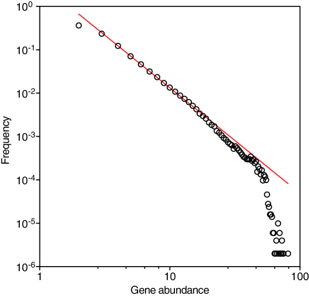
The abundance distribution of non‐redundant genes in the Red Sea community examined here. The red line shows a maximum‐likelihood estimate fit power‐law decay (F(S) ~ S – α; R ² = 0.99; P< 0.0001), with an exponent α of −2.43. An amplitude larger than 2 suggests the prevalence of rare genes in the microbiome. Further details are summarized in Supplementary Data 1. [Color figure can be viewed at wileyonlinelibrary.com]

Fig 2.

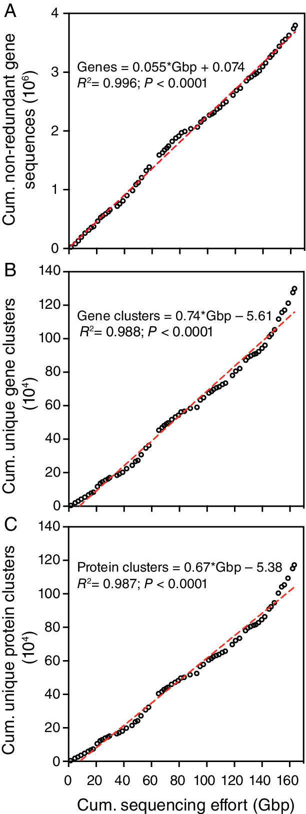
The relationship between the cumulative sequencing effort applied to metagenome samples retrieved along the 20‐day of the experiment from the different mesocosms enclosing the same initial Red Sea plankton community and the cumulative number of non‐redundant genes (A) as well as unique clusters of gene (B) and protein sequences (C) retrieved separately from each sample. The dotted red line shows the first‐order linear best‐fit regression. [Color figure can be viewed at wileyonlinelibrary.com]

The ratios of non‐redundant gene clusters and total retrieved genes indicated that the experimental perturbations steadily reduced gene sequence redundancy, particularly for samples receiving continuous nutrient additions (Fig. 3), suggesting increasing gene novelty over the sampling period. Noteworthy, as much as half of the total predicted unique genes across all samples (58± 7%; n= 65) were deduced to have a function (Supplementary Fig. S4). A similar proportion was assigned a taxonomic label (53 ± 8%), predominantly from Proteobacteria (51± 14%), Bacteroidetes (16± 9%) and Cyanobacteria (5± 6%; Supplementary Fig. S4).

Fig 3.

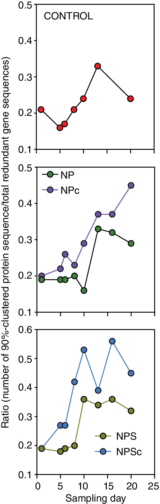
Redundancy of retrieved genes in different experimental perturbations. The ratios of the non‐redundant complete genes (90% identity over 80% of the short gene length) and the total number of predicted genes. Values are based on Supplementary Data 1. [Color figure can be viewed at wileyonlinelibrary.com]

The rank‐abundance plots of unique gene sequence clusters on the basis of KEGG Orthology (KO)—a functional orthologue of gene and protein families (Kanehisa et al., 2013)—shows a multimodal distribution of KOs (Fig. 4A), implying that rare gene families follow a distinct distribution from the abundant families. The most sequence diverse gene families—that is, KOs accompanied by distinct gene sequence clusters, averaged ~700 per sample for the top five largest gene families (Fig. 4B). Overall, the retrieved unique gene clusters across all samples (n= 65) comprised of 12 516 gene families; however, 66% of the KO entries were not represented more than five times in half of the samples, suggesting that the corresponding majority of the unique gene clusters were rare. The alpha diversity of gene families across experimental perturbations presented significantly higher (one‐way ANOVA, P< 0.0001) observed and estimated (Chao1) richness metrics in perturbations that received additional nutrients, particularly where nutrients were continuously applied relative to un‐amended controls (Fig. 3C). The top five gene families encode broad functions such as lipid metabolism, iron uptake and nucleotide biosynthesis (Fig. 4). Their discovery also increased with cumulative sequencing effort (Supplementary Fig. S5). The examination of the taxa encompassing these five top KOs indicated that much of the sequence diversity accompanying the retrieved gene families in amended perturbations resulted from changes in the abundance of gene sequence clusters originating from Alphaproteobacteria, Gammaproteobacteria and Flavobacteria, with a clear increase of Alphaproteobacteria in nitrogen, phosphate and silicate perturbations (Supplementary Fig. S6).

Fig 4.

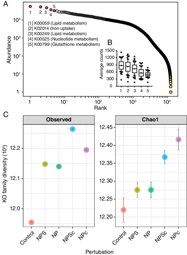
Abundance distribution and diversity of gene families. A. Rank‐abundance curve of gene families to assigned KEGG orthologues (KOs). Colour symbols indicate how dominant (red) and rare (yellow) gene families follow a multimodal distribution. B. Box plots showing the average gene sequence clusters for the top five abundant KOs (in red) encompassing three broad functional groups. The whiskers denote the 10th and the 90th percentile, while the middle horizontal line shows the median (n= 65 samples per KO). C. Alpha diversity of KOs (n = 12 516) across the treatments and the control. [Color figure can be viewed at wileyonlinelibrary.com]

Gene discovery across marine and host‐associated metagenomes

A critical question arising from the observed gene distribution pattern over the sampling period in the mesocosms experiment of the same water mass is whether the discovery of new genes (yield) increases with sequencing effort distributed over a wider geographical (latitudinal) sampling likely encompassing higher species diversity (sf. Fuhrman et al., 2008). Normalized counts of total non‐redundant genes per Tera base‐pair sequenced in the mesocosm experiment yielded 17.4 million genes Tbp⁻¹ sequenced (Table 1). The recovery of novel genes was significantly higher (one‐way ANOVA P< 0.01) in perturbations receiving continuous pulses of nitrogen, phosphate and silicate (NPSc; 12.1± 6.1× 10⁶ unique genes Tbp⁻¹) in comparison to those receiving only nitrogen and phosphate (NP and NPc; 6.3–7.3× 10⁶ unique genes Tbp⁻¹) or without any amendments (5.7× 10⁶ unique genes Tbp⁻¹; Supplementary Fig. S7).

Table 1.

The number of non‐redundant gene sequence clusters predicted in various metagenome projects exploring marine pelagic microbial communities and mammalian enteric microbiomes and corresponding yield relative to the sequencing depth applied.

			Sequenced depth (Tbp) c	Gene/protein sequences (×106) a			Yield
Project (gene catalogue)	Analytical procedures b			Redundant	Non‐redundant		(106 per Tbp)		Original data source f
		Samples			Genes d	Proteins e	Genes	Proteins
Marine
Global Ocean Sampling (GOS)	GP + GC	44	0.00625	13.6	4.5	3.9	720.0	624.0	Rusch et al. (2007)
Baltic Sea reference metagenomes	GP + GC	81	0.586	8.7	8.6	8.3	14.7	14.2	Hugerth et al. (2015)
Tara Ocean (OM‐RGC)	GP + GC	243	5.821	61.3	33.3	27.7	5.7	4.8	Sunagawa et al. (2015)
RSCK2011 g , h	AM + GP + GC	45	0.0483	2.0	1.3	1.2	26.9	24.8	Thompson et al. (2017)
Station ALOHA (HOTGC) g , i	RAM + GP + GC	103	0.638	47.3	29.6	26.1	46.4	40.9	Mende et al. (2017)
GEOTRACES program g , j	GP + GC	610	5.024	72.9	29.1	24.1	5.8	4.8	Biller et al. (2018)
MALASPINA‐Deep (MDSGC) g	RAM + GP + GC	60	0.121	11.8	6.7	6.3	55.4	52.1	Acinas et al. (2019)
MALASPINA‐profiles (MRGC) g	AM + GP + GC	116	1.714	61.6	32.7	29.0	19.1	16.9	P. Sanchez et al. in prep.
MESOCOSM g	AM + GP + GC	65	0.163	5.1	2.8	2.6	17.2	16.0	This study
Non‐marine
Human gut microbiome I g	GP + GC	124	0.577	9.7	4.1	3.8	7.1	6.6	Qin et al. (2010)
Human gut microbiome II	GP + GC	1267	6.298	121.3	18.5	16.0	2.9	2.5	Li et al. (2014)
Mouse gut microbiome k		184	0.781	22.2	2.6	n.d.	3.3	n.d.	Xiao et al. (2015)
Rat gut microbiome	GP + GC	98	0.222	26.8	7.6	6.9	34.2	31.0	Pan et al. (2018)
Pig gut microbiome k		287	1.761	62.9	7.7	n.d.	4.4	n.d.	Xaio et al. (2016)

Abbreviations: OM‐RGC, Ocean Microbial Reference Gene Catalogue; MDGC, Malaspina Deep‐Sea Gene Collection; MPRGC, Malaspina Reference Gene Catalogue; Red Sea Centre Cruise 2011; HOTGC, Hawaii Ocean Time‐series Gene Catalogue, AM, assembled; RAM, re‐assembled; GP, gene prediction; GC, gene cluster with mmseq2; n.d. not determined.

^aBased on Prodigal and retaining only complete genes. However, PGM and MGM are based on MetaGene since no assemblies were available.

^bUnless stated otherwise, all datasets were (re)analysed with the same procedures to minimize procedural artefacts.

^cBased on high‐quality read sequences except for the GEOTRACES program (raw sequencing depth) and GOS (total length of Sanger contigs ≥500 bp).

^dDefined as sequence clusters with 95% global identity over 80% of the length.

^eDefined as sequence clusters with 90% global identity over 80% of the length.

^fReported values may differ from the original reference (when reported) since re‐analyses were done in the context of this study.

^gIncludes protein‐coding genes from coassembly of unmapped reads. Details are provided in Supplementary Fig. S1.

^hBased on the assembly of data from Thompson et al. (2017) under BioProject number PRJNA289734.

ⁱBased on re‐assembly of data from Mende et al. (2017) using metaSPAdes (see Supplementary Fig. S1).

^jIncludes time‐series data from BATS and HOT, with a total of 130 metagenomes.

^kIncludes incomplete gene sequences (up to two‐thirds), with clusters defined at 95% identity over 90% of the length. The minimum length was 100 bp.

For comparison, we harmonized the metagenomic analyses (assembly, gene prediction and gene clustering) of several published metagenomes following our workflow (Supplementary Fig. S1 and Data 2–10), and used the derived gene catalogues to interrogate the link between sequencing effort and gene discovery (Table 1). Remarkably, the yield of non‐redundant genes (per Tbp sequenced) was even higher from the analysis of a regional metagenomic‐based survey along the Red Sea (RSCK2011; Thompson et al., 2017) containing 2.03 million redundant genes (n = 45 metagenomes), which produced an average (± SD) of 26± 8 million genes per Tbp (Supplementary Data 3), with no significant differences in yield by depth (one‐way ANOVA P = 0.0584; Supplementary Fig. S8). Of note, is that 65% of the retrieved protein sequence clusters in these metagenomes (total of 1.21 million at 90% identity over 80% of the length) were unmatched with Tara's 27.65‐million prodigal‐based (complete) protein clusters retrieved following a re‐analysis of Tara Ocean metagenomes (Supplementary Data 2) based on our workflow.

The recent sequencing of 60 deep‐sea (~4 km depth) metagenomes sampled by the Malaspina Circumnavigation Expedition (Acinas et al., 2019; Supplementary Data 4) supported a yield 10‐fold larger than that produced by Tara Ocean (5.7 vs. 55.4 million unique genes Tbp⁻¹) despite the 50‐fold larger sequencing effort applied in the Tara Ocean program (Table 1; Supplementary Data 2). The yield of Tara Ocean is, however, similar to that retrieved from a collection of 610 marine metagenomes sampled across space (5–1000 m) and time (Supplementary Data 5), encompassing samples from the GEOTRACES cruises (2010–2011) and the time‐series data collection from the Station ALOHA and BATS (Biller et al., 2018). The trend of higher yield, ranging from 14.7 to 46.4 million non‐redundant genes Tbp⁻¹, is also corroborated by the re‐analysis of several marine datasets conforming to our workflow (Supplementary Fig. S1): (i) the Baltic Sea reference metagenomes (BARM; n= 81) spanning both spatial and temporal dimensions (Hugerth et al., 2015), (ii) the Malaspina Circumnavigation Expedition targeting the pelagic community (Duarte, 2015, P. Sanchez et al. in prep.; Supplementary Data 6) and (iii) the prokaryotic metagenomes derived from recurrent sampling at a single location (surface to a depth of 1km) in the North Pacific Subtropical Gyre (Station ALOHA; n= 103; Supplementary Data 7; Mende et al., 2017), all supported by a much lower sequencing effort (threefold to 10‐fold lower) than that applied in the Tara Oceans program (Table 1).

The re‐analysis of host‐associated microbial metagenomics gene sequence for human (Qin et al., 2010; Li et al., 2014) and rat (Pan et al., 2018) microbiomes (Supplementary Data 8–10) together with published pig and mouse microbiome catalogues (Xiao et al., 2015, 2016) reveal a total of 2.6–18.5 million non‐redundant genes generated from 0.22 to 6.3 Tbp of high‐quality sequencing data (Table 1). Overall these enteric microbiomes support yields ranging from 2.9 to 34.4 million non‐redundant genes Tbp⁻¹ (Table 1), which is similar to the rate of gene discovery in the Tara Oceans and the GEOTRACES program (Table 1).

A significant exception to the range of gene yield discovered in Illumina‐based marine and host‐associated metagenomes reported above (2.9–55.4 million non‐redundant genes Tbp⁻¹; Table 1), is represented by the early GOS expedition, which despite a modest Sanger‐based sequencing effort of only 6.25 Gbp (Rusch et al., 2007; Yooseph et al., 2010) delivered about 4.5 million non‐redundant genes, with a corresponding yield of 725 million non‐redundant genes Tbp⁻¹. The yield is about 13–250 times larger than more recent state‐of‐the‐art metagenome‐based sequencing efforts (Table 1).

The relationship of sequencing depth to non‐redundant gene counts or the yield of genes discovered approximate a power law (Fig. 5; Supplementary Table S9); the recovery of novel genes scales as the 0.64 power of sequencing depth for marine metagenomic projects (Fig. 5A and B) and somewhat lower, 0.53, for all metagenomic biomes combined (Fig. 5B and C). However, the yield of novel genes scales inversely with increasing sequencing depth (Fig. 5B and D), showing that whereas gene discovery continues to increase with increasing sequencing effort this leads to diminishing returns on effort.

Fig 5.

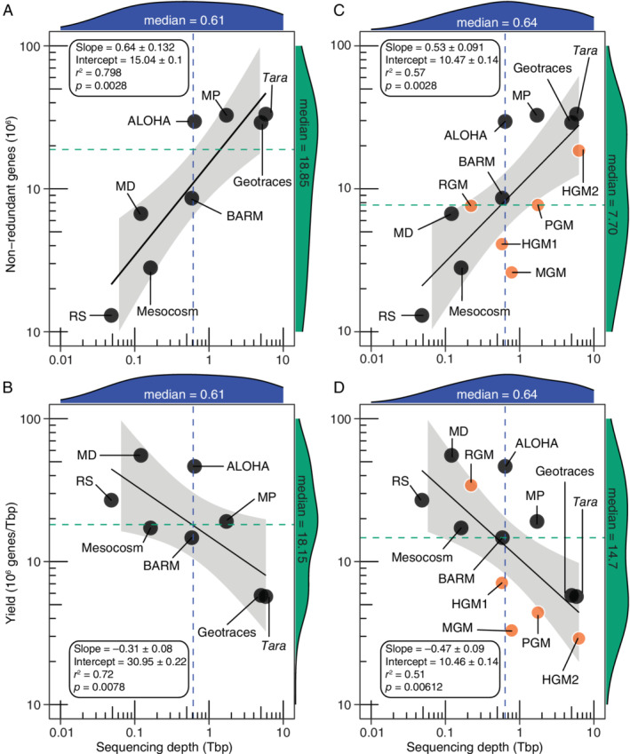
The relationship between sequencing depth and the number of non‐redundant genes or gene yield in different high‐throughput sequencing projects encompassing only marine metagenomes (A and B) or including host‐associated microbiomes (B and C). The black line indicates the log–log fit to the data (Supplementary Data 11), while the grey area shows the 95% confidence intervals for the regression curve. The distributions of the ‘x’ and ‘y’ axis values are highlighted in blue and green respectively, with corresponding medians denoted by coloured dotted lines. Black and orange circular symbols denote marine and mammalian enteric microbiomes respectively. Abbreviations: RS, Red Sea Cruise 2011; MD, Malaspina Deep; BARM, Baltic Sea reference metagenomes; MP, Malaspina Profile; HGM, human gut microbiome; PGM, pig gut microbiome; MGM, mouse gut microbiome; RGM, rat gut microbiome. Note that GOS (Table 1) was not included as it used a different sequencing technology. Additional information is provided in Supplementary Data 1–11. [Color figure can be viewed at wileyonlinelibrary.com]

Discussion

The results presented here demonstrate that the gene catalogue derived from marine microbial metagenomes is strongly dependent on sequencing effort, as reinforced by the linear increase in the number of unique genes found with cumulative sequencing effort in the Red Sea community sampled (Fig. 2). However, the relationship between sequencing effort and yield may not be unique to programs exploring the ocean microbiome.

A priori expectations would have suggested that the number of unique genes per unit sequencing effort should be lower for a single‐community analysis, such as the mesocosm studied here than when a comparable sequencing effort is distributed across the global ocean, expected to encompass a broader diversity of microbes. Yet, this was not the case, with the yield per unit sequencing effort in the Red Sea community studied here being about three times larger than that for the Tara Oceans expedition, where the 36‐fold greater total sequencing effort was distributed across the global ocean (Sunagawa et al., 2015). Possible reasons for the higher gene discovery yield of unique genes in the mesocosm experiment presented here compared with Tara Oceans include the perturbations applied, which allowed rare genes to rise above the detection limit in some treatments.

Additionally, different metagenomic analytic procedures such as the selected sequence assembler (van der Walt et al., 2017, Forouzan et al., 2018) or the gene prediction software also likely affect the quality and quantity of recovered genes (Suzek et al., 2014; Hauser et al., 2016). Also the inherent richness of rare genes in an ecosystem might confound gene discovery metrics.

The median yield of non‐redundant genes discovered for every Tera base‐pair of microbial metagenomic community DNA sequenced was 14.7 million unique genes per Tera base‐pair (Fig. 5), but varied greatly (∼3–55 × 10⁶ unique genes Tbp⁻¹; Table 1), across microbial metagenome projects using comparable next‐generation sequencing approaches encompassing a wide range of scope and targets, including projects exploring regional (e.g., Red Sea and Station ALOHA, Thompson et al., 2017, Mende et al., 2017), global expeditions (Tara Oceans, Sunagawa et al., 2015, and Malaspina, Duarte 2015, Acinas et al., 2019), and temporal and depth changes (Biller et al., 2018) in microbial diversity, as well as projects examining enteric mammalian microbiomes (Qin et al. 2010, Li et al., 2014, Pan et al., 2018, Xiao et al., 2015, 2016, 2015b; Table 1). A remarkable outlier to the gene discovery yield is represented by the early Sanger‐based GOS sequencing effort of only 6.25 Gbp (Rusch et al., 2007, Yooseph et al., 2010), with a yield that is about 13–250 times larger than more recent state‐of‐the‐art Illumina‐based metagenome sequencing efforts (Table 1). Probably, this is due to improved gene prediction associated with the higher precision and longer read lengths obtained with Sanger sequencing in the GOS expedition compared with more recent metagenome projects, all based on Illumina sequencing. In turn, this suggests the need to improve sequence length and reduce error rates in current high‐throughput sequencing technologies.

Our analysis shows that the yield of unique, non‐redundant genes in microbial metagenome sequencing projects decreases with effort, with the rate of discovery decreasing 10‐fold from projects applying limited effort to those deploying the largest sequencing effort (Fig. 5). However, new genes continue to be discovered even at projects deploying high sequencing depth, showing no evidence of saturation. This suggests, in the case of marine microbial metagenome sequencing projects, that microbial communities present high connectivity across the global ocean (Finlay, 2002), because circulation and other transport processes (e.g., long‐range air‐borne transport (Mayol et al., 2017) re‐distribute microbial communities across the ocean, while their very large population size overcomes dispersal limitation (Finlay, 2002), as indicated by relatively small differences in microbial communities across ocean basins (Sunagawa et al., 2015; Salazar et al., 2016). Our results suggest that the gene discovery yield is higher, for a given sequencing effort in the deep sea compared with the upper ocean, possibly reflecting differences in diversity and dominance patterns, biogeographic drivers, as well as global population sizes among these two ocean realms (Sunagawa et al., 2015, Salazar et al., 2016). The comparison among microbial metagenome sequencing projects also suggests that the gene discovery yield is higher, for a given sequencing depth, for host‐associated metagenomes compared with marine environments, likely reflecting the vast differences in total population sizes among these environments.

Most importantly, our results suggest that, despite being seemingly phenomenal compared with the sequencing depth possible just a decade ago, the sequencing effort applied by modern metagenomic projects is still very far from that necessary to completely retrieve the enormous pool of unique genes present in the rare microbial biosphere. This suggests that those genes belonging to the tail of the Pareto distribution are beyond the capabilities of current metagenome sequencing projects and can only be retrieved if a perturbation, such as the nutrient additions conducted here, allows them to become more abundant. Indeed, recent analyses of power laws describing the relationship between sampling effort and the number of species retrieved in microbial communities have extrapolated the global number of microbial species on Earth from about a few million to 1 trillion (10¹²) microbial species (Locey and Lennon, 2016), largely resulting from the pool of rare microbes concealed within the rare biosphere (Pedros‐Alio, 2012).

The OM‐RGC, describing unique genes retrieved from planktonic microbes, contained a phenomenal 40 million non‐redundant gene sequence clusters (Sunagawa et al., 2015). Yet, this likely represents only the tip of the iceberg of microbial gene diversity in the ocean. Sequencing efforts at least an order of magnitude greater per sample than those used to‐date applied along global and regional expeditions, time‐series sampling or perturbation experiments are required to retrieve the large pool of unreported genes, and hence novel functions, that still remain untapped in the vast ocean.

Experimental procedures

Experimental design and procedures

A total of 10 mesocosm bags, each containing 8000 L (depth: 2.5 m) were situated in the harbour of King Abdullah University Science and Technology (KAUST), Thuwal, Saudi Arabia (Lat: 22.304°N; Long: 39.103°E). The bags were filled with harbour seawater and subjected to one of five different nutrient treatments (each with two biological replicates) as depicted below:

1. Control mesocosm: No addition of nutrients

2. Nitrate (NaNO₃) and phosphate (H₂NaPO₄P·H₂O) (NP) addition on day 1.

3. Nitrate (NaNO₃), phosphate (H₂NaPO₄P·H₂O) and silicate (Na₂SiO₃·9H₂O) (NPS) addition on day 1.

4. Nitrate (NaNO₃) and phosphate (H₂NaPO₄P·H₂O) (NPc) addition each day for 2 weeks.

5. Nitrate (NaNO₃), phosphate (H₂NaPO₄P·H₂O) and silicate (Na₂SiO₃·9H₂O) (NPSc) addition each day for 2 weeks.

The concentrations of the nutrients in the experiments were for the single additions: 16, 1 and 39 μM for nitrate, phosphate and silicate respectively. For the continuous treatments, they were 2, 0.12 and 3.75 μM for nitrate, phosphate and silicate respectively. The ratios were adapted from those published by Wyman et al. (2000).

Sample collection and sequencing procedures

Samples were collected at solar noon daily over a 20‐day period lasting from the 27th January to the 15th February 2013. Twenty litres of seawater was collected in a Niskin bottle at a depth of 1 m. The water (4 L per replicate) was prefiltered to remove debris and zooplankton, and immediately filtered through a 0.22 μm CellTrap filter (MemTeq) using a peristaltic pump at low speed (70 rpm) so as to avoid the destruction of delicate cells. The cell concentrate was eluted in 1.2 ml of filtered mesocosm water (from the same mesocosm) and flash‐frozen in liquid nitrogen. The samples collected were then selected for sequencing among the resulting set of 80 samples to target specific aspects of the bloom (e.g., representing pre‐bloom, peak bloom and bloom decline), based on flow cytometry data. As these stages were not observed in all mesocosms, a total of 71 samples were selected for sequencing. Since six samples failed to sequence, the final sample set consisted of 65 metagenomes. DNA was extracted using a phenol:chloroform:isopropanol and bead‐beating protocol as described in detail by Pearman et al. (2015). Paired‐end sequencing libraries (100 × 2 bp) were prepared using the NEBNext Ultra DNA kit (#E7370L) following the manufacturer's protocol. Six samples per lane were subsequently sequenced on an Illumina HighSeq 2000 sequencer at the KAUST Biosciences Corelab (BCL). The total raw sequencing effort equals 185 Gbp, averaging 2.9 ± 1.2 Gbp (mean ± SD) for each of the 65 samples (Supplementary Data 1).

Metagenomic assembly and protein‐coding gene prediction

Raw read sequences were quality filtered and trimmed using Trimmomatic v0.32 (Bolger et al., 2014) to remove adapter sequences and leading and trailing bases with a quality score below 20 and reads with an average per base quality of 20 over a 4‐bp window. This pre‐processing step also included a mapping‐based step to remove the phiX reads (an internal standard) using BBmap v37.44 (http://jgi.doe.gov/data-and-tools/bbtools/). Unless otherwise stated all data generated in this study followed the workflow described in Supplementary Fig. S1. Post‐trimming quality was assessed with FASTQC (http://www.bioinformatics.babraham.ac.uk/projects/fastqc/).

For the mesocosm experiments, the total sequencing effort after this procedure was 163.4 Gbp, averaging 2.5 ± 1.1 Gbp (n = 65 samples; Supplementary Data 1). This was distributed across the five different treatments as follows: CONTROLs (26.5 Gbp or 16.2% of total; n = 12), NP pulse additions (42.4 Gbp or 26%; n = 15), NP continuous additions (34.4 Gbp or 21.1%; n = 13), NPS pulse additions (28.4 Gbp or 17.4%; n = 11) and NPS continuous additions (31.6 Gbp or 19.3%; n = 14). Another 89.8 Gbp dataset from the Red Sea, which is already published (RSCK2011; BioProject number PRJNA289734) (Thompson et al., 2017), comprising 45 Red Sea metagenomes sampled across different water column depths (from surface to 1000 m), averaging 2.0 ± 0.4 Gbp per sample (Supplementary Data 1) was analysed similarly. The final high‐quality (paired‐end) data used for downstream steps for the RSCK2011 comprised 48.3 Gbp (n = 45; average of 1.07 ± 0.22 Gbp per sample; Supplementary Data 2).

The resulting high‐quality reads for each dataset were independently assembled with metaSPAdes v3.9.0 (Nurk et al., 2017), which was ranked as the ‘best’ in recent evaluations of metagenomic assemblers in terms of contig lengths and reduced miss‐assemblies (van der Walt et al., 2017; Forouzan et al., 2018), employing the error‐correction mode, the preset metagenomic options and a kmer range of 21–127 (Supplementary Fig. S1). Each metagenomic assembly was quality controlled for minimum contig length of 500 bp, generating sample‐specific assemblies that were individually mapped against the corresponding error‐corrected reads aimed at producing additional contigs from all unassembled reads. Read mapping was conducted using BBmap v37.44 (https://jgi.doe.gov/data-and-tools/bbtools/) based on the default settings and the option ‘pairedonly = t’. The resultant unmapped paired‐end reads from all samples were subsequently co‐assembled with MegaHit v1.1.2 (Li et al., 2015), using the same kmer cutoff range as above and setting the minimum contig length to 500 bp. This metagenomic workflow was also applied to the recently published water column metagenomes (n = 45) from the Red Sea (RSCK2011) (Thompson et al., 2017). In additions, two datasets from the Malaspina Circumnavigation Expedition (Duarte, 2015), namely MALASPINA DEEP (n = 60) (Acinas et al., 2019) and the unpublished MALASPINA PROFILE (n = 116; P. Sanchez et al. in prep.), as well as the publicly available metagenomic reads from station ALOHA (n = 103) (Mende et al., 2017) retrieved from the NCBI short read archive under the Bioproject number PRJNA352737 were similarly pre‐processed and assembled (Supplementary Fig. S1).

To improve our sampling size, the published assemblies of seven additional datasets were also included, encompassing marine and host‐associated metagenomes downloaded from various repositories (Supplementary Data 3–10), including: (i) the Sanger‐based contigs of the GOS Expedition (Rusch et al., 2007) retrieved from the NCBI (https://www.ncbi.nlm.nih.gov/books/NBK6855/); (ii) the SOAPdenovo‐based assemblies of Tara Ocean microbiome program (n = 242) (Sunagawa et al., 2015) retrieved from the European Nucleotide Archive database (https://www.ebi.ac.uk/ena/about/tara-oceans-assemblies); (iii) the SPAdes‐based microbial metagenomes (n = 610) sampled across space and time from the GEOTRACES cruises and two long‐term sampling sites (HOTS and BATS) (Biller et al., 2018) retrieved from the iMicrobe database under project numbers 277, 271 and 276 respectively (http://datacommons.cyverse.org/browse/iplant/home/shared/imicrobe/projects/); (iv) the megahit‐based co‐assembled contigs from the BARM database (n = 81 metagenomes) encompassing 37 time‐series datasets from the Linnaeus Microbial Observatory (Hugerth et al., 2015), 30 transect samples from the EU‐BONUS BLUEPRINT project and 24 redoxcline samples from the Boknis Eck station downloaded from FigShare (https://doi.org/10.6084/m9.figshare.c.3831631); (v) the SOAPdenovo‐based assemblies of the human gut microbiome (HGM) study of 124 individuals (Qin et al., 2010) was obtained from the dedicated repository (http://www.bork.embl.de/~arumugam/Qin_et_al_2010/); (vi) the integrated microbiome of 1267 HGM samples (Li et al., 2014) retrieved from the GigaScience database, GigaDB (http://gigadb.org/dataset/view/id/100064/File_sort/type_id), and (vii) the recent Sprague–Dawley rat gut metagenomic assemblies (n = 98 samples; Pan et al., 2018) retrieved, also from GigaDB (http://gigadb.org/dataset/100440). The analysis of these datasets included gene prediction with prodigal (for complete genes only) and gene/protein clustering with mmseq as shown Fig. S1.

For two additional host‐associated microbiome datasets (also based on the SOAPdenovo assembler), no assemblies were available. Accordingly, only the published gene catalogues and corresponding sequencing depths are reported here, including the mouse (n = 184 samples) and pig (n = 287 samples) gut microbiome projects (Xiao et al., 2015, 2016). The reported gene statistics (Table 1) for these two datasets are based on the prediction of open reading frames (ORFs) using MetaGene2 and GeneMark software respectively, with the clustering of ORFs done at a global sequence identity of 95% and an overlap of 90% for the shorter sequence using BLAT21.

With the assemblies at hand, contigs shorter than 500 bp were discarded prior to gene prediction. Putative protein‐coding genes were predicted from the size‐filtered contigs using the program Prodigal v 2.6.3 (Hyatt et al., 2010) in the metagenomic mode (‐p meta), retaining only genes that were predicted to be complete (default minimum size of 90 bp). Crucially, this workflow deviates from the one applied in the majority of the published gene catalogues that result in a large proportion of partial (in‐complete) genes (Qin et al., 2010; Xiao et al., 2015, 2016). For instance, a gene catalogue of the HGM predicted using the gene caller MetaGene revealed that nearly two‐thirds of the genes were incomplete (Qin et al., 2010). Indeed, a comparison of the gene catalogue that includes partial genes for the mesocosm datasets studied here (Supplementary Data 1) reveals a twofold difference in the number of non‐redundant gene clusters when incorporating partial genes in the catalogues. In turn, this emphasizes that the in‐depth comparison of gene catalogues requires similar metagenomic procedures and that, at a minimum, only complete genes are considered (i.e., genes with defined codon boundaries), preferably with the same gene caller (we used Prodigal).

The general statistics for these de novo (re)assembled metagenomes and published assemblies used in this study are provided in Supplementary Data 1–10. Unless mentioned otherwise, values for protein‐coding sequences refer to predicted complete gene sequences (or the corresponding protein sequences).

Use of a complementary approach that classifies contigs as being eukaryotic or prokaryotic based on the sequence signature (using EukRep, West et al., 2018) revealed that only 3% of the assembled bases in the entire dataset are potentially eukaryotic. However, gene catalogues refer to prokaryotic genes, as prokaryotic gene prediction programs are not suitable for predicting eukaryotic genes (West et al., 2018), largely because of differences in gene structure, with eukaryotic gene prediction algorithms relying on transcriptomic evidence (Mathé et al., 2002; Lomsadze et al., 2018), which is absent from our data sets. Indeed, there is no method to predict genes in eukaryotic sequences available for application in metagenomic mode (assuming mixed populations). Current eukaryotic gene predictors assume the sequence signature is from a single organism, which would lead to erroneous results.

Generation of gene and protein sequence catalogues

The redundant gene (nucleotide) sequences from individual samples or in combination with the redundant genes from the co‐assemblies of unmapped reads, where applicable (Supplementary Data 1–7), were reduced into non‐redundant gene clusters with mmeqs2 v4.6.1 (Hauser et al., 2016) based on the ‘easy‐linclust’ workflow, applying the default settings (including bidirectional coverage ‘‐‐cov‐mode 0’ and greedy clustering ‘‐‐cluster‐mode 0’), but considering the following options for global sequence identity (‐‐min‐seq‐id 0.95) and sequence length overlap of the shorter sequence (‐c 0.80). Similarly, the corresponding protein sequences were also clustered using a global sequence identity cutoff of 90% and 80% overlap, consistent with the sequence coverage concept of UniRef protein families (Suzek et al., 2014). Indeed, the applied global identity thresholds together with the 80% length overlap allows maintaining the intra‐cluster molecular function consistency of protein sequences (Suzek et al., 2014), which lends itself to the discovery of novel protein families, as exemplified in our study (sf. Figures 3 and 4).

Protein family shared with Tara Ocean catalogue

The catalogue of non‐redundant protein sequence clusters from the mesocosm (2.63 million) and the Red Sea's water column (RSCK2011; 1.21 million) metagenomes were compared against the Tara's 27.65‐million prodigal‐based (complete) protein clusters retrieved based on our workflow using mmseq2 (Hauser et al., 2016). Comparisons were done using the ‘search’ module, applying a minimum global protein sequence identity of 90% and a minimum sequence length overlap of 80%.

Rank abundance analysis of gene families in the mesocosm

A rank abundance curve of gene abundance was generated using the matrix of gene redundancy generated from mmseq2 (Hauser et al., 2016), containing the gene sequence catalogue from individual experiments (excluding the co‐assembled dataset). Clusters were sorted by an abundance from the highest to lowest, and the data were visualized on a logarithmic plot of gene copies versus frequency (Fig. 1).

Prediction of sample‐specific (unique) genes

We employed two procedures to generate unique gene and protein sequences retrieved in every sample sequenced (excluding the co‐assembled dataset) relative to the others. First, we produced representative sequence clusters using mmseq2 as described above. This step yielded a total of 1 902 457 and 1 751 030 gene and protein sequence clusters respectively out of 3.8 million predicted protein‐coding genes (Supplementary Data 1). The resultant matrices of gene and protein sequence clusters were subsequently parsed based on the sequence‐to‐mapping information to score for presence–absence of genes and protein sequences across samples, so that, a gene/protein was deduced unique if it occurred only in a single sample (out of the 65 metagenomes). These results were then used to build cumulative plots of sequencing depth versus the number of unique genes or proteins retrieved (Fig. 2B and C; Supplementary Fig. S3).

The second approach was tailored to account for sequencing depth of the genes by including the co‐assembled dataset (Supplementary Fig. S1) containing 1 288 709 putative protein‐coding genes in constructing the gene catalogue (as above) and by applying a conservative mapping rate of reads per gene cluster for defining gene presence/absence in samples. Briefly, the high‐quality reads generated from the 65 metagenomes were mapped against a catalogue of 2.83 million non‐redundant gene with BBmap (https://jgi.doe.gov/data-and-tools/bbtools/). BBmap was performed using the following parameters: nodisk = t rpkm = $fpkm ambig = toss idfilter = 0.9 tossbrokenreads. The resultant read counts per gene across all samples were subsequently normalized to account for differences in sequencing efforts among the samples with eXpress v1.5.0 (Suzek et al., 2014), resulting in a common metric of reads per million normalized abundance (RPM), commonly known as Transcript Per Million. We then used this coverage normalized gene dataset to create a binary matrix of gene presence/absence based on a conserved minimum RPM cutoff of 0.25 (equivalent to 2500 reads mapped per gene). The ‘best’ RPM value of 0.25 was deduced from the analysis of the effect of different RPM cutoffs on the recovery of unique genes in different samples—that is, by examining the average counts of unique genes recovered at different RPM cutoffs (Supplementary Fig. S3). In our normalized datasets, RPM values range from 0 to ~11 000, representing a gene that is completely absent in a sample and one that is extremely highly represented.

These analyses indicated, as expected, that increasingly higher RPM cutoff values (above 0.25) impacted the recovery of unique genes—that is, higher mapping rates are associated with more prevalent genes (Supplementary Fig. S9). However, RPM values ranging from 0.005 to 0.25 (corresponding to 50–2500 reads mapped per gene) were not statistically different regarding the average counts of unique genes recovered (one‐way ANOVA, P > 0.05; Supplementary Fig. S9). The minimum RPM value (of 0.25) with no significant difference in the global detection of unique genes is similar to the mean RPM of 0.24 for the whole dataset. It is noteworthy that the application of similar cutoffs on Tara Ocean's published matrix of normalized gene abundance (downloaded June 2018; http://ocean-microbiome.embl.de/companion.html) indicated no significant differences (Mann–Whitney U test, P > 0.5) in the retrieval of unique genes among the 243 samples—whether an RPM of 0.0001 or 0.25 was applied (Supplementary Fig. S10). However, it is likely that the functional diversity accompanying the corresponding gene families differs significantly, but this was not interrogated beyond the present goal. Accordingly, we applied an RPM cutoff of 0.25 as the conservative minimum coverage to designate the uniqueness of genes in a sample. Subsequently, we generated a presence–absence scoring matrix, with samples fulfilling this criterion receiving a score of one, indicating the presence of a gene (out of 2.83 million genes). In turn, a gene was defined as unique if it occurred only in a single sample based on this matrix.

On this basis, a total of 137 482 sample‐specific (complete) unique genes were predicted, averaging (±SD) 2115 ± 1598 genes per sample (n = 65). This implies that roughly 7.7% of the non‐redundant genes were unique only to one sample. Only 2142 genes (out of 5.1 million non‐redundant genes) were predicted as conserved across all 65 samples, including the control and the different nutrient perturbations. Counts of complete redundant genes across samples significantly positively correlated with counts that included partial genes (R ² = 0.997, P < 0.0001). However, counts of unique gene clusters from complete genes only (based on the 0.25 RPM criterion above) were ineffectively paired with counts of unique gene clusters that included partial genes (R ² = 0.019, P = 0.88). Together with the highly significant differences (Two‐tailed paired t‐test P < 0.0001; n = 65) in the average (±SD) counts of unique gene clusters obtained from complete versus complete plus partial gene catalogues (Supplementary Data 1 ) suggests a strong effect of partial gene sequences on gene diversity, and in turn, gene discovery. Based on the complete gene catalogue, the resulting cumulative count of unique genes recovered at increasing sampling effort was plotted against the cumulative sequencing depth of the same sampling over time (Supplementary Fig. S11). The data show that unique gene discovery is still at a linear phase even when applying a conserved sequencing depth to retrieve novel genes.

Curve fitting

Non‐linear regression analysis was conducted in R v3.6.0 environment (https://www.R-project.org/). Linear and non‐linear (power, exponential and logistic) models were fitted using the ‘curvefit’ function in the ‘REAT’ package v3.02 (Wieland, 2019). The goodness of fit was tested using the one‐way ANOVA comparing linear, logistic, power and exponential models of distribution (Supplementary Data 11). Graphs were plotted using ‘ggplot2’ v3.3.0 and ‘ggstatsplot’ v0.5.0 packages (Wickham, 2016; Patil, 2018).

Functional annotation of gene catalogues

Functional annotation of gene catalogues (non‐redundant representative complete gene sequences) was conducted in the Automatic Annotation of Microbial Genomes pipeline (Alam et al., 2013) hosted at KAUST's Dragon Metagenomic Analysis Platform (http://www.cbrc.kaust.edu.sa/dmap). Briefly, the protein‐coding sequence (CDS) is each catalogue were uploaded as input and annotated in the metagenomic mode using the following workflow. Briefly, gene annotations are performed by parallel Blast comparisons (minimum blast score of 40), first against the complete UniProt KnowledgeBase (downloaded March 2017) and second against the KEGG database (downloaded March 2018) with defined KOs groups (Kanehisa et al., 2013). The UniProt KnowledgeBase (UKB) is mainly used to obtain generic functional and taxonomic assignments, while KEGG is used to link predicted gene functions to KEGG pathways and modules. In addition, InterProScan is used to obtain gene ontology assignments and to detect protein families and signature domains from InterPro, Prosite, Pfam (Bateman et al., 2004) and TIGRfam (Haft et al., 2003) databases. The fraction of genes with predicted functions were then calculated based on the combined annotation of these databases.

Significant differences between the average count of genes retrieved at different RPM cutoff thresholds were tested by conducting a one‐way ANOVA using GraphPad Prism v8.0 (GraphPad Software, Inc.). Multiple comparisons for controlling the false discovery rate (α = 0.05) were conducted with the Benjamini–Hochberg's two‐stage step‐up method (Benjamini et al., 2006). The richness of unique gene families (KOs) across perturbations was calculated using the phyloseq R package (McMurdie and Holmes, 2013).

Metagenomes from the MESOCOSMS experiment are deposited at NCBI under BioProject number PRJNA395437.

Supporting information

Fig. S1 Metagenomic analysis work‐flow employed in this study.

Fig. S2. The relationship between the cumulative sequencing effort applied to metagenome samples retrieved from mesocosms subject to different treatments (control, NP: single nitrogen and phosphorus additions, NPc: continuous nitrogen and phosphorus additions; NPS: single nitrogen, phosphorus and silicon additions; and NPSc: continuous nitrogen, phosphorus and silicon additions) along the 20‐day of the experiment, and the cumulative number of non‐redundant genes discovered. The red dotted lines indicate a first‐order linear best‐fit regression.

Fig. S3. The relationship between the cumulative sequencing effort applied to metagenome samples retrieved from mesocosms subject to different treatments (as in Fig. S2) and the cumulative number of unique gene (a) and protein (b) sequence clusters retrieved. The red dotted lines indicate a first‐order linear best‐fit regression.

Fig. S4. The annotation and taxonomic breakdown of the unique gene sequences retrieved different perturbations and the control.

Fig. S5. The relationship between the cumulative sequencing effort applied to metagenome samples retrieved from mesocosms subject to different treatments (as in Fig. S2) and the cumulative number of unique gene families retrieved for the top five largest KEGG orthologue (KOs) groups. The red dotted lines indicate a first‐order linear best‐fit regression.

Fig. S6. The taxonomic breakdown of gene sequence clusters corresponding to the top five largest KOs in different perturbations and the control. Source data are provided as a Source Data file.

Fig. S7. The yield of novel genes per Tbp of sequenced data in different perturbations and the control. Pairwise multiple comparisons with one‐way analysis of variance (ANOVA) (post hoc adjusted P < 0.05) reveal significantly higher average yields in perturbations receiving continuous amendments of nitrogen, phosphorus, and silicate (NPSc).

Fig. S8. The yield of non‐redundant genes per Tbp of sequenced data across different depths in Red Sea metagenomes (RSCK2011). Data are the mean (± SD) of 11 to 15 sampling points in each experiment (Supplementary Data 3). No significant difference in yield by depth was detected (one‐way ANOVA post hoc adjusted P > 0.05) for the Red Sea metagenomes (n = 45; ≤ 0.1 to ≤1.2 μm size‐fractioned samples; 10–500 m depth). However, the red dotted line shows that the average yield is six‐folds higher than the yield from the Tara Ocean (n = 242; ≤ 0.22 to ≤3 μm size‐fractioned samples; 5–1000 m depth) demarcated with a blue dotted line.

Fig. S9. The relationship between mapping rates per gene and the average number of unique genes recovered across metagenomes. (Upper panel) Unique genes are defined as those that are only present in a single sample after applying a given read per million normalized abundance (RPM) cutoff. The circular symbols indicate the mean (± SEM) of unique gene counts from the 65 samples. Pairwise multiple comparisons with one‐way ANOVA (post hoc adjusted P < 0.05) were used to identify significant differences between the average numbers of recovered genes at different RPM cutoffs. Different letter codes above symbols indicate a significant difference between data. (Lower panel) Shows the proportion of unique genes at each RPM cutoff that could be assigned a putative function and those predicted as hypotheticals.

Fig. S10. Mapping coverage (RPM cutoff) effects on gene discovery across Tara Ocean metagenomic datasets. The original matrix of gene abundance (8) based on the reads per million normalized abundance (RPM) metric was used. Although the number of unique genes was significantly different between the data set obtained by the applied cutoff 0.0001 in the original data (n = 243) and our conserved value of 0.25 RPM, no significant differences in the average count of unique genes between these two cutoffs were detected even by depth (Mann–Whitney U‐test P > 0.5).

Fig. S11. The relationship between the cumulative sequencing effort applied to metagenome samples retrieved from mesocosms subject to different treatments at an RPM cutoff of 0.25 and the cumulative number of unique gene and protein sequence clusters retrieved. The circular symbols indicate plots of the raw data, while the blue solid line and red dotted lines indicate a first‐order linear best‐fit regression and the 95% confidence interval for the fitted line respectively. Source data are provided as a Source Data file.

Data 1. The general stats for metagenomic samples in the different mesocosm experiments, receiving different nutrient treatments (perturbations).

Data 2. General stats for the assembled 45 Red Sea metagenomes.

Data 3. General stats for predicted genes in Tara Ocean assemblies, including twelve metagenomes sampled from the Red Sea highlighted in yellow.

Data 4. General stats for the assembled 60 MALASPINA DEEP metagenomes.

Data 5. General stats for predicted genes in the published GEOTRACES assemblies.

Data 6. General stats for the assembled 116 MALASPINA PROFILE metagenomes.

Data 7. General stats for the assembled 103 ALOHA metagenomes (Mende et al. 2017).

Data 8. General stats for predicted genes in Human Gut Microbiome project 1 assemblies.

Data 9. General stats for predicted genes in Human Gut Microbiome project 2 assemblies.

Data 10. General stats for predicted genes in Rat Gut Microbiome project assemblies.

Data 11. Curve fitting results for sequencing depth versus number of non‐redundant genes or gene yield.

References

- Acinas, S.G. , Sánchez, P. , Salazar, G. , Cornejo‐Castillo, F.M. , Sebastián, M. , Logares, R. , Sunagawa, S. , Hingamp, P. , Ogata, H. , Lima‐Mendez, G. , Roux, S. , González, J.M. , Arrieta, J.M. , Alam, I.S. , Kamau, A. , Bowler, C. , Raes, J. , Pesant, S. , Bork, P. , Agustí, S. , Gojobori, T. , Bajic, V. , Vaqué, D. , Sullivan, M.B. , Pedrós‐Alió, C. , Massana, R. , Duarte, C.M. , and Gasol, J.M. 2019. Metabolic architecture of the deep ocean microbiome, bioRxiv 635680
- Alam, I. , Antunes, A. , Kamau, A.A. , Kalkatawi, M. , Stingl, U. , and Bajic, V.B. (2013) INDIGO – INtegrated Data Warehouse of MIcrobial GenOmes with examples from the Red Sea extremophiles. PLoS One 8: e82210. [DOI] [PMC free article] [PubMed] [Google Scholar]
- Bateman, A. , Coin, L. , Durbin, R. , Finn, R.D. , Hollich, V. , Griffiths‐Jones, S. , et al (2004) The Pfam protein families database. Nucleic Acids Res 28: 263–266. [DOI] [PMC free article] [PubMed] [Google Scholar]
- Benjamini, Y. , Krieger, A.M. , and Yekutieli, D. (2006) Adaptive linear step‐up procedures that control the false discovery rate. Biometrika 93: 491–507. [Google Scholar]
- Biller, S.J. , Berube, P.M. , Dooley, K. , Williams, M. , Satinsky, B.M. , Hackl, T. , et al (2018) Marine microbial metagenomes sampled across space and time. Sci Data 5: 180176. [DOI] [PMC free article] [PubMed] [Google Scholar]
- Bolger, A.M. , Lohse, M. , and Usadel, B. (2014) Trimmomatic: a flexible trimmer for Illumina sequence data. Bioinformatics 30: 2114–2120. [DOI] [PMC free article] [PubMed] [Google Scholar]
- Duarte, C.M. (2015) Seafaring in the 21st century: The Malaspina 2010 Circumnavigation Expedition. Limnol Oceanogr Bull 24: 11–14. [Google Scholar]
- Finlay, B.J. (2002) Global dispersal of free‐living microbial eukaryote species. Science 296: 1061–1063. [DOI] [PubMed] [Google Scholar]
- Forouzan, E. , Shariati, P. , Mousavi Maleki, M.S. , Karkhane, A.A. , and Yakhchali, B. (2018) Practical evaluation of 11 de novo assemblers in metagenome assembly. J Microbiol Methods 151: 99–105. [DOI] [PubMed] [Google Scholar]
- Fuhrman, J.A. , Steele, J.A. , Hewson, I. , Schwalbach, M.S. , Brown, M.V. , Green, J.L. , and Brown, J.H. (2008) A latitudinal diversity gradient in planktonic marine bacteria. Proc Natl Acad Sci U S A 105: 7774–7778. [DOI] [PMC free article] [PubMed] [Google Scholar]
- Gianoulis, T.A. , Raes, J. , Patel, P.V. , Bjornson, R. , Korbel, J.O. , Letunic, I. , et al (2009) Quantifying environmental adaptation of metabolic pathways in metagenomics. Proc Natl Acad Sci U S A 106: 1374–1379. [DOI] [PMC free article] [PubMed] [Google Scholar]
- Haft, D.H. , Selengut, J.D. , and White, O. (2003) The TIGRFAMs database of protein families. Nucleic Acids Res 31: 371–373. [DOI] [PMC free article] [PubMed] [Google Scholar]
- Hauser, M. , Steinegger, M. , and Söding, J. (2016) MMseqs software suite for fast and deep clustering and searching of large protein sequence sets. Bioinformatics 32: 1323–1330. [DOI] [PubMed] [Google Scholar]
- Hugerth, L.W. , Larsson, J. , Alneberg, J. , Lindh, M.V. , Legrand, C. , Pinhassi, J. , and Andersson, A.F. (2015) Metagenome‐assembled genomes uncover a global brackish microbiome. Genome Biol 16: 279. [DOI] [PMC free article] [PubMed] [Google Scholar]
- Hyatt, D. , Chen, G.L. , LoCascio, P.F. , Land, M.L. , Larimer, F.W. , and Hauser, L.J. (2010) Prodigal: prokaryotic gene recognition and translation initiation site identification. BMC Bioinformatics 11: 119. [DOI] [PMC free article] [PubMed] [Google Scholar]
- Kanehisa, M. , Goto, S. , Sato, Y. , Kawashima, M. , Furumichi, M. , and Tanabe, M. (2013) Data, information, knowledge and principle: back to metabolism in KEGG. Nucleic Acids Res 42: D199–D205. [DOI] [PMC free article] [PubMed] [Google Scholar]
- Karsenti, E. , Acinas, S.G. , Bork, P. , Bowler, C. , De Vargas, C. , Raes, J. , et al (2011) A holistic approach to marine eco‐systems biology. PLoS Biol 9: e1001177. [DOI] [PMC free article] [PubMed] [Google Scholar]
- Li, D. , Liu, C.‐M. , Luo, R. , Sadakane, K. , and Lam, T.‐W. (2015) MEGAHIT: an ultra‐fast single‐node solution for large and complex metagenomics assembly via succinct de Bruijn graph. Bioinformatics 31: 1674–1676. [DOI] [PubMed] [Google Scholar]
- Li, J. , Jia, H. , Cai, X. , Zhong, H. , Feng, Q. , Sunagawa, S. , et al (2014) An integrated catalog of reference genes in the human gut microbiome. Nat Biotechnol 32: 834–841. [DOI] [PubMed] [Google Scholar]
- Locey, K.J. , and Lennon, J.T. (2016) Scaling laws predict global microbial diversity. Proc Natl Acad Sci U S A 113: 5970–5975. [DOI] [PMC free article] [PubMed] [Google Scholar]
- Lomsadze, A. , Gemayel, K. , Tang, S. , and Borodovsky, M. (2018) Modeling leaderless transcription and atypical genes results in more accurate gene prediction in prokaryotes. Genome Res 28: 1079–1089. [DOI] [PMC free article] [PubMed] [Google Scholar]
- Mathé, C. , Sagot, M.‐F. , Schiex, T. , and Rouzé, P. (2002) Current methods of gene prediction, their strengths and weaknesses. Nucleic Acids Res 30: 4103–4117. [DOI] [PMC free article] [PubMed] [Google Scholar]
- Mayol, E. , Arrieta, J.M. , Jiménez, M.A. , Martínez‐Asensio, A. , Garcias‐Bonet, N. , Dachs, J. , et al (2017) Long‐range transport of airborne microbes over the global tropical and subtropical ocean. Nat Commun 8: 201. [DOI] [PMC free article] [PubMed] [Google Scholar]
- McMurdie, P.J. , and Holmes, S. (2013) phyloseq: an R package for reproducible interactive analysis and graphics of microbiome census data. PLoS One 8: e61217. [DOI] [PMC free article] [PubMed] [Google Scholar]
- Mende, D.R. , Bryant, J.A. , Aylward, F.O. , Eppley, J.M. , Nielsen, T. , Karl, D.M. , and DeLong, E.F. (2017) Environmental drivers of a microbial genomic transition zone in the ocean's interior. Nat Microbiol 2: 1367–1373. [DOI] [PubMed] [Google Scholar]
- Nurk, S. , Meleshko, D. , Korobeynikov, A. , and Pevzner, P.A. (2017) metaSPAdes: a new versatile metagenomic assembler. Genome Res 27: 824–834. [DOI] [PMC free article] [PubMed] [Google Scholar]
- Pan, H. , Guo, R. , Zhu, J. , Wang, Q. , Ju, Y. , Xie, Y. , et al (2018) A gene catalogue of the Sprague‐Dawley rat gut metagenome. GigaScience 7: giy055. [DOI] [PMC free article] [PubMed] [Google Scholar]
- Patil, I. (2018) ggstatsplot: ‘ggplot2’ Based Plots with Statistical details. CRAN. doi: 10.5281/zenodo.2074621. [DOI]
- Pearman, J.K. , Casas, L. , Merle, T. , Michell, C. , and Irigoien, X. (2015) Bacterial and protist community changes during a phytoplankton bloom. Limnol Oceanogr 61: 198–213. [Google Scholar]
- Pedros‐Alio, C. (2012) The rare bacterial biosphere. Ann Rev Mar Sci 4: 449–466. [DOI] [PubMed] [Google Scholar]
- Qin, J. , Li, R. , Raes, J. , Arumugam, M. , Burgdorf, K.S. , Manichanh, C. , et al (2010) A human gut microbial gene catalogue established by metagenomic sequencing. Nature 464: 59–65. [DOI] [PMC free article] [PubMed] [Google Scholar]
- Rusch, D.B. , Halpern, A.L. , Sutton, G. , Heidelberg, K.B. , Williamson, S. , Yooseph, S. , et al (2007) The Sorcerer II global ocean Sampling Expedition: Northwest Atlantic through eastern tropical Pacific. PLoS Biol 5: e77. [DOI] [PMC free article] [PubMed] [Google Scholar]
- Salazar, G. , Cornejo‐Castillo, F.M. , Benítez‐Barrios, V. , Fraile‐Nuez, E. , Álvarez‐Salgado, X.A. , Duarte, C.M. , et al (2016) Global diversity and biogeography of deep‐sea pelagic prokaryotes. ISME J 10: 596–608. [DOI] [PMC free article] [PubMed] [Google Scholar]
- Sunagawa, S. , Coelho, L.P. , Chaffron, S. , Kultima, J.R. , Labadie, K. , Salazar, G. , et al (2015) Structure and function of the global ocean microbiome. Science 348: 1261359. [DOI] [PubMed] [Google Scholar]
- Suzek, B.E. , Wang, Y. , Huang, H. , McGarvey, P.B. , Wu, C.H. , and UniProt Consortium . (2014) UniRef clusters: a comprehensive and scalable alternative for improving sequence similarity searches. Bioinformatics 31: 926–932. [DOI] [PMC free article] [PubMed] [Google Scholar]
- Thompson, L.R. , Williams, G.J. , Haroon, M.F. , Shibl, A. , Larsen, P. , Shorenstein, J. , et al (2017) Metagenomic covariation along densely sampled environmental gradients in the Red Sea. ISME J 11: 138–151. [DOI] [PMC free article] [PubMed] [Google Scholar]
- van der Walt, A.J. , Van Goethem, M.W. , Ramond, J.B. , Makhalanyane, T.P. , Reva, O. , and Cowan, D.A. (2017) Assembling metagenomes, one community at a time. BMC Genomics 18: 521. [DOI] [PMC free article] [PubMed] [Google Scholar]
- Vidondo, B. , Prairie, Y.T. , Blanco, J.M. , and Duarte, C.M. (1997) Some aspects of the analysis of size spectra in aquatic ecology. Limnol Oceanogr 42: 184–192. [Google Scholar]
- West, P.T. , Probst, A.J. , Grigoriev, I.V. , Thomas, B.C. , and Banfield, J.F. (2018) Genome‐reconstruction for eukaryotes from complex natural microbial communities. Genome Res 28: 569–580. [DOI] [PMC free article] [PubMed] [Google Scholar]
- Whitman, W.B. , Coleman, D.C. , and Wiebe, W.J. (1998) Prokaryotes: the unseen majority. Proc Natl Acad Sci U S A 95: 6578–6583. [DOI] [PMC free article] [PubMed] [Google Scholar]
- Wickham, H. (2016) gplot: Elegant Graphics for Data Analysis. New York: Springer‐Verlag. [Google Scholar]
- Wieland, T. (2019) “REAT”: a regional economic analysis toolbox for R. Region 6: R1–R57. [Google Scholar]
- Wyman, M. , Davies, J.T. , Crawford, D.W. , and Purdie, D.A. (2000) Molecular and physiological responses of two classes of marine chromophytic phytoplankton (diatoms and prymnesiophytes) during the development of nutrient‐stimulated blooms. Appl Environ Microbiol 66: 2349–2357. [DOI] [PMC free article] [PubMed] [Google Scholar]
- Xiao, L. , Estellé, J. , Kiilerich, P. , Ramayo‐Caldas, Y. , Xia, Z. , Feng, Q. , Liang, S. , et al. (2016). A reference gene catalogue of the pig gut microbiome. Nature Microbiology, 1: 1–66. 10.1038/nmicrobiol.2016.161. [DOI] [PubMed] [Google Scholar]
- Xiao, L. , Feng, Q. , Liang, S. , Sonne, S.B. , Xia, Z. , Qiu, X. , et al (2015). A catalog of the mouse gut metagenome. Nature Biotechnology 33: 1103–1108. 10.1038/nbt.3353. [DOI] [PubMed] [Google Scholar]
- Xiao, L. , Feng, Q. , Liang, S. , Sonne, S.B. , Xia, Z. , Qiu, X. , et al (2015b) A reference gene catalogue of the pig gut microbiome. Nat Microbiol 1: 1–6. [DOI] [PubMed] [Google Scholar]
- Yooseph, S. , Nealson, K.H. , Rusch, D.B. , McCrow, J.P. , Dupont, C.L. , Kim, M. , et al (2010) Genomic and functional adaptation in surface ocean planktonic prokaryotes. Nature 468: 60–66. [DOI] [PubMed] [Google Scholar]
- Yooseph, S. , Sutton, G. , Rusch, D.B. , Halpern, A.L. , Williamson, S.J. , Remington, K. , et al (2007) The Sorcerer II Global Ocean Sampling Expedition: expanding the universe of protein families. PLoS Biol 5: e16. [DOI] [PMC free article] [PubMed] [Google Scholar]
Associated Data
This section collects any data citations, data availability statements, or supplementary materials included in this article.
Supplementary Materials