Abstract
With the development of multi-model neuroimaging technology and gene detection technology, the efforts of integrating multi-model imaging genetics data to explore the virulence factors of schizophrenia (SZ) are still limited. To address this issue, we propose a novel algorithm called group sparse of joint non-negative matrix factorization on orthogonal subspace (GJNMFO). Our algorithm fuses single nucleotide polymorphism (SNP) data, function magnetic resonance imaging (fMRI) data and epigenetic factors (DNA methylation) by projecting three-model data into a common basis matrix and three different coefficient matrices to identify risk genes, epigenetic factors and abnormal brain regions associated with SZ. Specifically, we introduce orthogonal constraints on the basis matrix to discard unimportant features in the row of coefficient matrices. Since imaging genetics data have rich group information, we draw into group sparse on three coefficient matrices to make the extracted features more accurate. Both the simulated and real Mind Clinical Imaging Consortium (MCIC) datasets are performed to validate our approach. Simulation results show that our algorithm works better than other competing methods. Through the experiments of MCIC datasets, GJNMFO reveals a set of risk genes, epigenetic factors and abnormal brain functional regions, which have been verified to be both statistically and biologically significant.
Index Terms—: Group Sparse, Imaging Genetics, Joint Non-negative Matrix Factorization, Orthogonal Subspace, Schizophrenia
1. Introduction
IMAGING genetics is an emerging field in brain research [1, 2], which uses brain imaging technology evaluate the influence of genes on individuals, and discusses how genes affect the neural structure, the brain function and the resulting pathology of the nervous system[3–5]. Studying on correlation between genetic variables and imaging variables will facilitate mental disease research like schizophrenia (SZ).
Canonical Correlation Analysis (CCA)[6] is a typical method which is used to find the relationship between genetic and brain imaging data. However, high dimensionality problem featured by high dimension variables and limited sample size in both data sets remains to be a challenge for quantitative analysis. To overcome this issue, feature selection is often integrated in current computational models. For instance, Wright and Parkhomenko et al.[7, 8] built sparse canonical correlation analysis (SCCA), in which L1-norm aims to extract significant features through sparse canonical variables and L2-norm is used to relieve overfitting problems. Since SCCA doesn’t consider the prior information of data, several researchers developed SCCA by adding prior information as constraint conditions. Lin However, a CCA-based model can only find a pair of canonical correlation variables (i.e. one of the modules) at the same time. In order to obtain the second pair, the third pair or even all the canonical correlation variables, we need dimensionality problem featured by high dimension variables and limited sample size in both data sets remains to be a challenge for quantitative analysis. To overcome this issue, feature selection is often integrated in current computational models. For instance, Wright and et al. [9] proposed group sparse CCA(GSCCA), in which the group information of data was considered. Du et al.[10] proposed structure CCA algorithm, in which the spatial structure information of imaging genetics datasets was employed. Moreover, to take advantage of the complementary information of multiple datasets, three or more datasets need to be integrated, Witten et al.[8] proposed sparse Multi-modal CCA (SMCCA) to find the maximum correlation among three or more datasets. Recently, Hu et al.[11] developed an adaptive SMCCA as an extension of the two-module SCCA model.
However, a CCA-based model can only find a pair of canonical correlation variables (i.e.one of the modules) at the same time. In order to obtain the second pair, the third pair or even all the canonical correlation variables, we need to gradually build new CCA model based on the results of the previous step, leading the model to be more complex and time-consuming. The extended model of the non-negative matrix factorization (NMF) algorithm can help to overcome these limitations.
Non-negative matrix factorization [12, 13] is a low-dimensionality reduction approach which has been widely used to analyze imaging genetics datasets since it is useful for learning parts-based representation. NMF decomposes the non-negative object matrix into the non-negative basis matrix and the coefficient matrix. Considering the group and structure information as prior, Kim et al.[14] proposed a group sparse non-negative matrix factorization (GSNMF) algorithm. GSNMF imposed L1,q-norm to realize sparse representation at the level of groups[15]. On the basis of NMF, Zhang et al.[16] proposed joint non-negative matrix factorization (JNMF) algorithm which projected multi-modal datasets into a common space for multiple data fusion. Since JNMF hadn’t taken into account data prior information, and Wang et al.[13] proposed group sparse joint non-negative matrix factorization (GSJNMF) by combing JNMF and GSJNMF. In these works, each row of the coefficient matrix is equivalent to a canonical correlation variable in CCA model. That is, JNMF and GSJNMF can identify multiple sets of canonical correlation variables simultaneously. However, this NMF-based approach did not consider the correlation between basis vectors, which may lead to extract unimportant features from coefficient matrix.
To this end, we propose a novel model named group sparse of joint non-negative matrix factorization on orthogonal subspace (GJNMFO). GJNMFO enforces both orthogonal and group sparse constraints in matrix decomposition and projects multi-modal data into a low-dimensional orthogonal space. Compared to the previous NMF-based methods, our model has the following advantages. First, we use the idea of joint non-negative matrix to fuse multi-modal imaging genetics data, which can make full use of the complementary information between multi-modal data. Second, GJNMFO projects multi-modal data into a common basis matrix. We employ orthogonal constraint on basis matrix to reduce the correlation between the basis vectors, which helps discard unimportant features in the rows of coefficient matrix. Third, since the imaging genetics datasets have rich group information (i.e., brain voxel can be group by brain functional regions, SNP sites and DNA methylation CpG sites can be grouped by gene), we draw into group sparse constraint on coefficient matrices to make the extracted genetic variables and imaging variables more accurate.
We validate GJNMFO algorithm with both the simulated and real datasets. Simulation results show that our algorithm can identify significant features in multi-modal dataset, and outperform than other existing algorithms, i.e., GSJNMF and JNMF. Results by using the Mind Clinical Imaging Consortium (MCIC) data demonstrate that our algorithm find the reveals a set of risk genes (PLA2G4A, INSIG2, etc.), epigenetic factors (C10orf26, MTERF, etc.) and abnormal brain regions (Hippocampus, Occipital_Inf, etc.) closely related to schizophrenia.
The rest of this paper is organized as follows. In Section II, we propose GJNMFO algorithm and give the numerical optimization, significance estimation and parameter selection strategy. In Section III, we compare the performance of GJNMFO, GSJNMF and JNMF on the simulated data, then use GJNMFO algorithm to analyze the SNP, DNA methylation and fMRI datasets of SZ. Some concluding remarks are given in Section IV.
2. Materials and Methods
2.1. NMF and Extension
NMF has been widely used in data mining and pattern recognition [16–20]. The basic description of NMF model is: given a non-negative matrix , we aim to find two low-rank non-negative matrices and such that
| (1) |
where m and n are the number of samples and features, respectively. r is the number of components, and ∥·∥F is the Frobenius norm. Here, W and H are called basis matrix and coefficient matrix, respectively. As shown in Eq. (1), X can be represented by a linear combination of r basis components with relevant coefficients.
Although NMF algorithm performed well on the low-dimensional representation via single matrix decomposition, there was an urgent need to find the connections of two or multiple matrices. Joint non-negative matrix factorization (JNMF) was then proposed to address this issue by decomposing multiple input matrices into one common shared basis matrix and multiple corresponding coefficient matrices. In this way, JNMF can find the association among multi-modal datasets via different coefficient vectors under the common basis vector. As shown in Fig.1, JNMF decomposes multiple input datasets into one common shared basis matrix and multiple different coefficient matrices.
Fig. 1.
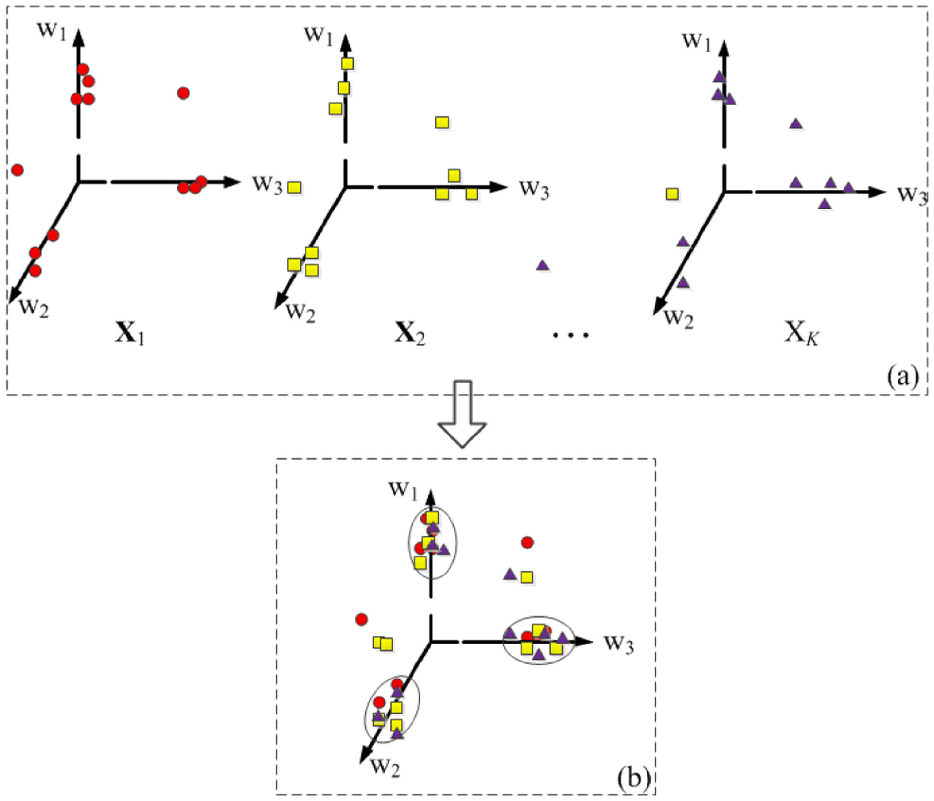
JNMF decomposes the multimodal imaging genetics data into a new common orthogonal space. w1, w2, and w3 represent basis vectors. Triangles, squares and circles represent data of different modalities. In Fig.1a, the original data X1, X2, ⋯, XK are projected into the respective basis vectors. In Fig.1b, the multimodal data XK is projected into the same set of basis vectors.
Denote , , …, as input matrices, JNMF can be formulated as:
| (2) |
where m and ni represent the number of samples and features in Xi (i=1, 2, 3), respectively. On the basis of JNMF, Wang et al.[13] proposed group sparse joint non-negative matrix factorization (GSJNMF) by considering prior group information as constrain imposed on JNMF.
However, these JNMF-based algorithms did not take the correlation between columns of basis matrix into account, so there may be a linear correlation between the basis vectors. This may cause these JNMF-based algorithms extract the insignificant features from coefficient matrix. To this end, we propose a novel algorithm, named group sparse joint non-negative matrix factorization on orthogonal subspace (GJNMFO).
2.2. The Proposed Method
GJNMFO is a JNMF-based method, aiming to discover the potential relationship among multi-modal datasets. Considering the group information of each dataset, i.e. the brain imaging is divided into different ROIs, and the nucleotides belongs to different genes, we use group information as constraint to the coefficient matrices. Meanwhile, in order to ensure that the basis matrix is full-rank, we impose orthogonal constraint on the basis matrix. Specifically, for the i-th modal dataset, the features can be divided into di group by utilizing the prior information. Then we employ GJNMFO to decompose the multi-model input data Xi to one common shared basis matrix W and multiple corresponding coefficient matrices Hi, as shown in Fig. 2. Since Hi is composed by features which also contain the same group information as input, here we impose group sparse constraint on Hi to extract the significant group of features. In addition, for the common matrix W, we use WTW-I as orthogonal constraint guarantee full-rank and remove the linear correlation of components. Thus, the objective function of GJNMFO is formulated as follows:
| (3) |
where λi and γ are regularization parameters. γ ≥ 0 controls orthogonality of the vectors in W (i.e. The larger the γ, the more orthogonal the basis vector is.[21]) and λi control sparsity at the group level. For the input matrix Xi, assuming that ni features consist of di disjoint groups, we have ςi:
| (4) |
where is the column index set which belongs to J-th group in Xi. The group information contained in the features of the original data Xi is projected to the coefficient matrix Hi by GJNMFO algorithm.
Fig. 2.
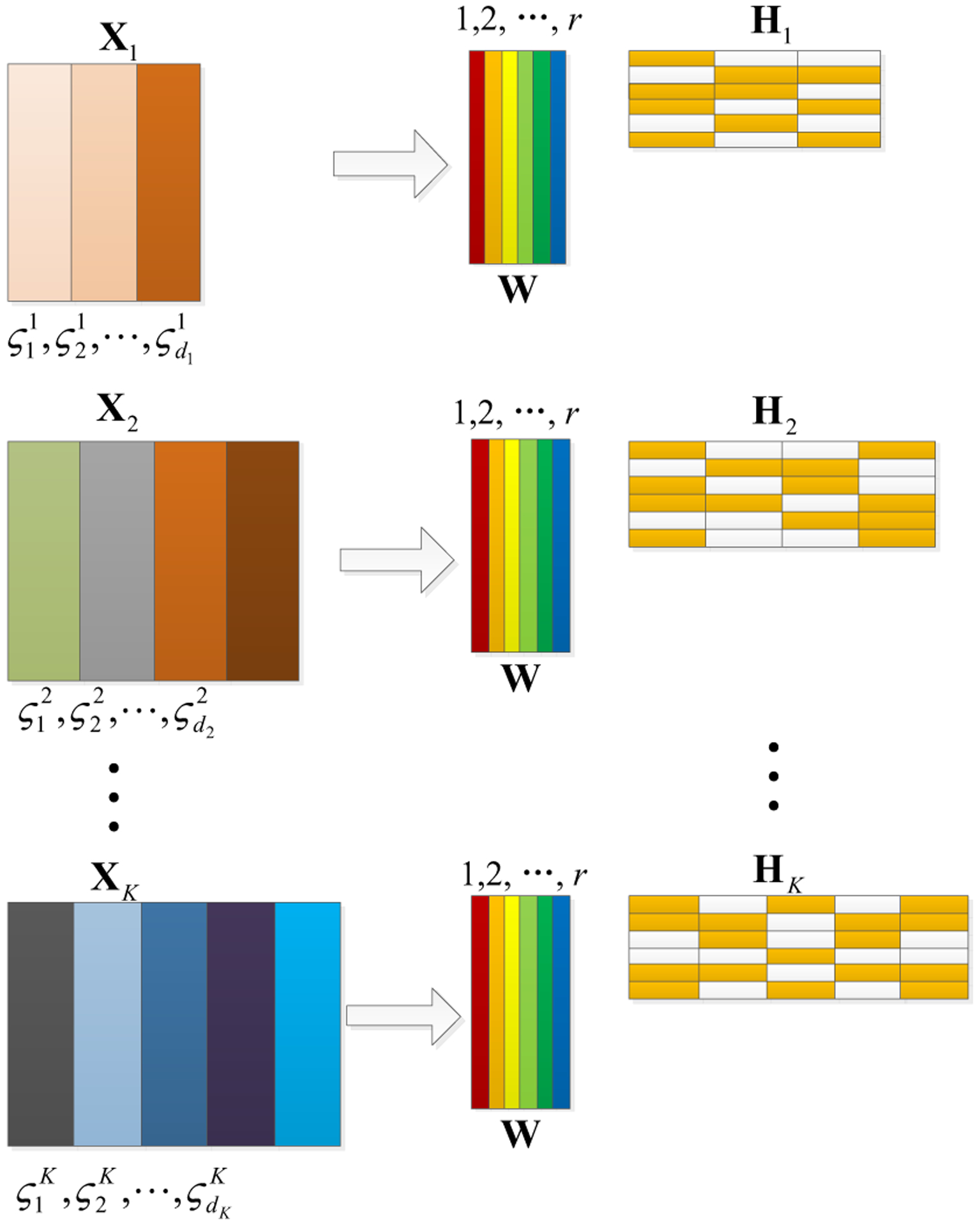
Schematic illustrating our method. Our method projects the multi-modal imaging genetics data into a common matrix and different coefficient matrices. The features of the original data XK can be divided into dK groups, which are . The yellow and white in H1, H2, …, Hk represent non-zero and zero respectively.
For non-negative coefficient matrix , we assume that each row index set of H is divided into d disjoint groups according to X, and each group has |ςJ | elements respectively. The group norm of the J-th group in the j-th row is defined as:
| (5) |
where ςJ is the column index set that belongs to the J-th group in the j-th row of H. Then the group norm of matrix coefficient H can be defined in the following manner:
| (6) |
It should be noted that is the L1,2-norm ∥·∥1,2 if one row of Hj. belongs to a single group. Since the number of elements in each group in the coefficient matrix is different, calculating the group norm by Eq. (6) will have different sparsity for each element in Hi. In order to overcome this problem, we add the size of each group in Eq. (6) to form the final group norm, i.e. ‖Hi‖ς is defined in the following manner:
| (7) |
where is the number of elements in J-th group in Hi.
It is straightforward to show that problem (3) is non-convex and it is hard to solve it directly. We propose an efficient algorithm based on ALS approach. Let and be the Lagrange multipliers to constraint W ≥ 0 and Hi > 0 respectively. Then the Lagrange function L has the following expression:
| (8) |
where tr(·) is trace operation. Taking the partial derivative to W and Hi (i=1, 2, …, K) of L, we then obtain:
| (9) |
| (10) |
According to the Karush-Kuhn-Tucker conditions[22] Ψ pqWpq = 0 and (Φi)pq(Hi)pq = 0, we get the following equations for Wpq and (Hi)pq.
Then we can get the update equations as follows:
| (11) |
| (12) |
where
| (13) |
The iteration termination condition for GJNMFO is ∣ Lk+1 − Lk ∣/∣Lk+1 ∣ ≤ τ , where τ is a predefined tolerance error, we generally set τ = 10−6. Lk+1 and Lk are the (k + 1) − th and k − th reconstruction errors, respectively. The k-th reconstruction error Lk is defined as follows:
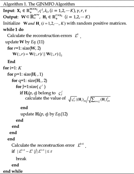
Where W(k) and represent W and Hi obtained at the k-th iteration, respectively. The pseudocode of GJNMFO algorithm is shown in Algorithm 1.
As GJNMFO projects multi-model data into a common orthogonal space W, we use each basis component in W as the ‘building block’ to explore the correlation of different datasets. In original NMF, the maximum value of each column in Hi is usually used to define variable’s membership[23]. In this way, each variable can belong to one and only one module. However, some variable may not be active in any module or may be active in multiple modules with multiple functions [16]. Based on this problem, we calculate the z-score of each element in each row of H1, H2, H3 by the following formula.
| (14) |
where μu and σu represent the mean and variance of the u-th row in Hi, respectively. The Q-th basis vector wQ is only related to the Q-th row of Hi (i=1, 2, …, K, Q=1, 2, …, r). We select element zuv> T to form index set of features , where is the sub-index set of feature selected from the Q-th row in Hi and T is a predefined threshold. Each variable set SQ can be regarded as a module (or building block).
3. Experiments and Results
The purpose of GJNMFO algorithm is to explore the biomarkers of schizophrenia, i.e. to identify risk genes, epigenetic factors and abnormal brain functional regions. In this paper, we use X1, X2, and X3 to represent SNP, fMRI, and DNA methylation datasets, respectively. We use GJNMFO to decompose X1, X2, and X3 to obtain r (where r is the numbers of components) modules. We adopt permutation test to evaluate which modules are significant.
3.1. Significance Estimation
For the Q-th module , assume that , and where ag bt ce are column vectors selected from X1, X2, and X3 according to , and , respectively. Based on the above assumption, the mean of correlations among the three types of datasets in a module can be expressed as follows:
| (15) |
For a given matrix CQ, we randomly change the order of the row vectors of the matrices AQ and BQ in Q-th module, and repeat this process Δ times. For each permutation, ρ* is used as the null hypothesis of mean correlation, and is the new mean correlation coefficient calculated by Eq. (15) after the row of permutation matrix AQ and BQ. The significance of the test statistic can be estimated by
| (16) |
Where |·| denotes the number of times . If the P-value is less than 0.05, we consider this module is significant.
3.2. Parameter Selection
In GJNMFO, we tune five parameters r, γ, λ1, λ2 and λ3. Since determining r is still a challenging problem (if r is too small may lead to a large tolerance error and hinder the extraction of hidden skeletons in data. if r is too large, the purpose of low-rank decomposition of matrix cannot be achieved, which is also not conducive to mining the hidden skeleton in data), we generally set r≈0.1* min(m, n1, n2, n3). γ is used to control the orthogonality of the column vectors in the basis matrix W. If the value of γ is too large, the basis vectors are too sparse, so that the tolerance error of the objective function Eq. (3) is large. If the value of γ is too small, the correlation between the basis vectors cannot be reduced. We selected a variable γ based on the number of iterations. It can be defined as follows:
| (17) |
where k is the number of iterations and γ0 = 0.1. A smaller ξ causes faster changes of γk and vice versa. The value range of ξ is 0 ≤ ξ < 1. According to experience, we usually make ξ = 0.1. λ1, λ2 and λ3 are used to constrain ςi in the coefficient matrix Hi (i=1, 2, 3) respectively. According to Ref. [13], the value range of λ1, λ2 and λ3 is . We use the grid search method to find the optimal value of the objective function Eq. (3). Finally, when | Lk+1 − Lk |/| Lk+1 | ≤ τ and the reconstruction error is the smallest, the corresponding λ1, λ2 and λ3 are the optimal parameters of the model.
3.3. Simulations
In order to test the effectiveness of GJNMFO algorithm, we construct four sets of simulated datasets and then compare the performance of JNMF, GSJNMF and GJNMFO. Finally, we analyze the SNP, fMRI and DNA methylation datasets to identify risk genetic variables, epigenetic factors and abnormal brain ROIs.
3.3.1. Construction the Simulated Data
Owing to the group number and the feature number in each group may not equal, so we generate 4 cases of simulation datasets based on the different group structure information. In each case, there are 3 matrices Xi (i=1, 2, 3) consisting of several disjoint groups. The details of the number of groups and features in 4 cases are shown in Table I.
TABLE I.
The Number of Groups and Features in Four Cases
| case 1 | case 2 | case3 | case4 | |
|---|---|---|---|---|
| Number of groups in Xi | 1 | 1 | 0 | 0 |
| Number of features in each group | 1 | 0 | 1 | 0 |
Statements that ‘1’ means equal and ‘0’ mean unequal. For example, in case 2, ‘1’ indicates that the number of groups among X1, X2, and X3 is equal, and ‘0’ indicates that the features number of each group in Xi (i=1, 2, 3) is not equal.
To imitate group structure information, features of the same group are generated by the same seed vector. Assuming that a group contains n features, it can be defined as follows:
| (18) |
where is a seed vector, and it is generated from a standard normal distribution. is known as Gaussian noise. ℓ denotes a variable that represents the noise level. According to Eq. (18), we construct the simulated data of the four cases. The details are shown in table II.
TABLE II.
The Column Index Set of Correlated Modules in Each Case
| Dataset | column index set | |||||||
|---|---|---|---|---|---|---|---|---|
| casel | case2 | case3 | case4 | |||||
| module1 | module2 | module1 | module2 | module1 | module2 | module1 | module2 | |
| X1 | 1~20 | 41~60 | 1~15 | 21~29 | 1~20 | 41~60 | 1~100 | 101~230 |
| X2 | 41~60 | 1~20 | 31~41 | 1~11 | 21~40 | 1~20 | 281~390 | 1~80 |
| X3 | 81~100 | 61~80 | 50~55 | 7~15 | 81~100 | 121~140 | 410~590 | 171~290 |
The numbers (i.e. 1~20, 41~60, 1~15 etc.) in table II indicate the column index of the feature in Xi. In each case, there are two correlated modules in the three data matrices. For example, in module1 of case1, 1~20 features of X1, 41~60 features of X2, and 81~100 features of X3 are generated by the same seed vector. In simulated data, the row of Xi (i=1,2,3) in each case represents a sample, the column of Xi represents a feature. The sample number m of Xi is equal in all cases, and in this study, m = 40.
To ensure that the Xi (i=1, 2, 3) satisfies the non-negative constraint, we pre-process the datasets in the following four steps. Firstly, we use the z-score method to standardize each column of data, so that the mean value of each column is 0 and the variance is 1. Secondly, we use F(x)=x-min(x) to make each column non-negative, where x is a column vector. Thirdly, we use the L2-norm to the unit each column vector of Xi. Fourthly, we scale all the Xi (i=1, 2, 3) matrices so that their Frobenius norms are equal. Through this step Xi (i=1, 2, 3) have the same value level. It should be noted that the above four steps are linear transformations. Next, we use the above simulation data to verify the performance of JNMF, GSJNMF and GJNMFO.
3.3.2. Analysis of Simulation Result
In our simulation data, there are two correlated modules in each case. Since the basis matrix W has a total of 5 column vectors, there are a total of 5 modules. We calculate the z-score (Eq.14) in each module and then select two modules which are the closest to the ground truth as the experimental result. Furthermore, in order to compare the performance of GJNMFO, GSJNMF and JNMF algorithms at different noise levels, we let ℓ=0.5, 1, 1.5 to construct the simulated data, respectively. Fig. 3 shows the z-score of features obtained by GJNMFO, GSJNMF and JNMF three algorithms in case1.
Fig. 3.
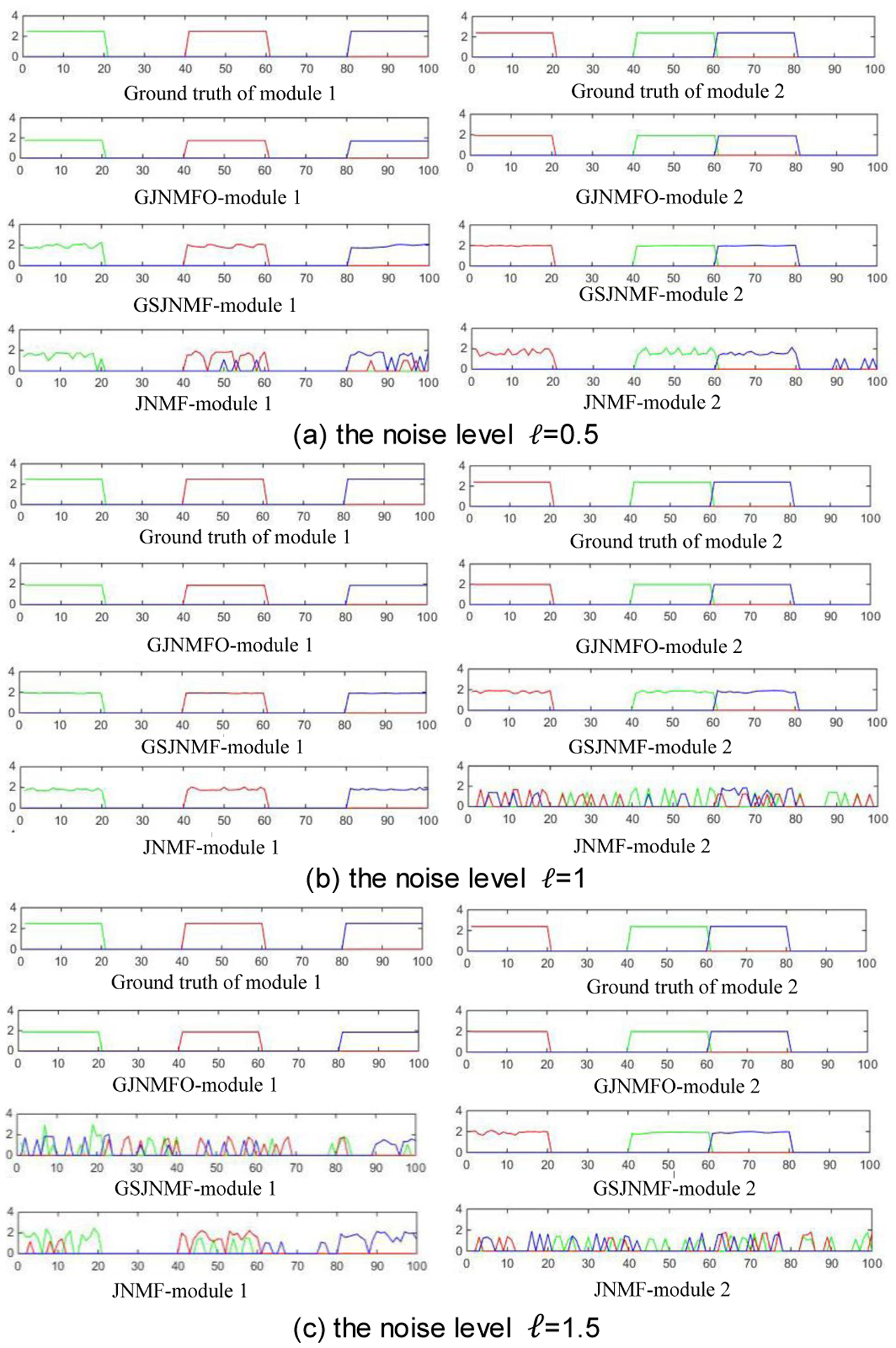
Z-score of features obtained by GJNMFO, GSJNMF and JNMF three algorithms in case1. (a), (b), and (c) are z-score of features obtained by three algorithms at a noise level of 0.5, 1, and 1.5, respectively. Ground truth represents the real z-score of the features.
In Fig. 3, Ground truth represents the real z-score of the features in case1, and the color of the line represents the datasets Hi (i=1, 2, 3), where green, red and blue color represent H1, H2 and H3 correspondingly.
From Fig. 3(a) we can see, the z-score of GJNMFO in module 1 and module 2 are very close to ground truth and the line are very flat; The z-score of GSJNMF in module 1 and module 2 are close to the ground truth, but the line becomes fluctuant. Even though JNMF can identify most of the significant features, it unfortunately mixes some unrelated features in module 1 and module 2, making the line becomes more fluctuant.
When the noise level is ℓ = 1 (As it shows in Fig.3(b)), although both GJNMFO and GSJNMF can identify the significant features in module 1 and module 2, GJNMFO line is flat in two modules, and GSJNMF’s line becomes fluctuant due to the incorporation of unrelated features in module 2. JNMF has not recognized the significant features in module 2.
When noise level is ℓ = 1.5 (As it shows in Fig.3(c)), GJNMFO can accurately identify the meaningful features in module 1 and module 2, and the line is still flat. GSJNMF’s module 1 is not flat because some unimportant features are selected. JNMF has not recognized the significant features whether it is module 1 or module 2.
We present the simulation results for case2, case3, and case4 in Appendix A. By comparing the simulation results in the four cases, we can conclude that GJNMFO has better anti-noise performance compared with the state-of-the-art algorithm GSJNMF and JNMF when the level of noise is high.
To analyze the reasons for the performance degradation of GJNMFO, GSJNMF, and JNMF when the noise level increases, we draw the correlation between any two columns in the basis matrix of the three algorithms at different noise levels. The results are shown in Fig. 4.
Fig. 4.
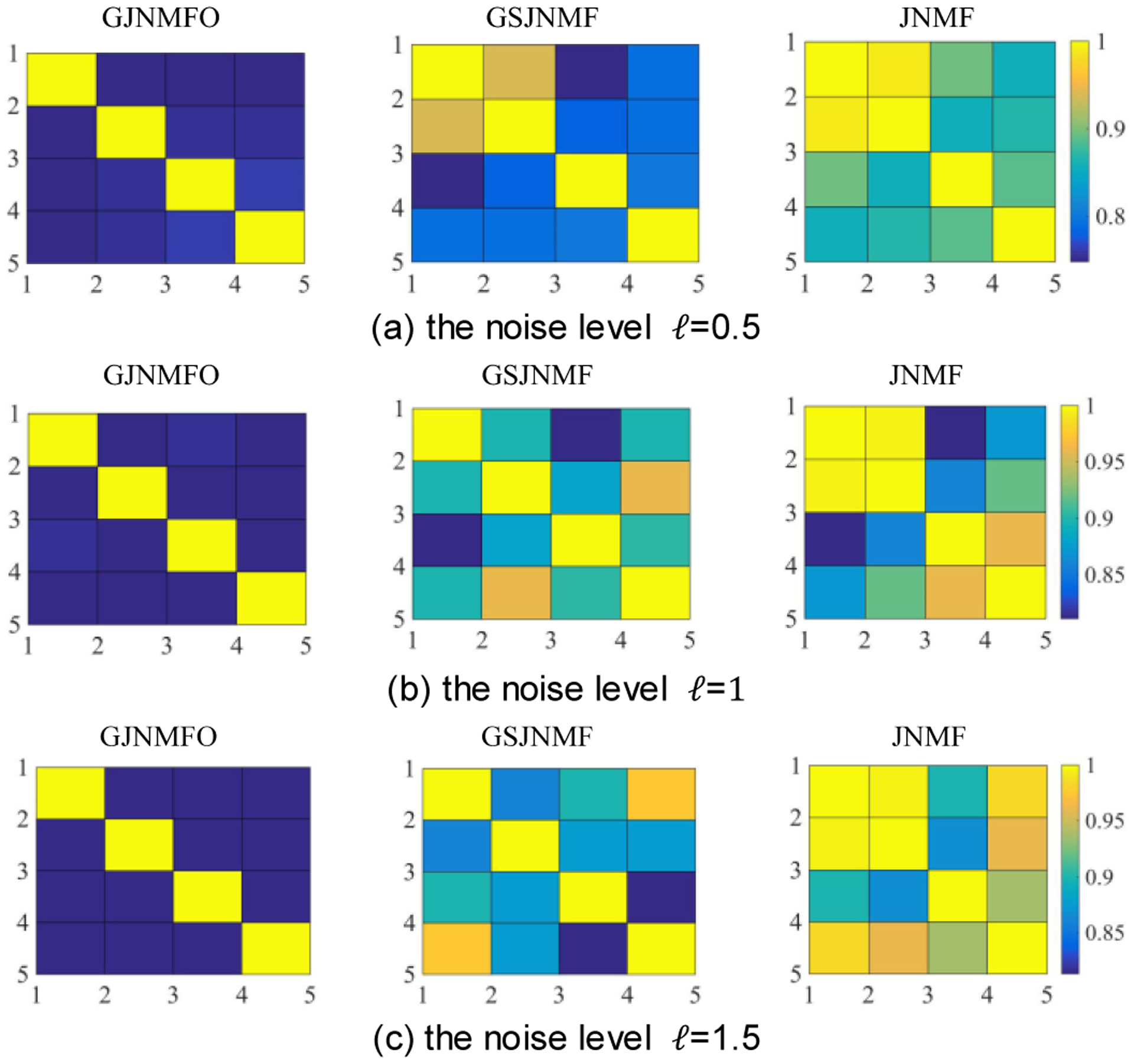
The correlations between any two columns in the basis matrix of GJNMFO, GSJNMF and JNMF at different noise levels in case1.
As can be seen from Fig. 4, with the increase of noise level, the correlation between the basis vectors of GJNMFO is always low, while the correlation between the basis vectors of GJNMFO and JNMF increases with the increase of noise level. When the correlation between basis vectors in GSJNMF and JNMF increases, some unrelated features are mixed and the ability to identify significant features is lost. For example, unrelated features are mixed in JNMF-module 2 in Fig. 3(a). Since too many unrelated features are mixed, some meaningful feature in GSJNMF-module 1 of Fig. 3(c) can’t to be identified. However, GJNMFO algorithm overcomes above problem by imposing orthogonal constraints to the basis matrix, which makes GJNMFO algorithm has good anti-noise performance.
In order to further discuss the effect of introducing orthogonal constraints on the basis matrix, we have generated a new set of simulated data , , and . Where m represents sample size, n1, n2 and n3 represent features size, and we set m = 80, n1 = 100, n2 = 120 and n3 = 140 in this paper. Specifically, the generation procedure of X1, X2 and X3 are similar to that in Ref. [10] [24] with the following four steps: 1) we generate vectors u1, u2 and u3 with lengths of 100, 120, and 140, respectively. Let u1 be a vector with 1st~10th elements as 1, 51st~60th elements as 2, 71st~90th elements as 2, and other elements as 0. We use the group information in u1 as a priori, i.e. ς = {{1, ⋯ 10}, {11, ⋯, 50}, {51, ⋯, 60}, {61, ⋯, 70}, {71, ⋯, 90}, {91, ⋯, 100}}. Let u2 be a vector with 1st~20th elements as 1, 31st~40th elements as 2, 81st~90th elements as 2, and other elements as 0. The group information of u2 is ς = {{1, ⋯, 20}, {21, ⋯, 30}, {31, ⋯, 40}, {41, ⋯, 80}, {81, ⋯, 90}, {91, ⋯, 120}}. Let u3 be a vector with 1st~30th elements as 2, 61st~80th elements as 1, 111st~130th elements as 2, and other elements as 0. The group information of u3 is ς = {{1, ⋯, 30}, {31, ⋯, 60}, {61, ⋯, 80}, {81, ⋯, 110}, {111, ⋯, 130}, {131, ⋯, 140}}. 2) We randomly generate a latent vector z of length 80 from N (0, I80×80) and normalize it to unit L2-norm. 3) We generate X1 with each sample where , X2 with each sample where , and X3 with each sample where . 4) We use the linear transformation method mentioned in section 3.3.1 to make X1, X2 and X3 non-negative.
We apply GSJNMF and GJNMFO to X1, X2 and X3 respectively, and their experimental results are shown in Fig. 5. (a) represents the ground truth of u1, u2 and u3, where green represents u1, red represents u2, and blue represents u3, (b) represents estimated u1, u2 and u3 by GSJNMF(where u1, u2 and u3 correspond to a row vector in H1, H2 and H3 respectively), and (c) represents estimated u1, u2 and u3 by GJNMFO. We can see from Fig. 5, u1, u2 and u3 by GJNMFO are closer to the ground truth of u1, u2 and u3 than those by GSJNMF, which shows that introducing orthogonal constraints on the basis matrix improves the accuracy on features selection.
Fig. 5.
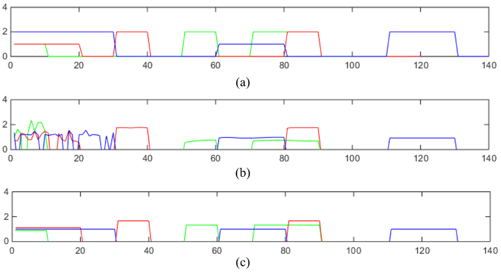
(a) represents the ground truth of u1, u2 and u3, where green represents u1, red represents u2, and blue represents u3. (b) Estimated u1, u2 and u3 by GSJNMF. (c) Estimated u1, u2 and u3 by GJNMFO.
We use the Pearson correlation coefficient to quantify the similarity between true ui and estimated ui by GSJNMF and GJNMFO (i = 1,2,3). As shown in Table III, the similarities between true ui and estimated ui by GSJNMF are 0.5713, 0.9073 and 0.7712, respectively. The similarities between true ui and estimated ui by GJNMFO are 0.9812, 0.9745 and 0.9370, respectively. From Table III, we can conclude that the performance of GJNMFO on similarity to the ground truth is better than that of GSJNMF. Furthermore, we use heat map drawing the correlation between any two columns in the basis matrix of GJNMFO and GSJNMF. As shown in Appendix B, the color of the heat map corresponding to GJNMFO is significantly cooler than GSJNMF, which shows that GJNMFO gets a higher incoherence between basis vectors. According to Ref. [25], high incoherence between basis vectors can guarantee that basis vectors are as discriminative as possible, which is the fundamental reason that the performance of GJNMFO is better than that of GSJNMF.
TABLE III.
The correlation coefficient between estimated ui and true ui (i = 1,2,3).
| methods | The correlation coefficient | ||
|---|---|---|---|
| correlation between u1 and | correlation between u2 and | correlation between u3 and | |
| GSJNMF | 0.5713 | 0.9073 | 0.7712 |
| GJNMFO | 0.9821 | 0.9745 | 0.9370 |
In order to make the dimension of simulated data closer to real one, we construct a new set of simulated data which dimension is 10 times the previous, i.e. , , and . The experimental results of GJNMFO and GSJNMF on this simulation data are illustrated in Appendix C, shown that GJNMFO is superior to GSJNMF even when the data is in a high dimension. Next, we use GJNMFO algorithm to analyze the risk genes, epigenetic factors and the abnormal brain ROIs of SZ.
3.4. Application on Schizophrenia Dataset
3.4.1. Real Data Preparation and Preprocessing
Schizophrenia is a complex mental disease in which people often characterized by brain abnormalities, genetic variations, and environmental factors[25]. It is very important to identify how genetics and environmental factors interact and affect brain function and cognition[26].
The SNP, DNA methylation and fMRI datasets used in this paper were collected by the Mind Clinical Imaging Consortium (MCIC) from 183 subjects, including 79 SZ patients (age: 34±11, 20 females) and 104 healthy controls (age: 32±11, 38 females). The fMRI data was collected while subjects were performing sensory motion task. Then, the data was pre-processed using SPM12 software and was realigned spatially normalized and resliced to 3 × 3 × 3 mm. It was smoothed with a 10 × 10 × 10 mm3 Gaussian kernel and analyzed by multiple regression considering the stimulus and their temporal derivatives plus an intercept term as repressors [27]. After these steps, the dimension of fMRI data is the 53*63*46. Then we select 41236 voxels from 116 brain regions according to the AAL brain atlas. The SNPs data was obtained from each subject’s blood sample. Genotyping for all participants was performed at the Mind Research Network, covering 1140419 SNP loci. Bead Studio was used to make the final genotype calls. PLINK software package (http://pngu.mgh.harvard.edu/~purcell/plink) was used to perform a series of standard quality control procedures, resulting in the final dataset spanning 777,635 SNP loci [9]. The DNA methylation data was obtained from the blood samples of the subjects, which assessed by the Illumina Infinium Methylation 27 k Assay. 27481 methylation CpG sites were selected after quality control[28], and 9273 methylation sites were further selected after removing sites with variance less than 1 × 10⁻⁴. Furthermore, we use the t-test to find biomarkers that are only associated with SZ, and only retain variables with P-value < 0.05. We obtain SNPs loci, fMRI voxels and DNA methylation CpG sites, respectively. Moreover, as shown in Fig. 6, we group SNPs loci, DNA methylation CpG sites, and fMRI voxels based on genes and ROIs (e.g., SNPs loci belong to the same gene, fMRI voxels belong to same ROI, DNA methylation CpG sites belong to the same gene). Then SNP, fMRI and DNA methylation datasets are divided into 3412, 72 and 1845 groups, respectively.
Fig. 6.
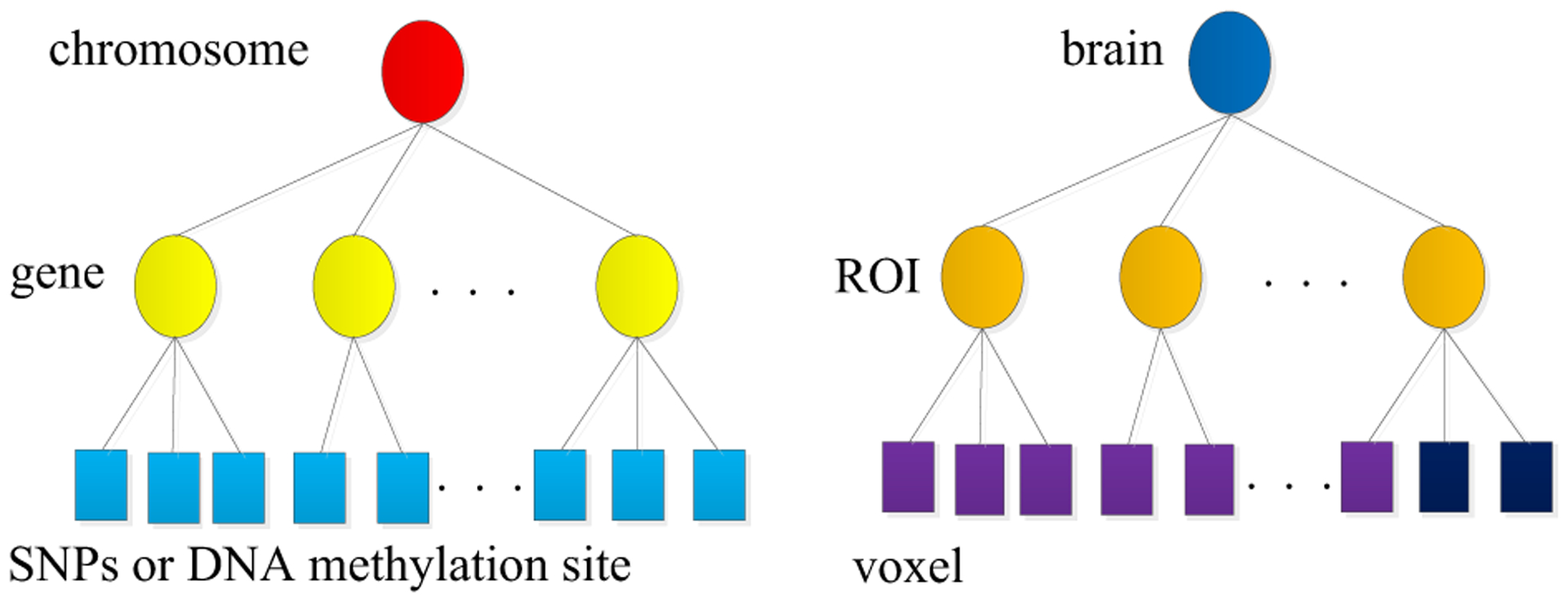
SNP loci, DNA methylation CpG sites and fMRI voxels can group by gene and ROI respectively.
3.4.2. Experimental Results on Real Data and Discussion
We apply GJNMFO algorithm to SNP, fMRI and DNA methylation datasets. In our experiment, the number of basis vector is set to 20 according to previous work [13]. We randomly initialize a set of non-negative W and Hi (i=1, 2, 3), and use the grid search method to determine the parameters of λ1, λ2 and λ3 within the range described above. In this way, a total of 1000 sets of parameters need to be brought into the model for calculation. Fig. 7 is the reconstruction error obtained by sequentially substituting 1000 sets of regularization parameters into algorithm 1. We use the set of regularization parameters corresponding to the minimum reconstruction error for further analysis.
Fig. 7.
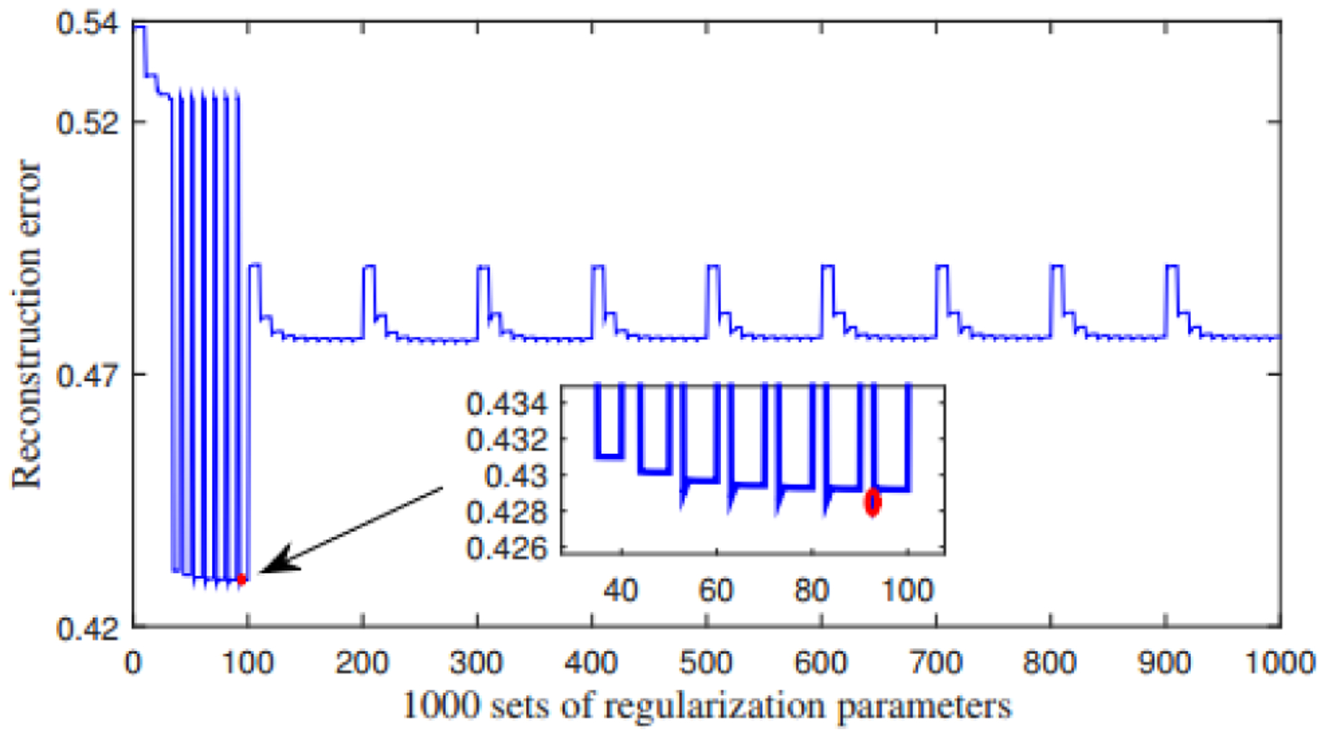
Reconstruction errors obtained under different combinations λ1, λ2 and λ3.
In Fig. 7, each point on the horizontal axis corresponds to a set of regularization parameters, and the vertical axis represents the reconstruction error obtained under the set of parameters. As can be seen from Fig. 7, when taking the 93rd group of regularization parameters, the reconstruction error is the smallest (i.e. the position of the red dot in Fig. 7). Parameters in group 93 are λ1=0.05, λ2=9.765×10⁻⁵ and λ3=0.0125.
We use this set of regularization parameters as the optimal one. To prevent the objective function Eq. (3) from falling into a local minimum, we repeat the whole procedure 100 times with different initialization values. When the objective function takes the minimum value, the corresponding W, H1, H2 and H3 are used for further analysis. We have drawn the values of the objective function under 100 sets of initialization value in Fig. 8.
Fig. 8.
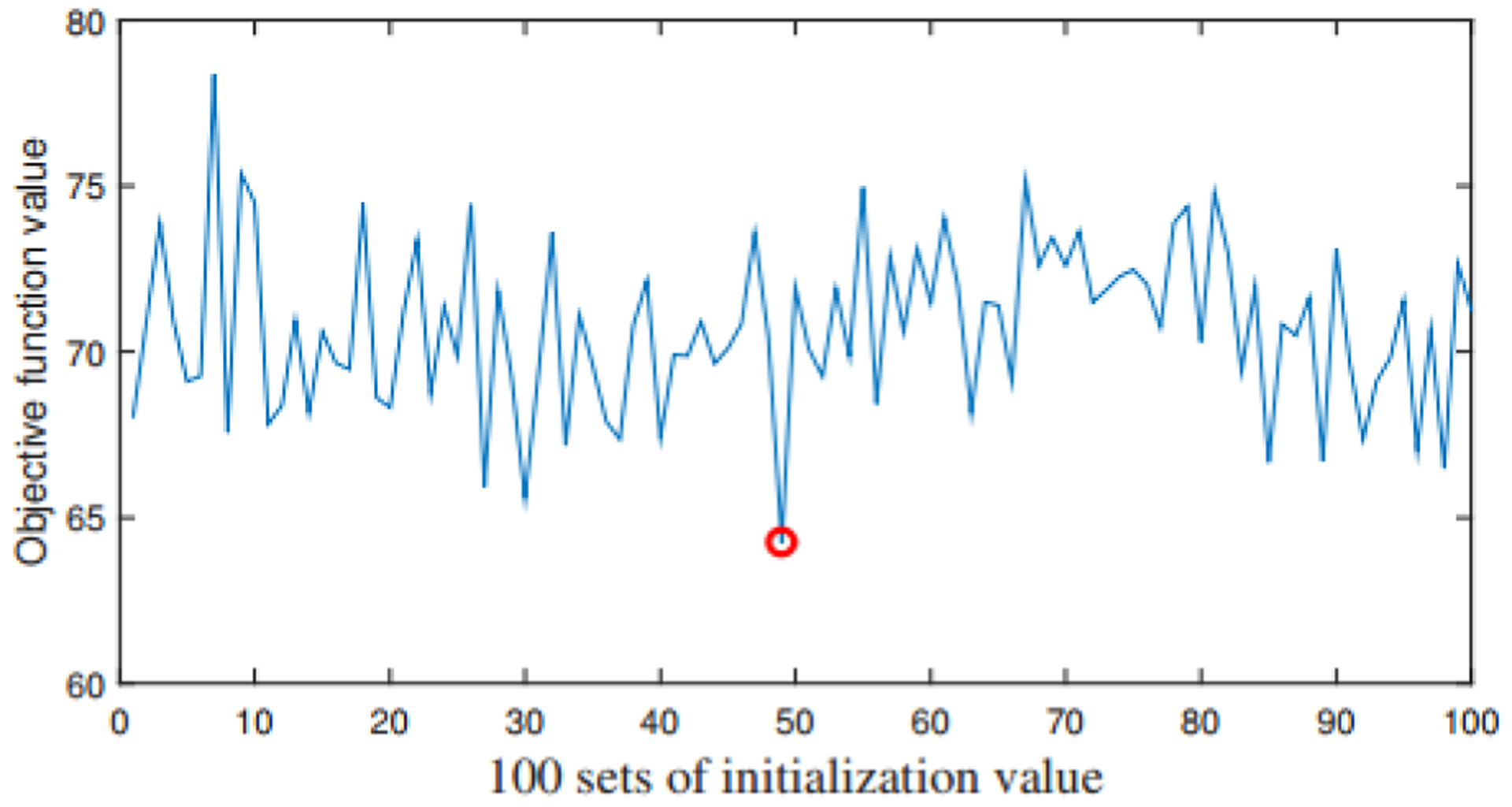
The value of objective function with different initialization value
We can see from the Fig. 8 that the 49-th initialization value corresponds to the smallest objective function value (i.e. the position of the red dot in Fig. 8), so we use W, H1, H2 and H3 obtained here to extract risk genes, epigenetic factors and abnormal ROIs. We calculate the z-score of H1, H2 and H3, and set T=3. If the element with z-score is less than T, then it is 0. In this way, we get a set of variables of each module, and then we use the above-mentioned significance test method (Eq. 16) to calculate the P-value of each module.
The modules with smallest P-value are further analyzed in this study. Table IV lists the genes identified by GJNMFO algorithm from the SNPs loci.
TABLE IV.
The List of the Gene Select from SNPs Data
| Module Index | Gene ID (SNP) |
|---|---|
| 19 | CNTN2 CDH4 ABCA4 AGBL4 ALDH9A1 C1orf161 C1orf163 CNTN2 DISC1 DNAH14 DNAJC11 DPYD ELAVL4 ELTD1 ESRRG FAM176A FAM46C FHL2 INSIG2FLJ35409 GPR177 HHAT KCNA3 KCND3 LMO4 KIRREL LOC100288925 LOC100289242 PLA2G4ALOC284661 LOC727944 LOC730134 LRRC38 OLFM3MYADML MYCN NPHP1 OTOF PADI4 PBX1 PLXNA2 PKP1 PRKCE QPCT RGS13 RNF144A RPS6KC1 RSBN1 SPATA1 ST6GALNAC3 TRIB2 TYW3 VAV3 VIT |
| 13 | KCNK9 ADORA3 AIM2 AJAP1 C1orf168 C2orf3NTNG1 CCDC85A CCDC88A CDC73 CYP2J2 FAM71A NGFFEZ2EZ2 FMO4 FMO9P GREM2 IL1R2 KIF26B LOC100129149 LOC126987 LOC644265 LOC728597 LOC730100 LRP8 LUZP1 MGST3 NT5C1B OLFML2B PDE4B PGBD5 RHOU SLC44A5 SRBD1 USP24 VPS13D |
As can be seen from Table IV, we identify a total of 54 risk genes from the SNPs data in the 19-th module. Since the protein encoded by CNTN2 has the function of adhering cells to help maintain the potassium ion channel in the correct position on the nerve fibers which plays an important role in the process of generating nerve impulses. Therefore, its mutation causes the nerve cells to behave abnormally. INSIG2 is associated with metabolic syndrome in patients with schizophrenia[29]. Lmo4 gene plays an important role in the development of the auditory nervous system[30]. OLFM3 is associated with a disorder of the metabolic pathway leading to low expression of nerve-specific genes, which causes neuronal weakness[31]. The abnormalities of PLA2G4A may be involved in a subgroup of the Schizophrenia. MaIl et al.[32] used genome-wide association studies to demonstrate that multiple sites in the PLXNA2 gene are significantly associated with SZ.
In the 13-th module, we identify a total of 36 risk genes from the SNPs data. KCNK9 is a key factor in the excitability of cortical neurons, which may cause defects in neuronal migration. NGF is associated with the onset and clinical symptoms of schizophrenia[33]. The NTNG1 gene is located in the lpl3.3 region of chromosome 1, and it is in a linked region with the onset of schizophrenia. In the family studies and case-control studies of the Japanese population, multiple SNPs loci of this gene have been found to be associated with schizophrenia[34]. PDE4B is an important enzyme in the nervous system, and recent studies have found it to play a decisive role in DISC1 mutation-induced schizophrenia[35].
To further illustrate the biological significance of the risk genes which list in table IV, we test genes for over-representation analysis using ConsensusPathDB[11, 36]. Table V lists the gene ontology terms that obtain by gene ontology categories with P-value less than 0.01 in biological process.
TABLE V.
The list of the gene ontology terms
| term name | p-value |
|---|---|
| neurogenesis | 0.00598 |
| neuron differentiation | 0.00477 |
| purinergic receptor signaling pathway | 0.00554 |
| G protein-coupled purinergic receptor signaling pathway | 0.0032 |
| icosanoid metabolic process | 0.00628 |
In table V, ‘neurogenesis’ and ‘neuron differentiation’ are related to the neural activity. ‘purinergic receptor signaling pathway’ has been confirmed to be related to neuronal differentiation, neuroprotection, and brain disorders[37]. G protein-coupled purinergic receptor is widely distributed in the nervous system and peripheral tissues, performing various physiological functions such as development and regeneration of the nervous system, regulating neurons, regulating memory function, regulating transmitter release, etc.[38]. Through the above analysis, we can conclude that the risk genes selected by GJNMFO from SNPs have biological significance. Table VI lists the epigenetic factors identified by GJNMFO algorithm from the DNA methylation dataset.
TABLE VI.
The List of the Gene Selected from DNA Methylation Data
| Module Index | Gene ID (DNA methylation) | |
|---|---|---|
| 19 | LOC201164 | RAET1L |
| 13 | C1orf26 | MTERF |
As shown in Table VI, 4 genes related to environmental factors are selected from DNA methylation dataset. ‘C10orf26’ also selected by Ref.[13], which is reported as one of the target of miR-137 to have genome-wide significant associations with SZ[39]. When mtDNA is transcribed to produce RNA, ‘MTERF’ is responsible for determining the location of mitochondrial transcription termination factors, Lauritzen et al.[40] demonstrated that point mutations in mitochondria may be associated with cognitive impairment of mental disease. Therefore, ‘MTERF’ is related to mental disease. Besides, ‘LOC201164’ is considered to be related to neural development in Ref.[41]. ‘RAET1L’ is an additional human NKG2D ligand which is related to the immune system[42], and clinical studies have shown that the immune system and brain function of patients with schizophrenia are abnormal. Table VII lists the brain ROIs selected by GJNMFO and adaptive SMCCA respectively.
TABLE VII.
Selected ROIs (fMRI) and Corresponding Areas
| GJNMFO | Adaptive SMCCA | ||
|---|---|---|---|
| ROI name | L/R volumn(cm3) | ROI name | L/R volumn(cm3) |
| Hippocampus | 1.59/* | Hippocampus | 1.65/* |
| Amygdala | 1.3/* | Frontal_Inf_Tri | 1.03/* |
| Occipital_Inf | */1.22 | Occipital_Inf | */1.22 |
| Fusiform_R | */0.678 | Fusiform | 1.86/1.00 |
| Temporal_Mid | */1.30 | ||
| Temporal_Inf | 2.11/* | ||
In table VII, GJNMFO algorithm selects a total of 4 ROIs and adaptive SMCCA selects a total of 6 ROIs. 3 ROIs are selected at the same time by GJNMFO and adaptive SMCCA algorithm. ‘Hippocampus gyrus’ is important in the consolidation of information from short-term memory to long-term memory, and is one of the first brain regions to suffer damage in mental disorders, and is also selected by Ref.[26] and Ref.[43]. The ‘occipital lobe’ is responsible for processing visual information. Occipital injury can make it difficult for schizophrenia patients to interpret complex images, recognize other people’s motives, and understand other people’s emotions. The volume of the ‘fusiform gyrus’ in patients with first-episode schizophrenia is reduced, and the reduction in the volume of the fusiform gyrus causes memory impairment [44]. ‘fusiform gyrus’ is selected by Ref.[13] and Ref.[26]. The volume of amygdala in patients with schizophrenia is 6% lower than that of normal subjects, and the decrease in amygdala volume is related to the recognition of facial emotions[45]. In order to illustrate the specific location of the abnormal brain region in brain surface, we use BrainNetViewer to plot the abnormal brain ROIs that selected by GJNMFO as shown in Fig. 9.
Fig. 9.
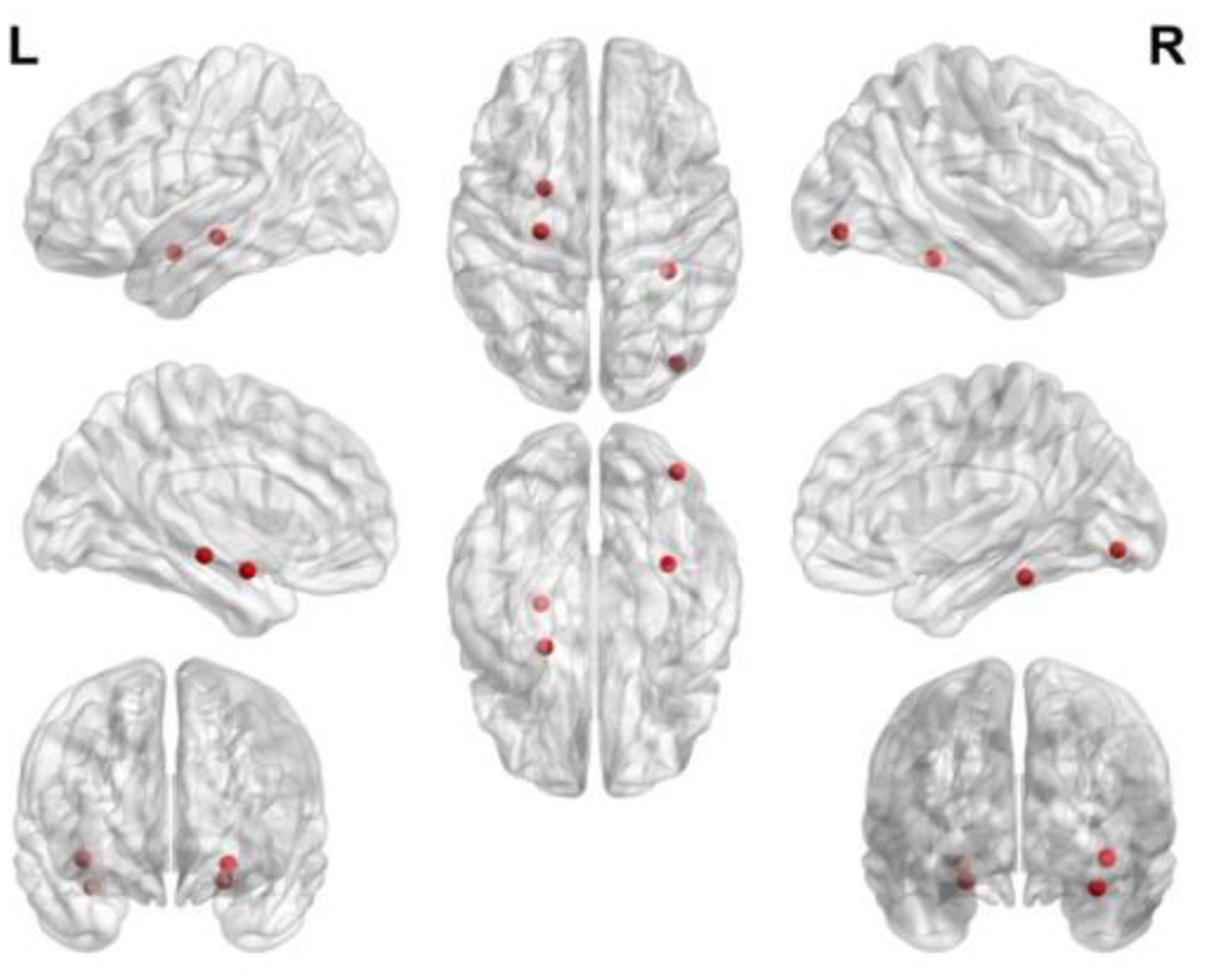
Abnormal ROIs selected by GJNMFO from fMRI data.
4. Conclusion
The main contributions of this paper can be summarized as follows. Firstly, we propose GJNMFO algorithm, which projects the multi-modal datasets of SZ into a new common low-dimensional space to identify risk genes, epigenetic factors and abnormal brain ROIs. The GJNMFO model integrates the orthogonal and group sparse constraint on the basis of the JNMF model. We employ orthogonal constraint to reduce the correlation between basis vectors, which helps remove insignificant features in the rows of coefficient matrix. In addition, since the imaging genetics datasets have rich group information, we employ group sparse constraint into the model as prior knowledge to make the extracted genetic variables and imaging variables more reasonable. Secondly, we describe the numerical optimization, significance estimation and parameters selection of GJNMFO algorithm. Thirdly, our algorithm is validated on simulation data and further applied on real data analysis. Simulation results show that our algorithm performs better than state-of-the-art algorithms GSJNMF and JNMF. Experimental results on real data indicate that our algorithm can identify more significant genes (PLA2G4A, INSIG2, etc.), epigenetic factors (C10orf26, MTERF, etc.) and abnormal ROIs (Hippocampus, Occipital_Inf, etc.), which are strong correlation with SZ and have been reported in many previous literatures. In conclusion, both simulation and real MCIC experiment results show that GJNMFO algorithm has outperformance in multi-modal imaging genetics data analysis.
Supplementary Material
Acknowledgment
This work was supported in part by the National Institutes of Health under Grant R01GM109068, Grant R01MH104680, Grant R01MH107354, RO1AR059781, R01EB006841, R01EB005846, and Grant P20GM103472, in part by the National Science Foundation (NSF), in part by the Fundamental Research Funds for the Central Universities, Chang’an University (CHD) NO. 300102329102, in part by the Natural Science Foundation of Shaanxi NO. 2019JM-536 and in part by the China Scholarship Council NO. 201806565009.
Contributor Information
Kaiming Wang, school of science, Chang’an University, Xi’an, Shaanxi, 710049, China..
Gang Li, school of Electronics and Control Engineering, Chang’an University, Xi’an, Shaanxi, 710049, China.
Vince D. Calhoun, The Mind Research Network, Albuquerque, NM, 87131, USA..
Yu-Ping Wang, Department of Biomedical Engineering, Tulane University, New Orleans, LA, 70118, USA..
References
- [1].Hariri AR, Drabant EM, and Weinberger DR, “Imaging genetics: perspectives from studies of genetically driven variation in serotonin function and corticolimbic affective processing,” Biological psychiatry, vol. 59, no. 10, pp. 888–897, 2006. [DOI] [PubMed] [Google Scholar]
- [2].Meyer-Lindenberg A, “The future of fMRI and genetics research,” NeuroImage, vol. 62, no. 2, pp. 1286–1292, 2012. [DOI] [PubMed] [Google Scholar]
- [3].Gottesman II and Gould TD, “The endophenotype concept in psychiatry: etymology and strategic intentions,” American Journal of Psychiatry, vol. 160, no. 4, pp. 636–645, 2003. [DOI] [PubMed] [Google Scholar]
- [4].Meyer-Lindenberg A and Weinberger DR, “Intermediate phenotypes and genetic mechanisms of psychiatric disorders,” Nature reviews neuroscience, vol. 7, no. 10, p. 818, 2006. [DOI] [PubMed] [Google Scholar]
- [5].Ge T, Schumann G, and Feng J, “Imaging genetics—towards discovery neuroscience,” Quantitative Biology, vol. 1, no. 4, pp. 227–245, 2013. [Google Scholar]
- [6].Hotelling H, “Relations between two sets of variates,” Biometrika, vol. 28, no. 3/4, pp. 321–377, 1936. [Google Scholar]
- [7].Parkhomenko E, Tritchler D, and Beyene J, “Sparse canonical correlation analysis with application to genomic data integration,” Statistical applications in genetics and molecular biology, vol. 8, no. 1, pp. 1–34, 2009. [DOI] [PubMed] [Google Scholar]
- [8].Witten DM, Tibshirani R, and Hastie T, “A penalized matrix decomposition, with applications to sparse principal components and canonical correlation analysis,” Biostatistics, vol. 10, no. 3, pp. 515–534, 2009. [DOI] [PMC free article] [PubMed] [Google Scholar]
- [9].Lin D, Calhoun VD, and Wang Y-P, “Correspondence between fMRI and SNP data by group sparse canonical correlation analysis,” Medical image analysis, vol. 18, no. 6, pp. 891–902, 2014. [DOI] [PMC free article] [PubMed] [Google Scholar]
- [10].Du L et al. , “Structured sparse canonical correlation analysis for brain imaging genetics: an improved GraphNet method,” Bioinformatics Medical image analysis, vol. 32, no. 10, pp. 1544–1551, 2016. [DOI] [PMC free article] [PubMed] [Google Scholar]
- [11].Hu W et al. , “Adaptive sparse multiple canonical correlation analysis with application to imaging (epi) genomics study of schizophrenia,” IEEE Transactions on Biomedical Engineering, vol. 65, no. 2, pp. 390–399, 2018. [DOI] [PMC free article] [PubMed] [Google Scholar]
- [12].Lee DD and Seung HS, “Learning the parts of objects by non-negative matrix factorization,” Nature Australia, vol. 401, no. 6755, p. 788, 1999. [DOI] [PubMed] [Google Scholar]
- [13].Wang M, Huang T-Z, Fang J, Calhoun VD, and Wang Y-P, “Integration of imaging (epi) genomics data for the study of schizophrenia using group sparse joint nonnegative matrix factorization,” IEEE/ACM transactions on computational biology and bioinformatics, 2019. [DOI] [PMC free article] [PubMed] [Google Scholar]
- [14].Kim J, Monteiro RD, and Park H, “Group sparsity in nonnegative matrix factorization,” in Proceedings of the SIAM International Conference on Data Mining, 2012, pp. 851–862: SIAM. [Google Scholar]
- [15].Yuan M and Lin Y, “Model selection and estimation in regression with grouped variables,” Journal of the Royal Statistical Society: Series B (Statistical Methodology), vol. 68, no. 1, pp. 49–67, 2006. [Google Scholar]
- [16].Zhang S, Liu C-C, Li W, Shen H, Laird PW, and Zhou XJ, “Discovery of multi-dimensional modules by integrative analysis of cancer genomic data,” Nucleic acids research, vol. 40, no. 19, pp. 9379–9391, 2012. [DOI] [PMC free article] [PubMed] [Google Scholar]
- [17].Liu W and Zheng N, “Non-negative matrix factorization based methods for object recognition,” Pattern Recognition Letters, vol. 25, no. 8, pp. 893–897, 2004. [Google Scholar]
- [18].Shahnaz F, Berry MW, Pauca VP, and Plemmons RJ, “Document clustering using nonnegative matrix factorization,” Information ProcessingManagement data series. Parks and Wildlife Department (Texas), vol. 42, no. 2, pp. 373–386, 2006. [Google Scholar]
- [19].Berry MW, Browne M, Langville AN, Pauca VP, and Plemmons RJ, “Algorithms and applications for approximate nonnegative matrix factorization,” Computational Statistics & Data Analysis, vol. 52, no. 1, pp. 155–173, 2007. [Google Scholar]
- [20].Xu Y and Qian Y, “Group sparse nonnegative matrix factorization for hyperspectral image denoising,” in Geoscience & Remote Sensing Symposium, 2016. [Google Scholar]
- [21].Li Z, Wu X, and Peng H, “Nonnegative matrix factorization on orthogonal subspace,” Pattern Recognition Letters, vol. 31, no. 9, pp. 905–911, 2010. [Google Scholar]
- [22].Kuhn HW, “Nonlinear programming: a historical view,” ACM SIGMAP Bulletin, no. 31, pp. 6–18, 1982. [Google Scholar]
- [23].Brunet J-P, Tamayo P, Golub TR, and Mesirov JP, “Metagenes and molecular pattern discovery using matrix factorization,” Proceedings of the national academy of sciences, vol. 101, no. 12, pp. 4164–4169, 2004. [DOI] [PMC free article] [PubMed] [Google Scholar]
- [24].Chen X, Han L, and Carbonell J, “Structured sparse canonical correlation analysis,” in Artificial Intelligence and Statistics, pp. 199–207, 2012 [Google Scholar]
- [25].Fang J, Lin D, Schulz SC, Xu Z, Calhoun VD, and Wang Y-P, “Joint sparse canonical correlation analysis for detecting differential imaging genetics modules,” Bioinformatics Medical image analysis, vol. 32, no. 22, pp. 3480–3488, 2016. [DOI] [PMC free article] [PubMed] [Google Scholar]
- [26].Hu W, Lin D, Calhoun VD, and Wang Y.-p., “Integration of SNPs-FMRI-methylation data with sparse multi-CCA for schizophrenia study,” in Medicine and Biology Society (EMBC), IEEE 38th Annual International Conference of the Engineering, 2016, pp. 3310–3313: IEEE. [DOI] [PubMed] [Google Scholar]
- [27].Landeau B, “Automated anatomical labeling of activations in SPM using a macroscopic anatomical parcellation of the MNI MRI single-subject brain,” Neuroimage, vol. 15, no. 1, pp. 273–289, 2002. [DOI] [PubMed] [Google Scholar]
- [28].Jingyu L et al. , “Methylation patterns in whole blood correlate with symptoms in schizophrenia patients,” Schizophrenia Bulletin, vol. 40, no. 4, p. 769, 2014. [DOI] [PMC free article] [PubMed] [Google Scholar]
- [29].Liou YJ et al. , “Gene–gene interactions of the INSIG1 and INSIG2 in metabolic syndrome in schizophrenic patients treated with atypical antipsychotics,” Pharmacogenomics Journal, vol. 12, no. 1, p. 54, 2012. [DOI] [PubMed] [Google Scholar]
- [30].Min D et al. , “LMO4 functions as a negative regulator of sensory organ formation in the mammalian cochlea,” Journal of Neuroscience, vol. 34, no. 30, pp. 10072–10077, 2014. [DOI] [PMC free article] [PubMed] [Google Scholar]
- [31].Vita A, De PL, Deste G, and Sacchetti E, “Progressive loss of cortical gray matter in schizophrenia: a meta-analysis and meta-regression of longitudinal MRI studies,” Translational Psychiatry, vol. 2, no. 11, p. e190, 2012. [DOI] [PMC free article] [PubMed] [Google Scholar]
- [32].Mah S et al. , “Identification of the semaphorin receptor PLXNA2 as a candidate for susceptibility to schizophrenia,” Molecular Psychiatry, vol. 11, no. 5, pp. 471–478, 2006. [DOI] [PubMed] [Google Scholar]
- [33].Martinotti G, Di IG, Marini S, Ricci V, De BD, and Di GM, “Nerve growth factor and brain-derived neurotrophic factor concentrations in schizophrenia: a review,” Journal of Biological Regulators & Homeostatic Agents, vol. 26, no. 3, p. 347, 2012. [PubMed] [Google Scholar]
- [34].Ohtsuki T et al. , “Association of polymorphisms in the haplotype block spanning the alternatively spliced exons of the NTNG1 gene at 1p13.3 with schizophrenia in Japanese populations,” Neuroscience Letters, vol. 435, no. 3, pp. 194–197, 2008. [DOI] [PubMed] [Google Scholar]
- [35].J Kirsty M et al. , “DISC1 and PDE4B are interacting genetic factors in schizophrenia that regulate cAMP signaling,” Science, vol. 310, no. 5751, pp. 1187–1191, 2005. [DOI] [PubMed] [Google Scholar]
- [36].Kamburov A, Stelzl U, Lehrach H, and Herwig R, “The ConsensusPathDB interaction database: 2013 update,” Nucleic acids research, vol. 41, no. D1, pp. D793–D800, 2013. [DOI] [PMC free article] [PubMed] [Google Scholar]
- [37].Majumder P et al. , “New insights into purinergic receptor signaling in neuronal differentiation, neuroprotection, and brain disorders,” Purinergic Signalling, vol. 3, no. 4, pp. 317–331, 2007. [DOI] [PMC free article] [PubMed] [Google Scholar]
- [38].Illes P, Verkhratsky A, Burnstock G, and Franke H, “P2X receptors and their roles in astroglia in the central and peripheral nervous system,” Neuroscientist, vol. 18, no. 5, pp. 422–438, 2012. [DOI] [PubMed] [Google Scholar]
- [39].Kwon E, Wang W, and Tsai L-H, “Validation of schizophrenia-associated genes CSMD1, C10orf26, CACNA1C and TCF4 as miR-137 targets,” Mol Psychiatry, vol. 18, no. 1, pp. 11–12, 2013. [DOI] [PubMed] [Google Scholar]
- [40].Lauritzen KH et al. , “Mitochondrial DNA toxicity in forebrain neurons causes apoptosis, neurodegeneration, and impaired behavior,” Molecular and cellular biology, vol. 30, no. 6, pp. 1357–1367, 2010. [DOI] [PMC free article] [PubMed] [Google Scholar]
- [41].Kerkel K et al. , “Altered DNA Methylation in Leukocytes with Trisomy 21,” Plos Genetics, vol. 6, no. 11, p. e1001212, 2010. [DOI] [PMC free article] [PubMed] [Google Scholar]
- [42].Eagle RA, Traherne JA, Hair JR, Jafferji I, and Trowsdale J, “ULBP6/RAET1L is an additional human NKG2D ligand,” European Journal of Immunology, vol. 39, no. 11, pp. 3207–3216, 2010. [DOI] [PubMed] [Google Scholar]
- [43].Ozdemir H, Ertugrul A, Basar K, and Saka E, “Differential effects of antipsychotics on hippocampal presynaptic protein expressions and recognition memory in a schizophrenia model in mice,” Progress in Neuro-Psychopharmacology and Biological Psychiatry, vol. 39, no. 1, pp. 62–68, 2012. [DOI] [PubMed] [Google Scholar]
- [44].Uk LC et al. , “Fusiform gyrus volume reduction in first-episode schizophrenia: a magnetic resonance imaging study,” Archives of General Psychiatry, vol. 59, no. 9, p. 775, 2002. [DOI] [PubMed] [Google Scholar]
- [45].Namiki C et al. , “Impaired facial emotion recognition and reduced amygdalar volume in schizophrenia,” Psychiatry Res, vol. 156, no. 1, pp. 23–32, 2007. [DOI] [PubMed] [Google Scholar]
Associated Data
This section collects any data citations, data availability statements, or supplementary materials included in this article.


