

Abstract
Background
Stroke is a major cardiovascular disease that causes significant health and economic burden in the United States. Neighborhood community‐based interventions have been shown to be both effective and cost‐effective in preventing cardiovascular disease. There is a dearth of robust studies identifying the key determinants of cardiovascular disease and the underlying effect mechanisms at the neighborhood level. We aim to contribute to the evidence base for neighborhood cardiovascular health research.
Methods and Results
We created a new neighborhood health data set at the census tract level by integrating 4 types of potential predictors, including unhealthy behaviors, prevention measures, sociodemographic factors, and environmental measures from multiple data sources. We used 4 tree‐based machine learning techniques to identify the most critical neighborhood‐level factors in predicting the neighborhood‐level prevalence of stroke, and compared their predictive performance for variable selection. We further quantified the effects of the identified determinants on stroke prevalence using a Bayesian linear regression model. Of the 5 most important predictors identified by our method, higher prevalence of low physical activity, larger share of older adults, higher percentage of non‐Hispanic Black people, and higher ozone levels were associated with higher prevalence of stroke at the neighborhood level. Higher median household income was linked to lower prevalence. The most important interaction term showed an exacerbated adverse effect of aging and low physical activity on the neighborhood‐level prevalence of stroke.
Conclusions
Tree‐based machine learning provides insights into underlying drivers of neighborhood cardiovascular health by discovering the most important determinants from a wide range of factors in an agnostic, data‐driven, and reproducible way. The identified major determinants and the interactive mechanism can be used to prioritize and allocate resources to optimize community‐level interventions for stroke prevention.
Keywords: cardiovascular health, neighborhood, prevention, tree‐based machine learning, variable selection
Subject Categories: Risk Factors, Cerebrovascular Disease/Stroke, Health Services
Nonstandard Abbreviations and Acronyms
- BART
Bayesian additive regression trees
- gbm
gradient boosting machines
- LR
linear regression
- OOB
out‐of-bag
- RF
random forests
- RMSE
root mean squared error
- VIPs
variable inclusion proportions
- XGBoost
extreme gradient boosting
Clinical Perspective
What Is New?
A new large‐scale neighborhood health data set at the census tract level was created from multiple sources; principled variable selection algorithms exploiting tree‐based machine learning techniques were used to identify key neighborhood‐level predictors for the neighborhood‐level prevalence of stroke.
Our approach identified a parsimonious set of most important predictors without much loss of prediction accuracy.
Higher prevalence of low physical activity, larger share of older adults, higher percentage of non‐Hispanic Black people, and higher ozone levels were associated with higher prevalence of stroke at the neighborhood level; higher median household income was linked to lower prevalence.
What Are the Clinical Implications?
The identified major determinants can help prioritize and allocate resources for community‐level stroke interventions.
Stroke is a major chronic disease costing the US healthcare system billions of dollars a year. 1 Identifying modifiable risk factors for stroke is important for developing effective prevention strategies. Existing epidemiological studies on stroke primarily focused on individual‐level risk factors, such as demographic factors (eg, age, race/ethnicity), socioeconomic factors (eg, income, education), and health behaviors (eg, diet, physical activity). 2 , 3 , 4 , 5 Air pollution exposures have also been shown to adversely affect the cardiovascular system and increase stroke‐related healthcare use. 2 , 6 These individual‐level factors have been incorporated into intervention programs to prevent and control stroke. 7 , 8 , 9
In addition to individual‐based interventions, targeted neighborhood‐level interventions have been shown to be more cost‐effective in preventing stroke. 10 However, little attention has been paid to neighborhood‐level factors that may be associated with stroke, despite the fact that growing evidence supports that the condition of a neighborhood significantly affects the inhabitants' health. 11 , 12 Consequently, there is a lack of understanding of the underlying mechanisms between neighborhood characteristics and the prevalence of stroke at the neighborhood level.
To fill these research gaps, this study aims to identify a crucial set of risk factors that have important effects on the neighborhood‐level prevalence of stroke with methodological rigor. We implemented several state‐of‐the‐art tree‐based machine learning techniques on new neighborhood‐level health data combining information from multiple sources. We modeled the relationship between neighborhood‐level predictors and the neighborhood‐level prevalence of stroke, treating each census tract as the unit of analysis. We considered 24 factors that have been linked to cardiovascular health outcomes at the individual patient level from 4 major domains, unhealthy behaviors, prevention measures, sociodemographic indicators, and environmental measures. 3 , 4 , 5 , 13 We then used principled variable selection algorithms based on our machine learning model outputs to identify most important predictors and compared the relative importance of selected predictors in an agonistic way. We further compared the predictive performance of the tree‐based methods considered and demonstrated their operating characteristics for variable selection. Finally, we quantified how the identified major predictors may have influenced the prevalence of stroke at the neighborhood level. Results from this study will provide insights into developing tailored community‐based stroke‐prevention strategies.
Methods
Data Source
We generated a large neighborhood health data by integrating public domain information at the census tract level from the Centers for Disease Control and Prevention, the Census Bureau, and the Environmental Protection Agency in the United States. We used census tract as a proxy of neighborhood. The first data set included the prevalence of health outcomes, prevention, and health behavior measures from the Centers for Disease Control and Prevention's 500 Cities Data for 28 004 census tracts. 14 This data set is publicly available on its website, https://chronicdata.cdc.gov/browse?category=500+Cities. The second data set focused on sociodemographic measures using the 2011–2015 American Community Survey, 15 , 16 publicly available at https://www.census.gov/data/developers/data-sets/acs-5year.html. We also included environmental exposure data from the Environmental Protection Agency's 2015–2016 Environmental Justice Screening database, 17 publicly available at https://www.epa.gov/ejscreen/download-ejscreen-data. This study used publicly available ecological data and is not considered a human subject study; therefore, the study was exempted from obtaining approval of the institutional review board for ethics committee and individual informed consent. The analysis codes that support the findings of this study are available from the corresponding author upon reasonable request.
We included 24 potential predictors from 4 domains: (1) unhealthy behaviors (eg, no leisure‐time physical activity, obesity), (2) prevention measures (eg, lack of health insurance), (3) sociodemographic indicators (eg, race/ethnicity, income level), and (4) environmental measures (eg, ambient air pollution). Both stroke and predictors were measured at the neighborhood level (no person‐level data were used). Table 1 details all 24 variables, their data sources and their descriptive distributions. We excluded 1307 census tracts with no information on key variables. Among the 1307 census tracts, 137 had missing data on sociodemographic variables, 875 did not have health measures, and 295 had no environmental information. Our final analysis data set included 26 697 census tracts.
Table 1.
Distribution of 24 Potential Neighborhood‐Level Predictors and Prevalence of Stroke Across 26 697 Census Tracts in 500 Major US Cities
| Domain | Variable Name | Definition | (Min, Max) | Median (Q1–Q3) | Mean (SD) | Data Source |
|---|---|---|---|---|---|---|
| Health outcomes | STROKE | Stroke among adults aged ≥18 y | (0.30, 18.80) | 2.80 (2.20–3.60) | 3.11 (1.43) | CDC 500 Cities Data |
| Unhealthy behaviors | SMOKING | Current smoking among adults aged ≥18 y | (2.00, 48.70) | 18.30 (14.30–23.10) | 19.10 (6.42) | CDC 500 Cities Data* |
| NO_PA | No leisure‐time physical activity among adults aged ≥18 y | (7.90, 61.30) | 24.20 (18.30–31.60) | 25.30 (8.62) | ||
| OBESITY | Obesity among adults aged ≥18 y | (8.70, 58.50) | 28.60 (23.70–34.90) | 29.76 (8.06) | ||
| INSUF_SLEEP | Sleeping <7 h among adults aged ≥18 y | (18.50, 59.80) | 36.30 (32.50–41.20) | 37.10 (6.42) | ||
| Prevention | LACK_INSURANCE | Current lack of health insurance among adults aged 18–64 y | (2.50, 70.80) | 18.00 (11.70–27.40) | 20.58 (11.27) | CDC 500 Cities Data |
| DENTAL | Visits to dentist or dental clinic among adults aged ≥18 y | (18.90, 87.10) | 61.30 (49.80–70.50) | 59.82 (13.16) | ||
| COLON_SCREEN | Fecal occult blood test, sigmoidoscopy, or colonoscopy among adults aged 50–75 y | (23.40, 81.50) | 60.60 (52.60–66.60) | 59.29 (9.38) | ||
| CORE_PREV_M | Older adults aged ≥65 y who are up to date on a core set of clinical preventive services (men: flu shot past year, pneumococcal polysaccharides vaccine [PPV] shot ever, colorectal cancer screening) | (13.10, 52.20) | 29.90 (24.80–34.60) | 29.88 (6.50) | ||
| CORE_PREV_W | Older adults aged ≥65 y who are up to date on a core set of clinical preventive services (women: same as above and mammogram past 2 y) | (9.60, 53.80) | 28.60 (23.00–33.90) | 28.64 (7.32) | ||
| Sociodemographic status | AGE65_OVER | Population aged ≥65 | (0.00, 100.00) | 14.81 (10.61–19.79) | 15.81 (8.02) | ACS† |
| AGE18_34 | Population aged between 18 and 34 | (0.00, 100.00) | 33.68 (27.28–40.74) | 35.01 (12.63) | ||
| COLLEGE_HIGHER | Bachelor's degree or higher | (0.00, 100.00) | 23.71 (12.27–40.33) | 28.28 (19.62) | ||
| HS_COLLEGE | High school graduate or higher | (0.00, 100.00) | 85.51 (75.78–91.66) | 82.44 (11.87) | ||
| FEMALE | Female | (0.00, 100.00) | 51.19 (48.82–53.60) | 51.04 (4.99) | ||
| NON_HIS_ASIAN | Not Hispanic or Latino—Asian alone | (0.00, 91.32) | 3.08 (0.72–8.50) | 7.26 (11.36) | ||
| NON_HIS_BLACK | Not Hispanic or Latino—Black or African American alone | (0.00, 100.00) | 7.37 (2.19–24.43) | 19.73 (26.69) | ||
| NON_HIS_OTHER | Not Hispanic or Latino—Other | (0.00, 119.45) | 4.61 (2.07–8.06) | 6.02 (6.44) | ||
| NON_HIS_WHITE | Not Hispanic or Latino—White alone | (0.00, 100.00) | 48.02 (17.24–72.15) | 45.65 (29.55) | ||
| POVERTY | Below poverty level; estimate; families | (0.00, 100.00) | 12.10 (5.1 0–24.00) | 16.09 (13.91) | ||
| MED_INCOME‡ | Median household income in the past 12 mo (in thousands) | (4.17, 250.00) | 49.58 (34.10–70.43) | 55.49 (29.17) | ||
| Environmental factors | HOUSE_PRE1960‡ | Pre‐1960 housing (lead paint indicator) (in thousands) | (0.00, 8.13) | 0.48 (0.10–0.92) | 0.59 (0.56) | |
| TRAFFIC‡ | Traffic proximity and volume (average number of vehicles/distance) | (0.00, 62.11) | 0.39 (0.12–1.10) | 1.17 (2.75) | ||
| OZONE‡ | Ozone level in air (ppb) | (27.63, 73.67) | 48.74 (44.40–52.81) | 48.04 (8.13) | EPA‐EJSCREEN§ | |
| PM25‡ |
PM2.5 level in air (μg/m3) |
(4.97, 13.32) | 9.89 (8.54–10.66) | 9.71 (1.53) |
Measures are in percentages for all variables except those marked with a double dagger. PM indicates particulate matter; Q1 indicates first quantile; and Q3, third quantile.
Census tract level 500 Cities Data from the Centers for Disease Control and Prevention (CDC), which were modeled based on population‐based survey data from the Behavioral Risk Factor Surveillance System.
Census tract level data from the 2011–2015 American Community Survey 5‐Year Estimates provided by the Census Bureau.
Indicates variables with absolute measurements as opposed to percentages.
To match the geospatial unit of census tract available in the other 2 data sources, we aggregated the census block group level environmental measures to the census tract level by taking the means for PM2.5 and O3, and the sum for the housing data, and the sum of block‐group‐level population weighted traffic proximity data. PM2.5 concentrations are annual average of the daily ambient average, and ozone concentrations are average of daily maximum 8‐hour level for the summer season. Both PM2.5 and ozone were from a space‐time downscaling fusion model based on monitoring data and modeled data. Traffic data reflect annual average daily traffic count of vehicles, that is, count of vehicle at major roads within 500 meters divided by distance in meters, and was calculated based on traffic data from the US Department of Transportation. Pre‐1960 housing data were based on the American Community Survey from the US Census.
Tree‐Based Machine Learning Methods
We considered 4 tree‐based machine learning methods, Bayesian additive regression trees (BART), 18 gradient boosting machines (gbm), 19 extreme gradient boosting (XGBoost) 20 and random forests (RFs). 21 We compared their performance in predicting the neighborhood‐level prevalence of stroke, implemented variable selection using each of the 4 methods, and provided insights into the key determinants selected by each method. We briefly introduce each method considered.
Bayesian Additive Regression Trees
BART is a nonparametric Bayesian approach using regression trees. A regression tree T approximates the covariate‐outcome relationship by recursive binary partitioning of the predictor space based on the importance of each predictor to the outcome. The tree T consists of the tree structure and all the decision rules sending a variable either left or right and leading down to a bottom node. Each of the bottom nodes represents the mean response of the subgroup of observations that fall in that node. The tree T can then be used as a prediction model. Tree‐based regression models are adept at fitting interactions and nonlinearities. An ensemble of regression trees have heightened modeling flexibility and better prediction accuracy. 22 BART is a “sum‐of‐trees” ensemble, relying on a fully Bayesian probabilistic model. A regularization prior is placed to 3 components of each tree—the tree structure itself, the tree parameters given the tree structure, and the error variance—so that each tree is constrained to contribute only a small part to the “sum‐of‐trees” model, which is remarkably stable and avoids overfitting. An iterative Bayesian back‐fitting Markov chain Monte Carlo algorithm generates samples from the posterior of each of the 3 components, which can then be used for prediction. Recently, BART has gained popularity in the statistical machine learning community for its superior predictive performance against several competing machine learning methods, including RFs, boosted models, and neural nets, in a variety of study settings. 18 , 23 , 24
Boosting (gbm and XGBoost)
Boosting is an ensemble approach to improve the predictive performance of a single regression tree T. 19 , 25 Boosting grows the trees slowly and sequentially each time taking into account information from previously constructed trees. In this process, boosting boosts a weak learner into a strong learner. Friedman et al 25 connected boosting to a forward stagewise additive model that minimizes a loss function. This new statistical perspective brought forth a highly adaptable algorithm, gradient boosting machines. Friedman further incorporated the bagging technique 21 to form “stochastic gradient boosting.” The key steps of a gradient boosting algorithm are as follows: (1) Initialize the algorithm with the best guess of the response, for example, observed response proportion; (2) compute the residual, or gradient, and fit a tree model to the residuals to minimize the exponential loss; (3) add the current tree model to the previous one; and (4) iterate steps (2) and (3) for a prespecified number of times. This technique is commonly referred to as gbm. Boosting has 3 tuning parameters, the number of trees, the shrinkage parameter, and the number of splits in each tree. XGBoost is further developed to optimize the boosting trees algorithms. 20 The underlying algorithm of XGBoost extends the classic gbm algorithm. By employing multithreads and imposing regularization, XGBoost is able to use more computational power and generate more accurate prediction.
Random Forests
The RF model is another ensemble technique to improve the predictive accuracy of a single regression tree T. The key ideas of the RF approach are bagging—short for bootstrap aggregation—and randomly selecting a smaller set of predictors to be considered for each split. 21 Bagging uses bootstrapping together with the single decision tree algorithm to build an ensemble. Because of the bootstrap resampling technique, bagging supplies out‐of‐bag (OOB) error for measuring predictive accuracy of the bagged model. At each iteration of bootstrapping, certain samples are left out and not used for fitting the tree model in that iteration. These samples are called OOB samples and can be used to evaluate the predictive performance of the tree model in that iteration. In this way, we can record B performance measures from the B bootstrapped samples. Averaging the B measures over the entire ensemble yields the OOB error. Bagging generates a distribution of trees that may share common structures, which induces tree correlations and consequently prohibits a bagged model from ideally reducing variance of predicted outcomes. To reduce correlation among bootstrapped trees and consequently improve the predictive performance of the ensemble, the RF technique considers a random subset of predictors for each split in the tree‐building process on each bootstrap sample. A typical RF's tuning parameters are the number of randomly selected predictors and the number of trees.
Variable Selection Using Tree‐Based Methods
BART‐Machine
We implemented a variable selection procedure, BART‐Machine, developed in Bleich et al 26 to uncover a parsimonious set of most critical predictors for the prevalence of stroke at the neighborhood level. This method performs favorably compared with variable selection using importance scores of RF. BART‐Machine uses the variable inclusion proportions (VIPs), that is, the proportion of times each variable is selected as a splitting rule divided by the total number of splitting rules in building the model, as the measure of variable importance, and then compares the VIPs on the basis of the observed data to the distributions of VIPs computed from 100 permutated data sets to decide whether a variable has a large enough VIP and should be regarded as important. This procedure identifies variables that have real important effects on the response rather than appear to be important by chance alone. We described the BART‐Machine algorithm in Figure 1.
Figure 1. Variable selection algorithm using BART‐Machine.
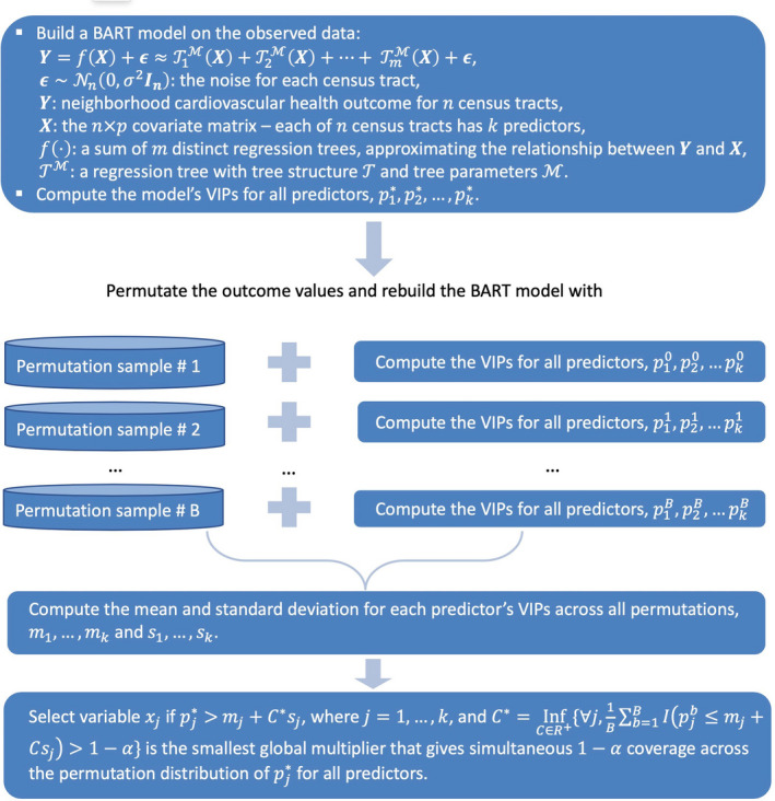
BART indicates Bayesian Additive Regression Trees; and VIP, variable inclusion proportions.
Following the selection of major predictors, we examined interaction effects with a BART model. Variables were considered to interact in a tree only if they appeared together in a contiguous downward path from the top to the bottom of the tree. We computed the total number of interactions for each pair of predictors by summing across trees and Markov chain Monte Carlo iterations, from which relative importance of each interaction was evaluated.
Boosting and RFs
Both boosting (gbm and XGBoost) and RFs provide the variable importance scores. For RFs, we measured the importance magnitude of a predictor by recording the improvement in the Gini index each time the predictor in a nonterminal node is selected for splitting. Then these individual improvement records for each predictor were averaged over the OOB samples of all the trees in the forest to quantify the overall relative importance of the predictors. For boosting, the important scores were calculated in a similar fashion and were scaled and referred to as relative influence scores. We used the variable importance score supplied by the RF algorithm and implemented an iterative procedure described in Jiang et al. 27 Dietrich et al. 28 and Hu et al. 29 for variable selection. Briefly, (1) compute an RF or boosting model using all of the 24 candidate predictors; (2) rank the predictors by variable importance and remove the predictor with the least importance score from the data; (3) compute a new RF or boosting model with the remaining data; (4) repeat steps (2) and (3) until only 1 predictor remains; and (5) choose the set of predictors with the smallest prediction error rate (OOB error for RF, cross‐validation error for gbm and XGBoost).
Assessing Advantages of Machine Learning for Variable Selection
We first compared the predictive performance of the 4 tree‐based methods using repeated 5‐fold cross validation on the basis of root mean squared error (RMSE). 30 We then applied these machine learning methods for variable selection and further compared them with 2 alternative methods frequently used in public health research: main effects linear regression (LR) including all predictors, termed as LR‐AllVar, and stepwise LR variable selection, referred to as LR‐StepWise. 31 , 32 LR‐StepWise starts with all predictors in the model and removed predictors based on P values until all remaining variables are statistically significant in the model; the best final model is chosen with the smallest Akaike Information Criterion. For a fair comparison of the methods based only on their capability to identify most important predictors, we included variables (both individual variables and interaction terms) selected by tree‐based methods in a LR model, and computed RMSE and RMSE reduction per predictor for each method. Thus, the difference in the performance metrics will be attributable to only the selected variables and not confounded by the predictive performance of different models. RMSE reduction per predictor is defined as (RMSEnull−RMSEmethod)/Number of Predictorsmethod, where RMSEnull is the RMSE from the null model (ie, intercept only model), and RMSEmethod corresponds to the RMSE of each specific method. This performance metric answers the question of how much gain do we get for adding each predictor variable suggested by a variable selection approach. Methods that give larger RMSE reduction per predictor variable are preferred. 26
Finally, to increase the interpretability, we quantified the associations between the identified major predictors and interaction terms and stroke prevalence using a Bayesian linear regression model. 33 All statistical analysis were performed using the R software version 3.6.1.
Results
Comparison of Predictive Performance of Tree‐Based Methods
We used repeated cross validation with 5 folds and 200 replications to compare the prediction accuracy of the 5 tree‐based method considered. Figure 2 displays boxplots of the cross‐validated RMSEs for the 4 tree‐based methods. BART appeared to be the top performer with the lowest RMSE, followed by XGBoost. The RFs had the largest RMSE.
Figure 2. Comparison of Cross‐validated (CV) root mean squared error (RMSE) for each of 4 tree‐based methods.
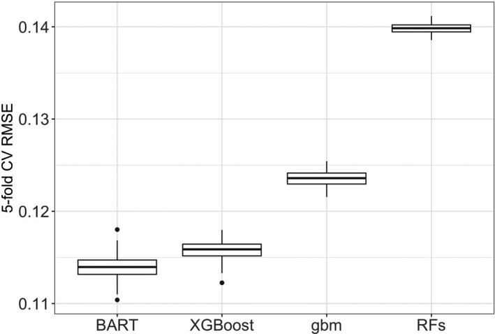
BART indicates Bayesian additive regression trees; gbm, gradient boosting machines; and RF, random forests.
Variable Selection by BART‐Machine
As shown in Figure 3, by keeping track of predictor inclusion frequencies, BART‐Machine identified, for the prevalence of stroke at the neighborhood level, 5 most important predictors: the proportions of people who do not have leisure‐time physical activity, who are >65 years of age, and who are non‐Hispanic Black; median household income; and ozone levels in the air. The relative importance of these 5 variables based on the observed data exceeded their respective threshold values (the tips of the blue lines), determined from the “null” distributions for VIPs estimated from the permutated data. The inclusion proportions estimated from the BART model fitted to the observed data suggest the observed relative importance of the predictors. The proportion of residents who do not have leisure‐time physical activity appeared to be the most important predictor, as it had the largest VIP, whereas ozone levels had the lowest rank among the 5 selected variables.
Figure 3. Visualization of the variable selection procedures for stroke.
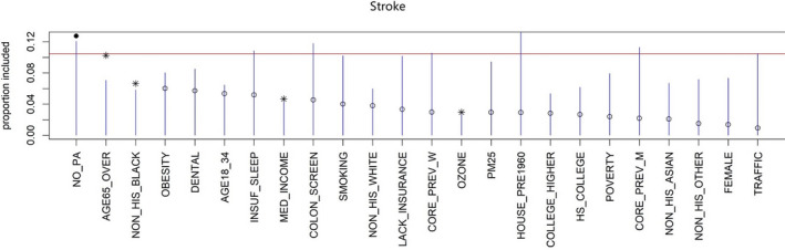
The blue lines are the threshold levels for variable selection procedure described in Figure 1. The red line represents the cutoff determined by a more stringent rule. Variables passing this threshold are displayed as solid dots. Variables that exceed the blue lines but not the red line are represented as asterisks. We select variables with either an asterisk or a solid dot. Open dots correspond to variables that are not selected.
To understand the synergistic or antagonistic effects of the chosen predictors, we further investigated the importance of variable interactions. Figure 4 shows the top 10 interaction terms computed from the BART model for the neighborhood‐level prevalence of stroke. The relative importance is most distinct for the interaction between the prevalence of leisure‐time physical activity and the percentage of adults ≥65 years of age.
Figure 4. The top 10 average interaction counts (termed as relative importance) for the neighborhood‐level prevalence of stroke, averaged over 25 BART model constructions.
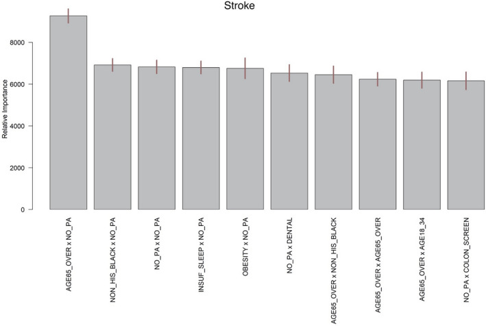
The segments atop the bars represent 95% confidence intervals. BART indicates Bayesian additive regression trees.
Comparing Operating Properties of BART, Boosting, and RFs in Variable Selection
We performed variable selection using the variable importance scores provided by boosting and RFs. Table 2 summarizes the RMSE, RMSE reduction per predictor, number of selected predictors, and the selected predictors for each of the 6 methods considered (4 tree based and 2 LR based), as described in the section Assessing Advantages of Machine Learning for Variable Selection. All 4 tree‐based methods had similar RMSEs with their respective selected predictors. BART selected the most parsimonious set of predictors and therefore had the largest RMSE reduction per predictor. The common predictors selected by all methods were the proportion of people who do not have leisure‐time physical activity, the share of non‐Hispanic Black people, the proportion of adults >65 years of age, median household income and interaction between the proportions of people who do not have leisure‐time physical activity and adults ≥65 years of age. Boosting and RFs tended to select more variables, some of which were highly correlated (see Table 2). Ozone was selected by BART‐Machine only.
Table 2.
RMSE Reduction, Number of Selected Predictors, and Selected Predictors by Each of 4 Tree‐Based Methods
| Methods | RMSE | RMSE Reduction per Predictor | Number of Predictors | Selected Predictors |
|---|---|---|---|---|
| BART | 0.48 | 0.15 | 6 |
NO_PA, NON_HIS_BLACK, AGE65_OVER, MED_INCOME, OZONE, NO_PA×AGE65_OVER |
| XGBoost | 0.48 | 0.11 | 8 | NO_PA, NON_HIS_BLACK, AGE65_OVER, MED_INCOME, OBESITY, SMOKING, INSUF_SLEEP, NO_PA×AGE65_OVER |
| gbm | 0.49 | 0.11 | 8 | NO_PA, NON_HIS_BLACK, AGE65_OVER, MED_INCOME, OBESITY, SMOKING, AGE18_34, NO_PA×AGE65_OVER |
| RFs | 0.47 | 0.09 | 11 | NO_PA, OBESITY, AGE65_OVER, NON_HIS_BLACK, DENTAL, INSUF_SLEEP, SMOKING, MED_INCOME, COLON_SCREEN, LACK_INSURANCE |
The Pearson correlation was −0.9 between DENTAL and LACK_INSURANCE (selected by RFs), 0.75 between SMOKING and INSUF_SLEEP (selected by XGBoost) and 0.84 between OBESITY and SMOKING (selected by gbm). LR‐StepWise retained 20 out of 24 predictors. Neither of the two LR methods had the capability to identify interactions. BART indicates Bayesian additive regression trees; gbm, gradient boosting machines; LR, linear regression; RFs, random forests; RMSE, root mean squared error; and XGBoost, Extreme Gradient Boosting.
The operating properties of all 6 methods considered are also provided in Figure 5.
Figure 5. RMSE, number of predictors and RMSE reduction per predictor for each of 6 methods: BART‐Machine, XGBoost, gbm, RF, stepwise LR variable selection and LR with all covariates.
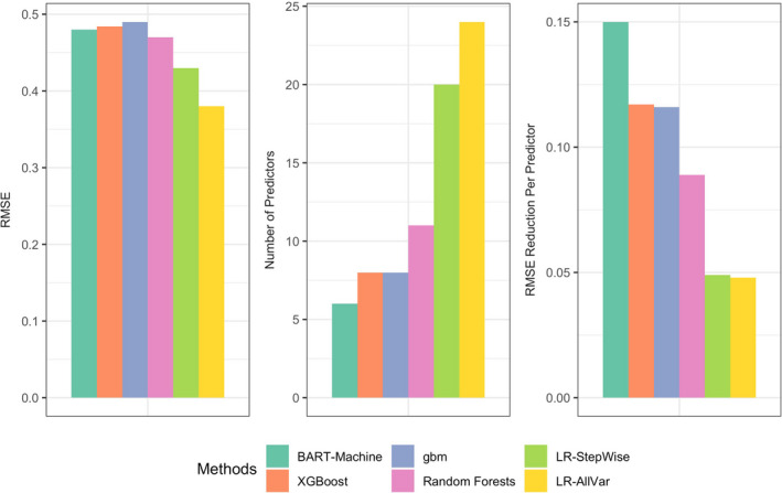
BART indicates Bayesian additive regression trees; gbm, gradient boosting machines; LR, linear regression; RFs, random forests; RMSE, root mean squared error; and XGBoost, Extreme Gradient Boosting.
Quantifying Exposure‐Outcome Associations
As machine learning methods are commonly limited by their “black‐box” nature, to strengthen findings from our machine learning models, we further fitted a Bayesian linear regression to evaluate the effects of key predictors and their interactions on the neighborhood‐level prevalence of stroke. Because BART showed the best predictive performance and best operating properties in variable selection, we used the key determinants identified by BART‐Machine. Figure 6 displays the point estimates and 95% credible intervals for each main and interaction effect.
Figure 6. Effect estimates and 95% credible intervals for 5 key predictors and 1 most important interaction.
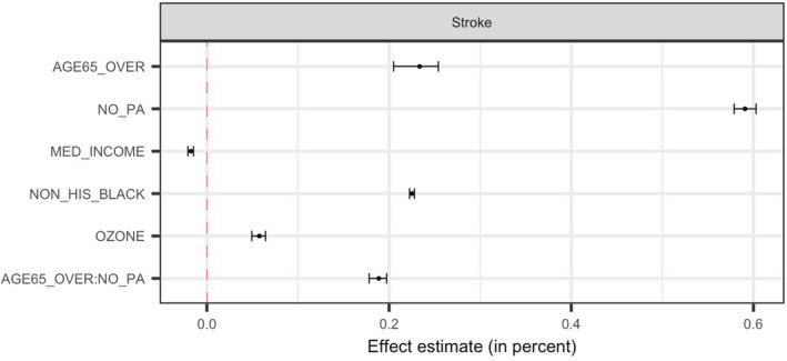
Effect estimates represent average changes in percent of stroke per 10% increase in AGE65_OVER, NO_PA or NON_HIS_BLACK, and per $100 000 increase in MED_INCOME and per 100 ppb (for the sake of legibility of the effect) increase in OZONE. AGE65_OVER indicates proportion of people who were ≥65 years old; MED_INCOME, Median household income in the past 12 months (in thousands); NO_PA, proportion of adults who had no leisure‐time physical activity; NON_HIS_BLACK, proportion of non‐Hispanic Black people; and OZONE, ozone level in air (ppb).
On average, a higher proportion of older residents and higher percentage of the population who are physically inactive in a neighborhood were associated with a higher prevalence of stroke at the neighborhood level. The neighborhoods with a larger share of non‐Hispanic Black people tended to have higher percentage of stroke. An increase of $100 000 in median household income was on average associated with a reduction of 0.19% in the neighborhood‐level prevalence of stroke. Ozone levels had an adverse effect on the prevalence of stroke—every 10 ppb increase in ozone was on average associated with 0.06% higher prevalence of stroke at the neighborhood level. No leisure‐time physical activity and age modified each other's effect. The positive sign of the interaction estimate indicates a synergistic effect of combined senior population and prevalence of physical inactivity.
Discussion
This study used the state‐of‐the‐art tree‐based machine learning approaches to identify and investigate major factors in predicting the neighborhood‐level prevalence of stroke, leveraging a large‐scale data set with information on unhealthy behaviors, prevention measures, sociodemographic status, and environmental factors garnered from more than 20 000 census tracts in 500 US major cities.
We identified key predictor variables for the prevalence of stroke at the neighborhood level. The results are consistent with known patient‐level risk factors. Neighborhoods with a higher proportion of older residents or physically inactive residents tended to have a higher prevalence of stroke. Ozone level was found to be adversely linked to the prevalence of stroke. Wealthier communities tended to have fewer strokes and neighborhoods with more non‐Hispanic Black people were associated with higher prevalence of stroke. We also found that older population structure and the lack of leisure‐time physical activity of a neighborhood together had a synergistic effect on the neighborhood‐level prevalence of stroke. It is worth noting that not all risk factors for stroke at the individual level, such as smoking and obesity, were ranked as having high importance scores in predicting neighborhood‐level stroke outcomes. One possible explanation is that different studies considered different candidate sets of predictors. We used wide‐ranging information across 4 domains. In addition, tree‐based machine learning methods like BART and XGBoost may be less likely to select highly correlated predictors than traditional LR because of their tree boosting modeling process.
Our study has several important implications related to public health and policy. Identifying important predictors of and how they jointly exert influence on neighborhood cardiovascular health would allow public health researchers and policymakers to have a deeper understanding of the drivers of neighborhood population health. Prevention measures such as lack of leisure‐time physical activity and environmental measures such as ozone level can provide important avenues for potential community‐level interventions. For example, community‐level interventions to engage residents in exercising, to improve air quality, and to build exercise‐friendly neighborhoods (eg, increasing walkability through parks and trails) may lead to fewer incidences of stroke in the communities. In addition, as the lack of physical activity exacerbated the effect of older age on stroke, indicated by the positive interaction effect, community‐based exercise promotion interventions that are aging friendly or with older adults in mind may alleviate overall prevalence of stroke.
Discovering the subset of predictors that are most influential on the outcomes is challenging, especially when the number of relevant predictors is sparse relative to the total number of available predictors and the fundamental relationships are nonlinear. Existing studies that have attempted to assess the relationships between neighborhood characteristics and cardiovascular health outcomes (often at the individual level) are limited in the scope of data source and analysis approaches. 34 Predictors are often restricted to a specific type (eg, behaviors) and selected a priori, risking “cherry picking.” As a result, these studies may overlook important determinants affecting cardiovascular health.
We considered a wide range of potential predictor variables from multiple sources for the neighborhood‐level prevalence of stroke, and compared the predictive performance of 4 tree‐based machine learning techniques and evaluated their abilities in variable selection. The predictors selected were largely consistent among the 4 methods. Moreover, BART‐Machine identified an additional important environmental predictor based on a principled permutation‐based inferential approach. The feature of “upblackboxing” interactions supplied by the machine learning algorithm provided us with an opportunity to gain insights into the effects of the major predictor variables, which are often ignored in studies using machine learning algorithms. We compared tree‐based approaches to linear regression with all predictors and with stepwise variable selection. The tree‐based approach, particularly BART‐Machine, distinguished a subset of most influential variables and top interactions, whereas the LR‐based procedure kept most variables (dropped only 4 variables) and was susceptible to selecting highly correlated variables. Coupled with the ranking of variable importance, our method can provide valuable guidance for targeted community‐based interventions. Finally, we complemented the machine learning modeling by conducting a Bayesian linear regression to quantify the effects of each major predictor and interaction on the neighborhood‐level prevalence of stroke.
The study has several limitations. First, behavioral measures available in the 500 Cities Data were small area estimations with their own uncertainties. Also, the prevalence of stroke only reflects the proportion of population who are alive and have a history of stroke, which may not accurately and completely reflect stroke incidence and severity of the disease and are subject to survivor bias. 35 However, the estimates provide the best available data for these small areas, and the approach has been well validated. 36 Second, given the nature of the cross‐sectional data and ecological design, the results do not bear causal interpretations.37 The identified neighborhood‐level factors of neighborhood‐level stroke prevalence can be potentially used to stimulate future research on causal relationships. Finally, while we included 24 predictors from 4 domains based on existing literature, the list is not exhaustive. Nonetheless, the study demonstrated the utility of a novel machine learning approach in identifying and understanding major determinants for stroke at the neighborhood level. Our results also have important implications in policymaking and designing intervention programs to improve population health.
Sources of Funding
This research was supported in part by award ME2017C3 9041 from the Patient‐Centered Outcomes Research Institute, a grant from the National Heart, Lung, and Blood Institute of the National Institutes of Health under Award Number R01HL141427, a grant from the National Institute on Minority Health and Health Disparities of the National Institutes of Health under Award Numbers R01MD013886, and 2 grants from the National Cancer Institute of the National Institutes of Health under Award Number R21CA235153 and R21CA245855. The contents of this article are solely the responsibility of the authors and do not necessarily represent the official views of the Patient‐Centered Outcomes Research Institute or National Institutes of Health.
Disclosures
None.
(J Am Heart Assoc. 2020;9:e016745 DOI: 10.1161/JAHA.120.016745.)
For Sources of Funding and Disclosures, see page 11.
References
- 1. Virani Salim S, Alonso A, Benjamin EJ, Bittencourt MS, Callaway CW, Carson AP, Chamberlain AM, Chang AR, Cheng S, Dellin FN, et al. Heart disease and stroke statistics—2020 update. Circulation. 2020;e139–e596. [DOI] [PubMed] [Google Scholar]
- 2. Yang W‐S, Wang X, Deng Q, Fan W‐Y, Wang W‐Y. An evidence‐based appraisal of global association between air pollution and risk of stroke. Int J Cardiol. 2014;307–313. [DOI] [PubMed] [Google Scholar]
- 3. Go AS, Mozaffarian D, Roger VL. Heart disease and stroke statistics—2014 update: a report from the American Heart Association. Circulation. 2014;e28–e292. [DOI] [PMC free article] [PubMed] [Google Scholar]
- 4. Bridgwood B, Lager KE, Mistri AK, Khunti K, Wilson AD, Modi P. Interventions for improving modifiable risk factor control in the secondary prevention of stroke. Cochrane Database Syst Rev. 2018;CD009103. [DOI] [PMC free article] [PubMed] [Google Scholar]
- 5. Boehme AK, Esenwa C, Elkind MSV. Stroke risk factors, genetics, and prevention. Circ Res. 2017;472–495. [DOI] [PMC free article] [PubMed] [Google Scholar]
- 6. Lee KK, Miller MR, Shah ASV. Air pollution and stroke. J Stroke. 2018;2–11. [DOI] [PMC free article] [PubMed] [Google Scholar]
- 7. Miller ET, King KA, Miller R, Kleindorfer D. FAST stroke prevention educational program for middle school students: pilot study results. J Neurosci Nurs. 2007;236–243. [DOI] [PubMed] [Google Scholar]
- 8. Marsden DL, Dunn A, Callister R, McElduff P, Levi CR, Spratt NJ. A home‐ and community‐based physical activity program can improve the cardiorespiratory fitness and walking capacity of stroke survivors. J Stroke Cerebrovasc Dis. 2016;2386–2398. [DOI] [PubMed] [Google Scholar]
- 9. Gong J, Chen X, Li S. Efficacy of a community‐based physical activity program KM2H2 for stroke and heart attack prevention among senior hypertensive patients: a cluster randomized controlled phase‐II trial. PLoS One. 2015;e0139442. [DOI] [PMC free article] [PubMed] [Google Scholar]
- 10. Mensah GA, Cooper RS, Siega‐Riz AM. Reducing cardiovascular disparities through community‐engaged implementation research: a National Heart, Lung, and Blood Institute workshop report. Circ Res. 2018;213–230. [DOI] [PMC free article] [PubMed] [Google Scholar]
- 11. Schüle SA, Bolte G. Interactive and independent associations between the socioeconomic and objective built environment on the neighbourhood level and individual health: a systematic review of multilevel studies. PLoS One. 2015;e0123456. [DOI] [PMC free article] [PubMed] [Google Scholar]
- 12. Osypuk TL, Ehntholt A, Moon JR, Gilsanz P, Glymour MM. Neighborhood differences in post‐stroke mortality. Circ Cardiovasc Qual Outcomes. 2017;e002547 10.1161/CIRCOUTCOMES.116.002547. [DOI] [PMC free article] [PubMed] [Google Scholar]
- 13. Kelly‐Hayes M. Influence of age and health behaviors on stroke risk: lessons from longitudinal studies. J Am Geriatr Soc. 2010;266–298. [DOI] [PMC free article] [PubMed] [Google Scholar]
- 14. Cities: local data for better health. Centers for Disease Control and Prevention; 2017. Available at: https://www.cdc.gov/500cities/index.htm. Accessed June 15, 2020. [Google Scholar]
- 15. American Community Survey 5-Year Data (2009-2018). United States Census Bureau; Available at: https://www.census.gov/data/developers/data-sets/acs-5year.html. Accessed June 15, 2020. [Google Scholar]
- 16. American FactFinder (AFF) . United States Census Bureau; Available at: https://data.census.gov/cedsci/. Accessed June 15, 2020. [Google Scholar]
- 17. Environmental Justice Mapping and Screening Tool. United States Environmental Protection Agency; Available at: https://www.epa.gov/ejscreen. Accessed June 15, 2020. [Google Scholar]
- 18. Chipman HA, George EI, McCulloch RE. BART: Bayesian additive regression trees. Ann Appl Stat. 2010;4:266–298. [Google Scholar]
- 19. Friedman JH. Greedy function approximation: a gradient boosting machine. Ann Stat. 2001;1189–1232. [Google Scholar]
- 20. Chen T, Guestrin C. XGBoost: a scalable tree boosting system. Proceedings of the 22nd ACM SIGKDD International Conference on Knowledge Discovery and Data Mining; 2016; San Francisco, CA, USA. [Google Scholar]
- 21. Breiman L. Random forests. Mach Learn. 2001;5–32. [Google Scholar]
- 22. Hastie T, Tibshirani R, Friedman JH. The Elements of Statistical Learning: Data Mining, Inference, and Prediction. 2nd ed New York: Springer; 2016. [Google Scholar]
- 23. Hill JL. Bayesian nonparametric modeling for causal inference. J Comput Graph Stat. 2011;217–240. [Google Scholar]
- 24. Hu L, Gu C, Lopez M, Ji J, Wisnivesky J. Estimation of causal effects of multiple treatments in observational studies with a binary outcome. Stat Methods Med Res. 2020;3218–3234. [DOI] [PMC free article] [PubMed] [Google Scholar]
- 25. Friedman J, Hastie T, Tibshirani R. Additive logistic regression: a statistical view of boosting. Ann Stat. 2000;337–407. [Google Scholar]
- 26. Bleich J, Kapelner A, George EI, Jensen ST. Variable selection for BART: an application to gene regulation. Ann Appl Stat. 2014;1750–1781. [Google Scholar]
- 27. Jiang H, Deng Y, Chen H‐S. Joint analysis of two microarray gene‐expression data sets to select lung adenocarcinoma marker genes. BMC Bioinformatics. 2004;81. [DOI] [PMC free article] [PubMed] [Google Scholar]
- 28. Dietrich S, Floegel A, Troll M. Random Survival Forest in practice: a method for modelling complex metabolomics data in time to event analysis. Int J Epidemiol. 2016;1406–1420. [DOI] [PubMed] [Google Scholar]
- 29. Hu L, Ji J, Li Y, Liu B, Zhang Y. Quantile Regression Forests to Identify Determinants of Neighborhood Stroke Prevalence in 500 Cities in the USA: Implications for Neighborhoods with High Prevalence. Journal of Urban Health. 2020:1–12. 10.1007/s11524-020-00478-y. [DOI] [PMC free article] [PubMed] [Google Scholar]
- 30. Kuhn M, Johnson K. Applied Predictive Modeling. 2nd ed New York: Springer; 2018. [Google Scholar]
- 31. Meaney C, Moineddin R. A Monte Carlo simulation study comparing linear regression, beta regression, variable‐dispersion beta regression and fractional logit regression at recovering average difference measures in a two sample design. BMC Med Res Methodol. 2014;14. [DOI] [PMC free article] [PubMed] [Google Scholar]
- 32. Merlo J, Wagner P, Ghith N, Leckie G. An original stepwise multilevel logistic regression analysis of discriminatory accuracy: the case of neighbourhoods and health. PLoS One. 2016;e0153778. [DOI] [PMC free article] [PubMed] [Google Scholar]
- 33. Gelman A, Carlin JB, Stern HS, Dunson DB, Vehtari A, Rubin DB. Bayesian Data Analysis. 3rd ed Boca Raton: Chapman and Hall/CRC; 2013. [Google Scholar]
- 34. Kershaw KN, Osypuk TL, Do DP, De Chavez PJ, Diez Roux AV. Neighborhood‐level racial/ethnic residential segregation and incident cardiovascular disease: the Multi‐Ethnic Study of Atherosclerosis. Circulation. 2015;141–148. [DOI] [PMC free article] [PubMed] [Google Scholar]
- 35. Hu L, Hogan JW. Causal comparative effectiveness analysis of dynamic continuous‐time treatment initiation rules with sparsely measured outcomes and death. Biometrics. 2019;695–707. [DOI] [PMC free article] [PubMed] [Google Scholar]
- 36. Zhang X, Holt JB, Yun S, Lu H, Greenlund KJ, Croft JB. Validation of multilevel regression and poststratification methodology for small area estimation of health indicators from the behavioral risk factor surveillance system. Am J Epidemiol. 2015;127–137. [DOI] [PMC free article] [PubMed] [Google Scholar]
- 37. Hu L, Hogan JW, Mwangi AW, Siika A. Modeling the causal effect of treatment initiation time on survival: Application to HIV/TB co‐infection. Biometrics. 2018;703–713. [DOI] [PMC free article] [PubMed] [Google Scholar]