Abstract
Lowering either the administered activity or scan time is desirable in PET imaging as it decreases the patient’s radiation burden or improves patient comfort and reduces motion artifacts. But reducing these parameters lowers overall photon counts and increases noise, adversely impacting image contrast and quantification. To address this low count statistics problem, we propose a cycle-consistent generative adversarial network (Cycle GAN) model to estimate diagnostic quality PET images using low count data.
Cycle GAN learns a transformation to synthesize diagnostic PET images using low count data that would be indistinguishable from our standard clinical protocol. The algorithm also learns an inverse transformation such that cycle low count PET data (inverse of synthetic estimate) generated from synthetic full count PET is close to the true low count PET. We introduced residual blocks into the generator to catch the differences between low count and full count PET in the training dataset and better handle noise.
The average mean error and normalized mean square error in whole body were −0.14% ± 1.43% and 0.52% ± 0.19% with Cycle GAN model, compared to 5.59% ± 2.11% and 3.51% ± 4.14% on the original low count PET images. Normalized cross-correlation is improved from 0.970 to 0.996, and peak signal-to-noise ratio is increased from 39.4 dB to 46.0 dB with proposed method.
We developed a deep learning-based approach to accurately estimate diagnostic quality PET datasets from one eighth of photon counts, and has great potential to improve low count PET image quality to the level of diagnostic PET used in clinical settings.
Keywords: PET, deep learning, low count statistics
1. Introduction
Positron emission tomography (PET) has become a widely employed imaging modality for disease diagnosis in oncology (Czernin et al 2007, Federman and Feig 2007), cardiology (Lee et al 2012, Youssef et al 2012) and neurology (Nordberg et al 2010, Andersen et al 2014). Due to degrading factors of positron range, non-collinear annihilation and scanner hardware design, PET images are associated with low count statistics (Votaw 1995). The diagnostic utility and quantitative accuracy critically depend on these count statistics (Lodge et al 2012), which mainly rely on scanner hardware configuration, patient attenuation, administered activity and scanning time (Sunderland and Christian 2015, Wickham et al 2017). Advances in nuclear medicine such as the widespread use of lutetium-based detectors and the clinical adoption of silicon photomultipliers (Nguyen et al 2015), time-of-flight (Karp et al 2008), resolution modeling (Leahy and Qi 2000) and noise regularization (Qi and Leahy 1999) have significantly increased signal-to-noise ratio (SNR). These improvements have led to some reductions in administered dose or scan time to maintain a similar SNR to images from instruments without these advancements (van der Vos et al 2017).
Protocol optimization based on patient body habitus (e.g. body mass index, weight) is often used to maintain consistency in noise texture with possible reductions in administered activity and scanning time for some patients (Wickham et al 2017). There is a continued desire to make further reductions in the administered activity to reduce radiation exposure, especially in pediatric populations that have higher lifetime cancer risk (Fahey et al 2017) and those who receive multiple scans for restaging and treatment monitoring (Chawla et al 2010, Fahey and Stabin 2014). Meanwhile, scanning time must be kept short for the consideration of motion control, patient comfort and scanner throughput (Fahey and Stabin 2014). The low count statistics caused by the limited administered activity and scanning time results in increased image noise, reduced contrast-to-noise ratio (CNR), and degraded image quality. Moreover, quantification errors resulting from low photon counts could increase bias in SUV measurements of up to 15% (Boellaard 2009). Therefore further improvements in hardware design and processing are needed to drive down administrative activity and scanning time without adversely affecting image quality and quantification.
Data-driven approaches such as machine learning- and deep learning-based methods have found success in a number of computer vision tasks and demonstrated great potential in the low count statistical problem of PET imaging. An et al trained multi-level canonical correlation analysis framework to estimate full dose PET images from its low dose counterpart, and refined the image quality iteratively with sparse representation (An et al 2016). MR images were also integrated into the sparse representation frameworks to provide anatomical and structural information for better estimation (An et al 2016, Wang et al 2016, 2017). The performances of these machine learning-based approaches depend on the handcraft features extracted based on prior knowledge, and well representing images with handcraft features is usually challenging. Moreover, small-patch-based methods tend to generate over-smoothed and blurred images resulting in loss of texture information. Recent applications of convolutional neural network (CNN) have been employed in denoising of low dose computed tomography and radiography (Chen et al 2017a, 2017b). 3D conditional generative adversarial network was utilized on [F-18] fluorodeoxyglucose (FDG) PET images to predict full dose (e.g. high count) PET images from low dose (e.g. low count) data and achieved superior performances to a CNN based method (Wang et al 2018). The method in Wang et al (2018) was applied on brain images with approximately one-quarter the counts of clinical protocol. Application of these data-driven approaches to brain data are often less complicated due to lower inter-patient anatomical variation in brain images comparing to that on whole-body images.
In this work, we propose a cycle-consistent generative adversarial network (Cycle GAN) to predict high-quality full count whole-body PET images from low count PET data. Cycle GAN architecture includes both a forward and reverse (i.e. cycle) training model on the low count and full count PET training data. This approach improves the GAN model’s prediction and uniqueness of the synthetic dataset. Residual blocks are also integrated to the architecture to better capture the difference of low count and full count images and enhance convergence. The proposed model was implemented and evaluated on whole-body FDG PET images, a more challenging dataset compared to brain images, with only 1/8th counts.
2. Method
2.1. Method overview
Figure 1 outlines the proposed full count PET synthesis algorithm, which consists of a training stage and a prediction stage. The full count PET image obtained with standard protocol is used as the deep learning-based target of the low count PET image. Due to the presence of noise, low count PET images demonstrate less texture information compared with full count PET images, thus training a transformation model from low count to full count (low-to-full) is an ill-posed inverse problem. To cope with this issue, a cycle-consistent adversarial network (Cycle GAN) is introduced to capture the relationship from low count to full count PET images while simultaneously supervising an inverse full count to low count (full-to-low) transformation model. The network can be thought of as two-pronged structure, simultaneously making itself better at both creating synthetic full count PET images and learning how to identify full count PET images. The input patch size for the Cycle GAN architecture was set to be 64 × 64 × 64. Each patch was extracted from full count and low count PET images by sliding the window with overlapping size of 18 × 18 × 18 to its neighboring patches. Individual components of the algorithm are outlined in further detail in the following sections.
Figure 1.
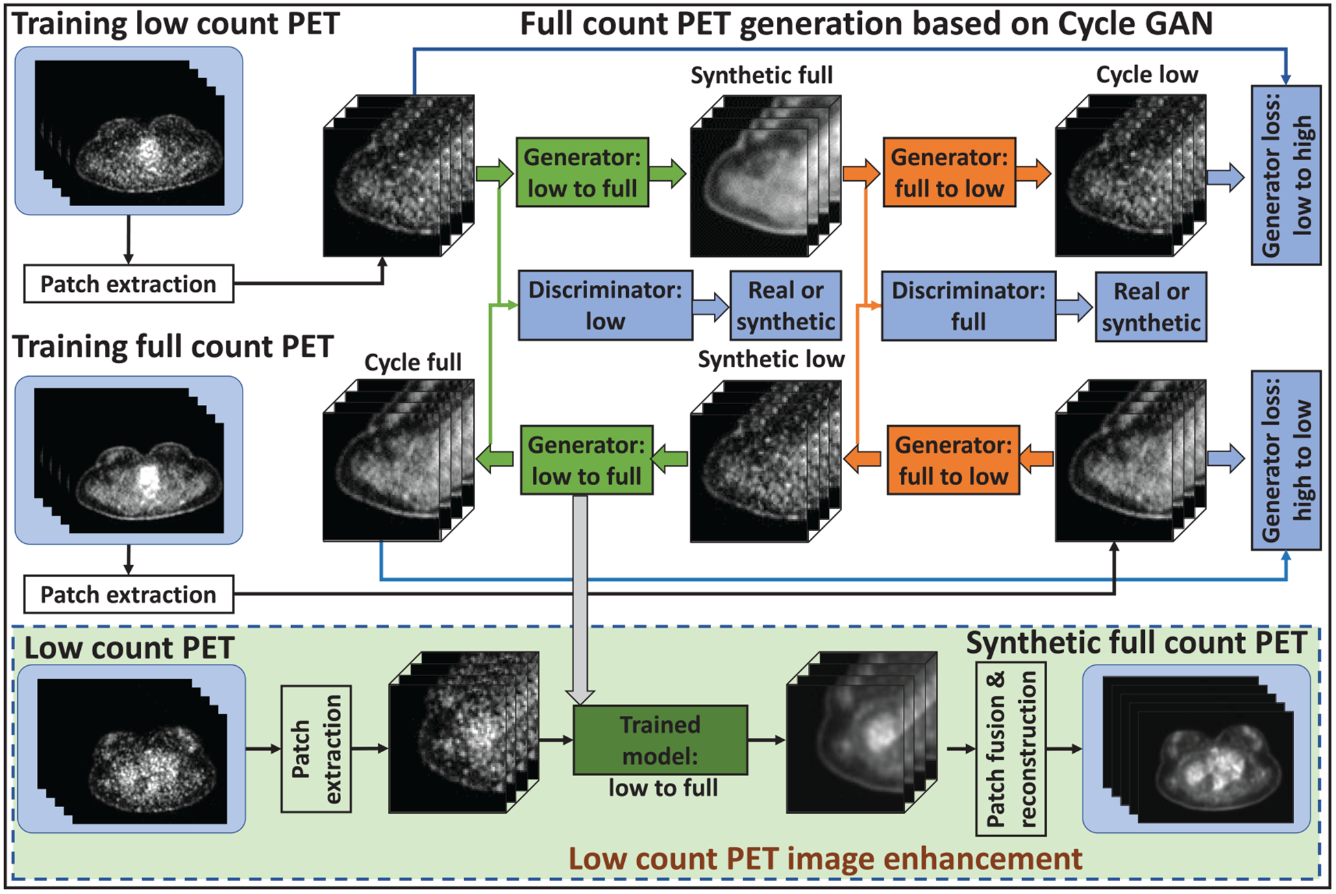
Schematic flow chart of the proposed method, full count PET synthesis based on cycle-consistent generative adversarial network. The top region of the figure represents the training stage, and the green-outlined region represents the test stage. During training, patches are extracted from paired low count and full count PET images. A convolutional neural network is used to down-sample the low count patch and the residual difference between the low count and the full count is minimized at this coarsest layer. The synthetic full count image is then up-sampled to its original resolution, and a discriminator is trained to learn the difference between this synthetic full count and the ground truth full count datasets. The inverse of this process is then carried out to generate the cycle low count PET image. Simultaneously to training the network that maps low count PET (to synthetic full count PET and then) to cycle low count PET, a complementary network is trained to transform ground truth full count PET to cycle full count PET. After training, a low count PET image can be fed into the generator (low-to-full) network to generate a synthetic full count PET image.
2.2. Network architecture
Figure 2 shows the detailed network architecture of generators and discriminators used in the proposed method. The generators learn a mapping from a source image to a target image. Since the source image and target image share similar structure, the residual network architecture was used to implement the generators to learn based on the residual image, i.e. the difference between the source and target image, rather than the entire images (Gao et al 2019, Harms et al 2019). Discriminator networks were introduced to evaluate the synthesized image. Typically, the generator’s objective is to increase the judgement error of the discriminative network, that is, fool the discriminator network by producing synthetic or cycle images that are indistinguishable to the input training images. The discriminators’ training objective is to decrease its judgement error and enhance the ability to differentiate true from synthetic images. In this work, the number of convolution layers in discriminator architecture is 9, where 8 layers are followed by batch normalization, the last 1 layer is followed by sigmoid function.
Figure 2.

Network architecture.
2.3. Cycle-consistent adversarial loss
The accuracy of both generator and discriminator networks depends on the design of their corresponding loss functions. The generator is optimized subject to
| (1) |
where G can be Glow-full (low-to-full generator) or Glow-full (full-to-low generator), λadv and λdist are weighting factors for adversarial loss and distance loss, respectively. is the adversarial loss function, which is formulated as,
| (2) |
where is the discriminator output for synthetic image and is the mean absolute difference between and a unitary mask, measuring the number of incorrectly generated pixels in the synthetic full count PET image. in equation (1) is the distance loss function composed of a compound loss function of mean p-norm distance (MPD) and gradient descent loss. The distance loss function is calculated as,
| (3) |
where GDL (, T) is the gradient descent loss function between the target image and the source image, described as below. ‖·‖p represents the p-norm,
| (4) |
for a vector x of length n. In this work, p is set to 1.5. This allows for a tradeoff between the sharpness preserved by the l1-norm and the blurring and voxel misclassification that have been observed when the l2-norm is used. The gradient descent loss function is calculated by
| (5) |
where i, j, and k denote pixels in the x, y, and z directions, denotes the square of 2-norm. Equation (5) minimizes the gradient magnitude difference between the target image and the source image, forcing the network to enhance edges which have strong gradients. As mentioned previously, the framework relies on training generators to perform both a low-to-full transformation and a full-to-low transformation. The generators are trained by a global generator loss function, called a cycle-consistent adversarial loss function,
| (6) |
where Isfull is the synthetic full count PET and is obtained by Isfull = Glow-full (Ilow). Ilow denotes the original low count PET. Iclow is the cycle low count PET and is obtained by Iclow = Gfull-low (Isfull). Islow is the synthetic low count PET and is obtained by Islow = Gfull-low (Ifull). Ifull denotes the original full count PET. Icfull is the cycle full count PET and is obtained by Icfull = Glow-full (Islow). λ is a regularization parameter for each component of equation (6). The discriminators are optimized in tandem with the generators according to
| (7) |
where MAD (Dfull (Isfull), 0) is defined the same as in equation (2), but a zero mask is used rather than a unit mask (all-ones matrix). The discriminator is designed to differentiate true images from synthetic ones. The zero masks in equation (7) reflect that the discriminator of a given image type (full count PET) should be able to find a synthetic image of the different type. On the other hand, the unit mask indicates that the discriminator should always identify a full count PET image. As mentioned above, the proposed framework relies on learning the bi-directional relationships between the source image and target image. This framework produces a model that is robust to noisy data or data that is compromised with artifacts. Given two images with similar underlying structures, the cycle-consistent adversarial network is designed to efficiently learn an intensity mapping from the source distribution to the target distribution, even if the relationship is ill posed nonlinear. The proposed framework learns this mapping based on residual images, or the difference between the low count and the full count PET images.
2.4. Evaluation and validation
A retrospective sample of 25 consecutive whole-body FDG oncology patient datasets were collected for model training and evaluation. An additional ten consecutive whole-body FDG oncology patient datasets were collected for model evaluation that were not used in the model training and validation. All PET data were acquired with Discovery 690 PET/CT scanner (General Electric) using a BMI-based administration protocol of either 370 MBq (BMI < 30) or 444 MBq (BMI ⩾ 30) followed by a 60 min uptake period. Emission data were collected based on BMI for 2.5 min (BMI ⩾ 25), 2 min (18.5 < BMI < 25) or 1.5 min (BMI ⩽ 18.5) for each bed position. Images were reconstructed with a 3D ordered-subset expectation maximization (OSEM) algorithm (3 iterations, 24 subsets) with time-of-flight and corrections for attenuation, scatter, randoms, normalization and deadtime (Iatrou et al 2004). A post-image Gaussian filter of 6.4 mm was applied to all images. The reconstruction matrix was 192 × 192 with a pixel size of 3.65 × 3.65 × 3.27 mm3. Low count PET data were created by histogramming the emission data to one-eighth the bed duration for all bed positions and reconstructing with the same OSEM algorithm parameters.
Whole brain, lung, heart, bilateral kidneys, liver, lesions and whole-body volumes of interest were delineated on CT images. The performance of proposed method was quantified with mean error (ME) (Botchkarev 2018), normalized mean square error (NMSE) (Lee et al 2019) and peak signal to noise ratio (PSNR) (Lei et al 2018a, Yang et al 2019) calculated for each contoured volume,
| (8) |
| (9) |
| (10) |
ME and NMSE are averaged over all voxels inside the contoured and whole body volume V. N is the total number of voxels inside the volume, and Ifull (i) is are the intensity values from ground truth full count PET, and I′ is those of low count PET or synthetic full count PET image. max(·) is the max intensity inside volume V. We also calculated normalized cross correlations (NCC) to quantify the intensity and structure similarity between full count PET and low count PET or synthetic full count PET. NCC (Lei et al 2018b) is defined as,
| (11) |
where mean(·) and std(·) calculate the mean intensity and standard deviation inside volume V.
Cycle GAN was built on top of the established model, GAN. To demonstrate the effectiveness of introducing cycle-consistent framework, we compared the performance of the proposed Cycle GAN model and U-Net and GAN model (Wang et al 2018) with leave-one-out cross validation and also on the dataset that are excluded from training, which is a hold-out test. Leave-one-out cross validation is used for evaluation of the proposed algorithm. In this evaluation method, we excluded one patient from each dataset when training the model, namely, 24 patients from total 25 patients were used for training the model. After training, the excluded patient’s images are used as test images. This procedure is repeated 25 times such that each patient is used as test patient for exactly once. The hold-out validation was also used. For this experiment, we used previous 25 patients as training data, and used additional 10 patients as test data. Our algorithm was implemented in Python 3.6 and Tensorflow with Adam gradient descent optimizer and were trained and tested on a NVIDIA Tesla V100 GPU with 32 GB of memory. The learning rate for Adam optimizer was set to 2 × 10⁻⁵. The batch size was set to 10. During training, 7.2 GB CPU memory and 27.6 GB GPU memory was used for each batch optimization. It takes about 12 min per 2000 iterations during training. In the testing, it takes about 2 min to generate an estimated full count PET image for one patient. The training was stopped after 150 000 iterations.
3. Results
3.1. Leave-one-out cross validation
Figure 3 shows a representative subject’s low count, full count, synthetic full count PET with U-NET (U-NET GAN), synthetic full count PET with GAN model (GAN PET) and synthetic full count PET with cycle GAN model (Cycle GAN PET). All three models suppress image noise and enhance image quality substantially compared to low count PET. Comparing to U-NET and GAN models, the proposed Cycle GAN method obtains better image quality and better matches in texture to the full count images. The improvements in Cycle GAN are particularly evident in organs of normal physiological update such as the brain, heart, liver and kidneys in figure 3. These similarities are also evident in figure 3(g) on a cranial-caudal profile comparison and the joint histograms in figure 4. As shown in figure 4, joint histogram with Cycle GAN shows a more constrict distribution towards line of identity, indicating better correlation to full count PET.
Figure 3.
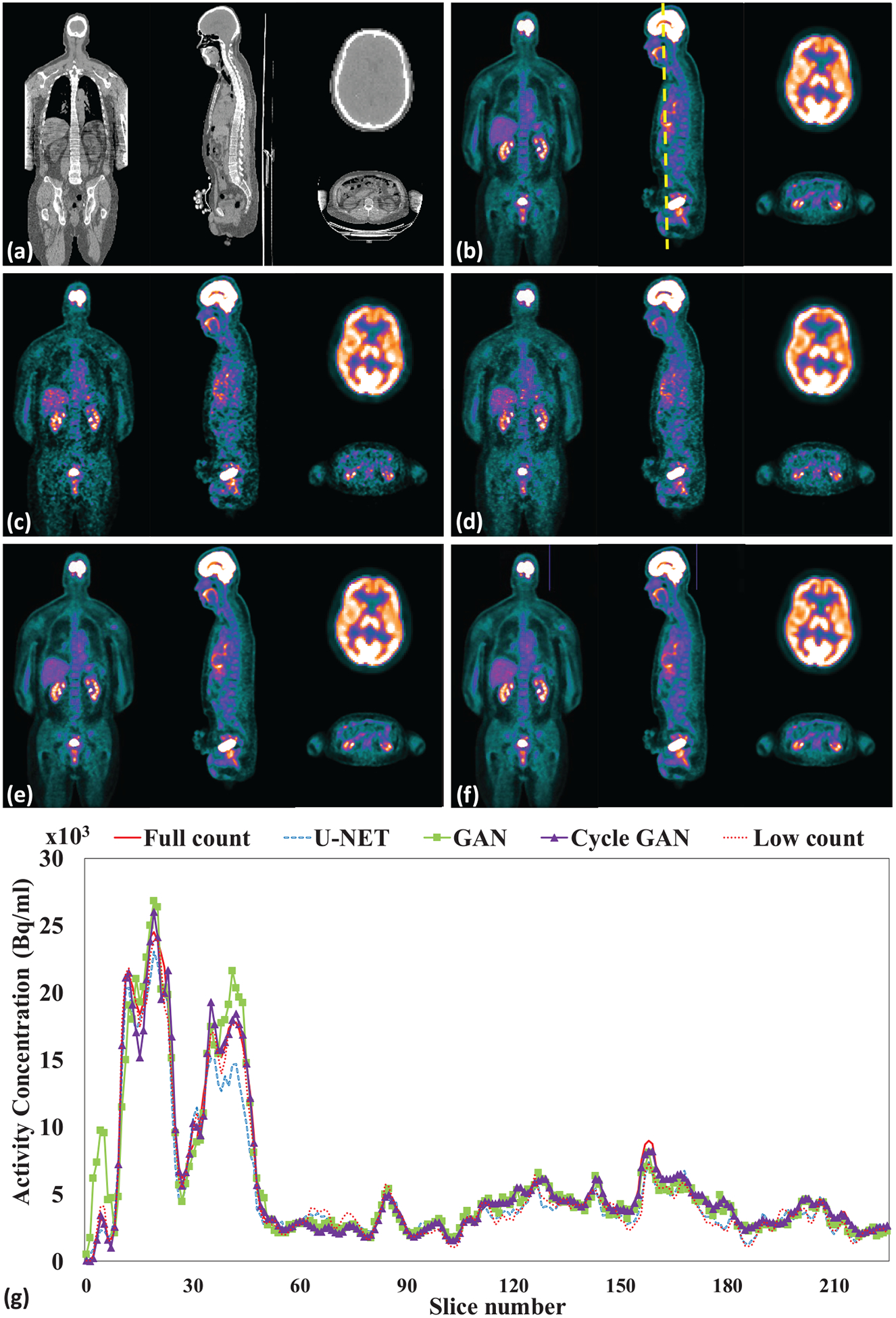
Leave-one-out cross validation. Images are (a) CT (b) full count PET (c) low count PET, (d) U-NET PET, (e) GAN PET, (f) Cycle GAN PET images on the coronal, sagittal and axial planes and (g) PET image profiles of low count, full count, U-NET, GAN and Cycle GAN PET. The dashed line on (b) indicates the position of a sagittal cranial-caudal profile displayed in (g). The brain axial PET images were displayed with brain window for better visualization, and all other were displayed with kidney window.
Figure 4.
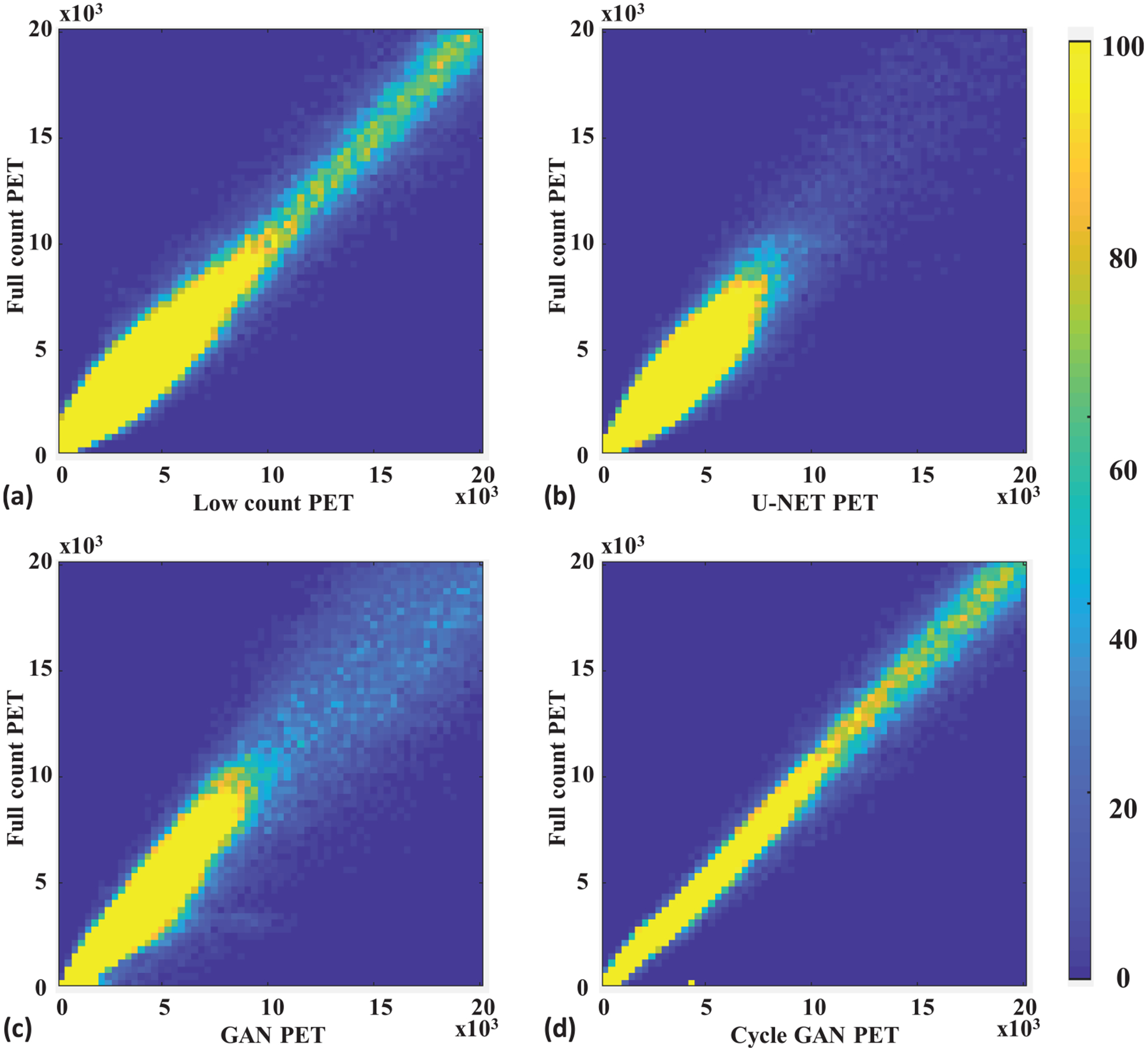
Leave-one-out cross validation. Joint histogram of full count PET with (a) low count, (b) U-NET, (c) GAN and (d) Cycle GAN PET. The x-axis of (a)–(d) is the pixel value of low count PET or synthetic full count PET generated by the U-NET, GAN, and the proposed Cycle GAN. The y -axis of (a)–(d) is the corresponding pixel value of full count PET. The color represents relative frequency in range of 0 to 100.
Table 1 presents the quantitative results of the leave-one-out cross validation. ME, NMSE, NCC and PSNR were calculated on low count PET, U-NET PET, GAN PET and Cycle GAN PET over full count PET images. Both ME and NMSE are improved to less than 1% with Cycle GAN model, comparing to 5.59% and 3.51% on the original low count images, 3.46% and 3.50% on GAN PET, 0.73% and 3.32% on U-NET PET. The PSNR is enhanced and the PSNR increased from 39.4 dB to 46.0 dB with Cycle GAN, and more modestly to 39.8 with GAN model and U-NET. Individual organ and whole-body contour results of the leave-one-out cross validation are presented in figure 5. U-NET, GAN and Cycle GAN reduced ME and NMSE, improved NCC and PSNR, while Cycle GAN shows superior performances on average in all metrics. The ME on the normal organs ranged from 1.3%–4.3% with U-NET, 0.9%–6.3% with GAN and 0.2%–2.4% with Cycle GAN. The ME on lesions was reduced from 9.6% to 6.1% with U-NET, 2.2% with GAN and to 1.3% with Cycle GAN. Similarly, the NMSE was reduced in range from 0.7%–5.1% to 1.9%–4.3% with U-NET, to 1.8%–3.4% with GAN and to 0.6%–1.6% with Cycle GAN. The correlation between low count PET and full count PET was also enhanced with the proposed method, and NCC range was increased from 0.709–0.962 to 0.962–0.992 with Cycle GAN. Image contrast, interns of PSNR range, improved both qualitatively and quantitatively from 22.5–29.1 dB to 22.0–29.1 dB with GAN and to 28.8–38.5 dB with Cycle GAN in normal organs. The PSNR in lesions improved from 19.1 dB to 19.6 dB for U-NET, to 22.0 dB for GAN and 29.6 dB for Cycle GAN.
Table 1.
Quantitative comparison between low count PET, U-NET PET, GAN PET and Cycle GAN PET on whole body with leave-one-out cross validation. Data are reported as mean ± STD.
| ME | NMSE | NCC | PSNR (dB) | |
|---|---|---|---|---|
| Low count | 5.59% ± 2.11 | 3.51% ± 4.14% | 0.970 ± 0.030 | 39.4 ±3.1 |
| U-NET | 0.73% ± 1.35% | 3.32% ± 0.74% | 0.971 ± 0.012 | 39.8 ± 2.3 |
| GAN | −3.46% ± 5.28% | 3.50% ± 2.75% | 0.970 ± 0.026 | 39.8 ± 3.7 |
| Cycle GAN | −0.14% ± 1.43% | 0.52% ±0.19% | 0.996 ± 0.002 | 46.0 ± 3.8 |
| P-value Cycle GAN versus Low count | <0.001 | <0.001 | <0.001 | <0.001 |
| P-value Cycle GAN versus GAN | 0.744 | <0.001 | <0.001 | <0.001 |
| P-value Cycle GAN versus U-NET | 0.001 | <0.001 | <0.001 | <0.001 |
Figure 5.
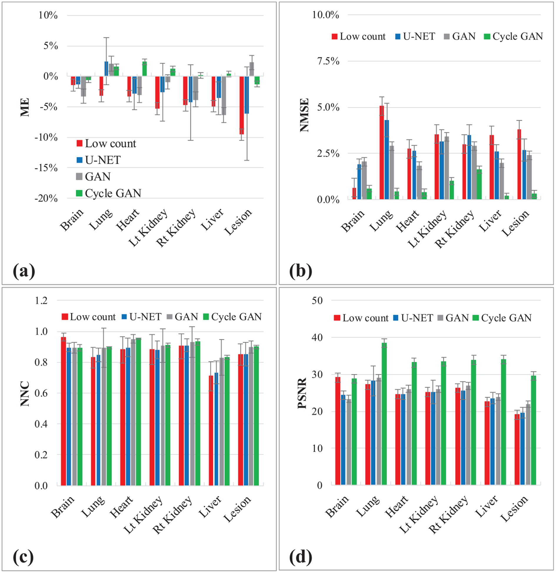
Leave-one-out cross validation. Figures show quantitative comparison between low count PET, U-NET PET, GAN PET and Cycle GAN PET, in terms of (a) ME, (b) NMSE, (c) NCC and (d) PSNR on normal organs and lesions. The error bar is standard deviation.
3.2. Performance validation on separate dataset
The performances of the proposed method were further evaluated on the dataset that are excluded from training. As illustrated in figure 6, U-NET, GAN and Cycle GAN suppress image noise, improve visual detectability and enhance the profiles. Cycle GAN performs better in all three views as illustrated in figures 6 and 7 show greater enhancement in profile comparison and histogram comparison. The quantitative results in figure 8 and table 2 both demonstrate better matching of Cycle GAN PET images with full count PET images, comparing to GAN PET.
Figure 6.
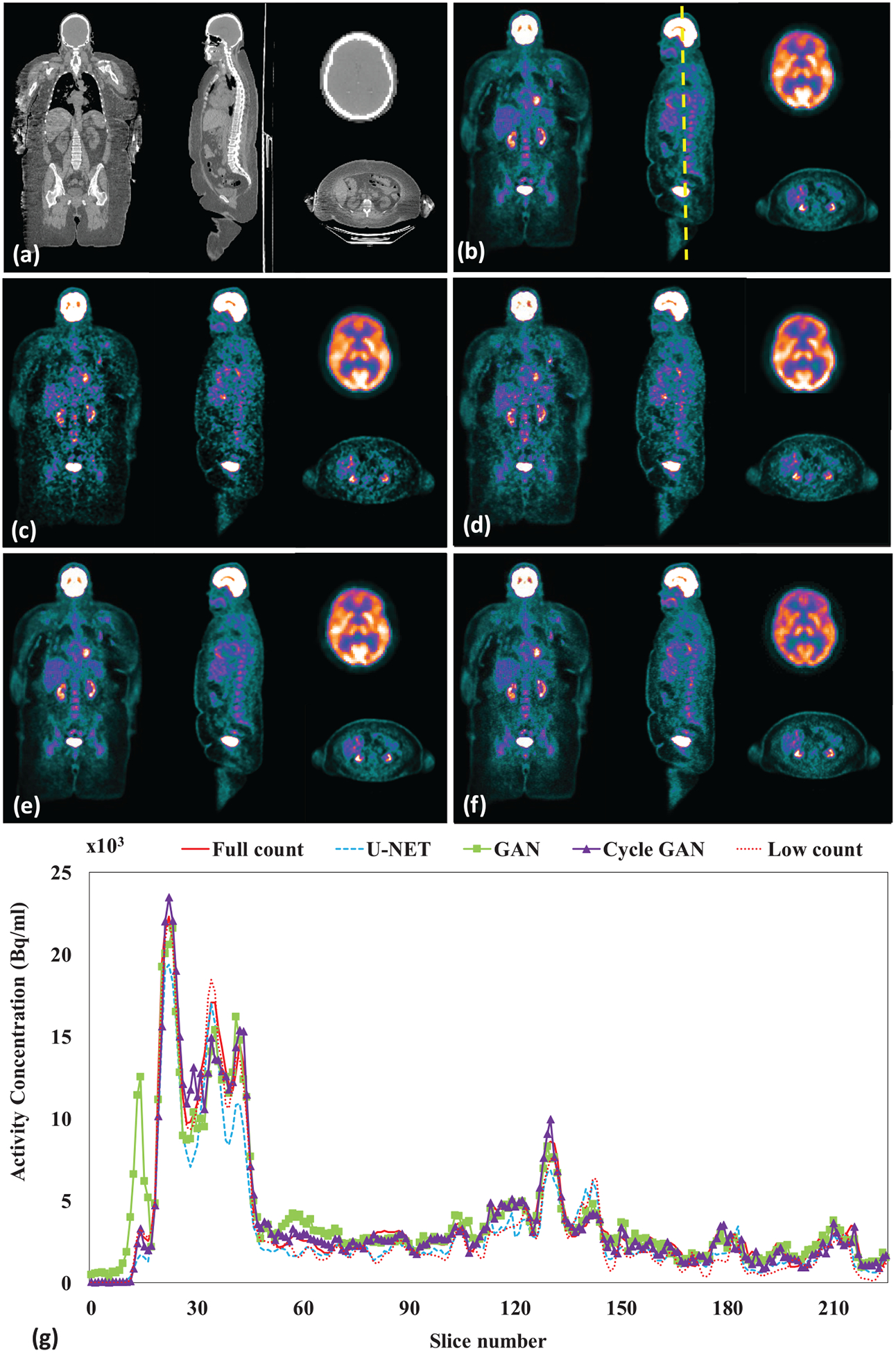
Hold-out validation. Images are (a) CT (b) full count PET (c) low count PET, (d) U-NET PET, (e) GAN PET, (f) Cycle GAN PET images on the coronal, sagittal and axial planes and (g) PET image profiles of low count, full count, U-NET, GAN and Cycle GAN PET. The dashed line on (b) indicates the position of a sagittal cranial-caudal profile displayed in (g). The brain axial PET images were displayed with brain window for better visualization, and all other were displayed with kidney window.
Figure 7.
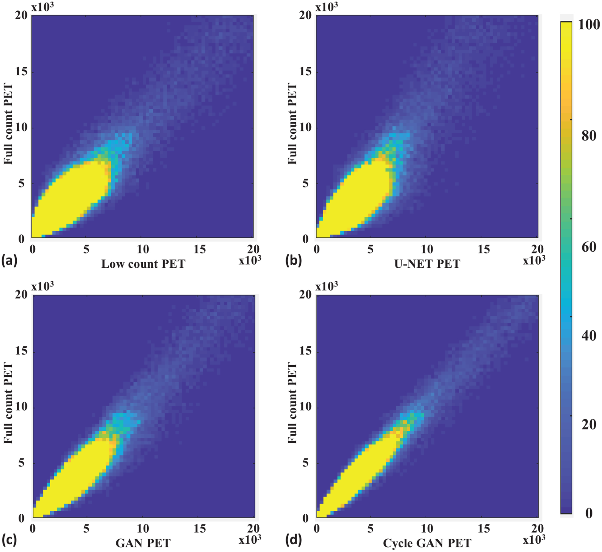
Hold-out validation. Joint histogram of full count PET with (a) low count, (b) U-NET, (c) GAN and (d) Cycle GAN PET. The x-axis of (a)–(d) is the pixel value of low count PET or synthetic full count PET generated by the U-NET, GAN, and the proposed Cycle GAN. The y -axis of (a)–(d) is the corresponding pixel value of full count PET. The color represents relative frequency in range of 0 to 100.
Figure 8.
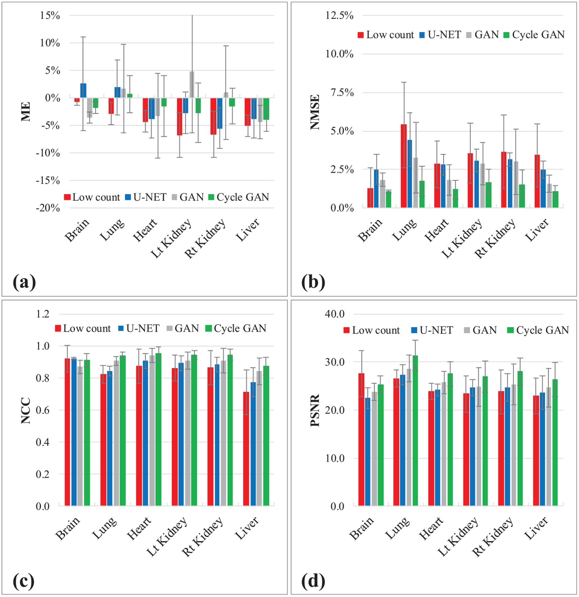
Hold-out validation. Figures show quantitative comparison between original low count PET, U-NET PET, GAN PET and Cycle GAN PET, in terms of (a) ME, (b) NMSE, (c) NCC and (d) PSNR on normal organs. The error bar is standard deviation.
Table 2.
Quantitative comparison between low count PET, U-NET PET, GAN PET and Cycle GAN PET with Hold-out validation. Data are reported as mean ± STD.
| ME | NMSE | NCC | PSNR (dB) | |
|---|---|---|---|---|
| Low count | 6.70% ± 4.10% | 4.11% ± 2.50% | 0.963 ± 0.023 | 38.1 ± 3.4 |
| U-NET | 1.03% ± 2.80% | 3.74% ± 0.97% | 0.967 ± 0.008 | 38.6 ± 2.1 |
| GAN | −1.4% ± 3.55% | 2.90% ± 0.99% | 0.975 ± 0.008 | 39.3 ± 4.0 |
| Cycle GAN | 0.16% ± 1.36% | 1.75% ± 0.66% | 0.984 ± 0.007 | 41.5 ± 2.5 |
| P-value Cycle GAN versus Low count | <0.001 | 0.004 | 0.004 | 0.001 |
| P-value Cycle GAN versus GAN | 0.290 | <0.001 | <0.001 | <0.001 |
| P-value Cycle GAN versus U-NET | 0.198 | <0.001 | <0.001 | 0.005 |
4. Discussion
In this work, we proposed a cycle-consistent generative adversarial network to predict high-quality full count PET images from low count PET data. GAN has demonstrated superior performances in generative image modeling compared to stand-alone CNN in medical imaging denoising of compromised data (Yang et al 2018, You et al 2018b). Due to the presence of noise in both input sources and output targets of the model training, it would be difficult to ensure the generator in GAN learns a meaningful mapping such that a unique output exists for a given input. The generator could create nonexistent features or collapse to a narrow distribution (You et al 2018a). Cycle GAN adds more constraint to the generator by introducing an inverse transformation in a circular manner. This more effectively avoids model collapse and better ensures the generator find a unique meaningful mapping. The above studies demonstrate improved performance of Cycle GAN over GAN in the low count PET problem.
Comparing to other bench mark studies, our method shows appealing performances. Wang et al incorporate both low dose PET and MR images in the training of a patch-based sparse representation framework to estimate full dose PET images achieving 1.3% NMSE in their brain PET image dataset (Wang et al 2016). Another study performed by the same group utilized 3D conditional generative adversarial networks to predict full dose PET images, and obtained around 2% NMSE on both normal organs and lesions (Wang et al 2018). These two studies were both performed on brain images, which present largely uniform and symmetric uptake, and do not suffer from complicated non-rigid motion artifacts observed in whole-body. For these reasons and others, the NMSE can be lower compared to peripheral organs with only modest improvements in this quantitative measure as demonstrated in our work. We reported NMSE in brain of 0.60% ± 0.24%, which agrees well with Wang et al and is comparable to our results in the peripheral organs and whole-body regions.
The inferior performance of our model in brain quantification was observed on the evaluation with the second dataset. No significant differences were found in our quantitative measures, and these findings may be due to a limited number of subjects (4 of 10) having their whole brain imaged. Considering that all subjects in this work are referred to PET based on a cancer diagnosis, brain is usually not a critical focus of their treatment. Further work will need to be performed to evaluate the clinical significance of this methodology on sensitivity and specificity compared to standard of care full count PET.
Standard protocols commonly calculate administered activity proportional to patient weight, but these protocols still result in compromised image quality on overweight patients. Masuda et al found that, when patient’s weight increased from 50 kg to 77 kg, doubling the radiation exposures or scanning time still generated degraded SNR (Masuda et al 2009). PET counts drop dramatically with increase of patient weight and attenuation. To maintain similar image quality, administered activity and scanning time must be increased significantly on overweighed patients to compensate for the loss of photon counts. The proposed method demonstrated superior performances to recover high quality PET images from 1/8 of standard counts and has potential to facilitate PET imaging on overweight patients.
With the recent introduction of total body PET, the large gain in sensitivity can reduce the overall scan duration to less than one minute (Rahmim et al 2019). We have shown that a deep learning approach with Cycle GAN can produce diagnostic quality images in 1/8th PET counts resulting in a whole-body scan duration of just under 2 min for 6 bed positions. The gain in apparent sensitivity could be utilized to further develop more sophisticated acquisition strategies such as dynamic whole-body acquisitions or delay imaging.
5. Conclusion
We developed a deep learning-based approach to accurately estimate diagnostic quality PET datasets from 1/8th of full count based on a cycle-consistent GAN with integrated residual blocks. The proposed deep learning-based approach has great potential to improve low count PET image quality to the level of diagnostic PET used in clinical settings. This approach can be used to substantially reduce the administered dose or scan duration while maintaining a high diagnostic quality.
Acknowledgments
This research was supported in part by the National Cancer Institute of the National Institutes of Health Award Number R01CA215718 and the Emory Winship Cancer Institute pilot grant.
References
- An L, Zhang P, Adeli h, Wang Y, Ma G, Shi F, Lalush DS, Lin W and Shen D 2016. Multi-level canonical correlation analysis for standard-dose PET image estimation IEEE Trans. Image Process 25 3303–15 [DOI] [PMC free article] [PubMed] [Google Scholar]
- Andersen FL, Ladefoged CN, Beyer T, Keller SH, Hansen AE, Hojgaard L, Kjaer A, Law I and Holm S 2014. Combined PET/MR imaging in neurology: MR-based attenuation correction implies a strong spatial bias when ignoring bone NeuroImage 84 206–16 [DOI] [PubMed] [Google Scholar]
- Boellaard R 2009. Standards for PET image acquisition and quantitative data analysis J. Nucl. Med 50 11S–20S [DOI] [PubMed] [Google Scholar]
- Botchkarev A 2018. Performance metrics (error measures) in machine learning regression, forecasting and prognostics: properties and typology IJIKM 14 45–76 [Google Scholar]
- Chawla SC, Federman N, Zhang D, Nagata K, Nuthakki S, McNitt-Gray M and Boechat MI 2010. Estimated cumulative radiation dose from PET/CT in children with malignancies: a 5-year retrospective review Pediatr. Radiol 40 681–6 [DOI] [PMC free article] [PubMed] [Google Scholar]
- Chen H, Zhang Y, Kalra MK, Lin F, Chen Y, Liao P, Zhou J and Wang G 2017a. Low-dose CT with a residual encoder-decoder convolutional neural network IEEE Trans. Med. Imaging 36 2524–35 [DOI] [PMC free article] [PubMed] [Google Scholar]
- Chen H, Zhang Y, Zhang W, Liao P, Li K, Zhou J and Wang G 2017b. Low-dose CT via convolutional neural network Biomed. Opt. Express 8 679–94 [DOI] [PMC free article] [PubMed] [Google Scholar]
- Czernin J, Allen-Auerbach M and Schelbert HR 2007. Improvements in cancer staging with PET/CT: literature-based evidence as of September 2006 J. Nucl. Med 48 78S–88S [PubMed] [Google Scholar]
- Fahey F and Stabin M 2014. Dose optimization in nuclear medicine Semin. Nucl. Med 44 193–201 [DOI] [PubMed] [Google Scholar]
- Fahey FH, Goodkind A, MacDougall RD, Oberg L, Ziniel SI, Cappock R, Callahan MJ, Kwatra N, Treves ST and Voss SD 2017. Operational and dosimetric aspects of pediatric PET/CT J. Nucl. Med 58 1360–6 [DOI] [PMC free article] [PubMed] [Google Scholar]
- Federman N and Feig SA 2007. PET/CT in evaluating pediatric malignancies: a clinician’s perspective J. Nucl. Med 48 1920–2 [DOI] [PubMed] [Google Scholar]
- Gao F, Wu T, Chu X, Yoon H, Xu Y and Patel B 2019. Deep residual inception encoder-decoder network for medical imaging synthesis IEEE J. Biomed. Health Inform ( 10.1109/JBHI.2019.2912659) [DOI] [PubMed] [Google Scholar]
- Harms J, Lei Y, Wang T, Zhang R, Zhou J, Tang X, Curran WJ, Liu T and Yang X 2019. Paired cycle-GAN-based image correction for quantitative cone-beam computed tomography Med. Phys 46 3998–4009 [DOI] [PMC free article] [PubMed] [Google Scholar]
- Iatrou M, Ross SG, Manjeshwar RM and Stearns CW 2004. A fully 3D iterative image reconstruction algorithm incorporating data corrections IEEE Symp. Conf. Record Nuclear Science (Rome, Italy) [Google Scholar]
- Karp JS, Surti S, Daube-Witherspoon ME and Muehllehner G 2008. Benefit of time-of-flight in PET: experimental and clinical results J. Nucl. Med 49 462–70 [DOI] [PMC free article] [PubMed] [Google Scholar]
- Leahy RM and Qi J 2000. Statistical approaches in quantitative positron emission tomography Stat. Comput 10 147–65 [Google Scholar]
- Lee D, Kim J, Moon W-J and Ye JC 2019. CollaGAN: collaborative GAN for missing image data imputation (arXiv:1901.09764)
- Lee WW et al. 2012. PET/MRI of inflammation in myocardial infarction J. Am. Coll. Cardiol 59 153–63 [DOI] [PMC free article] [PubMed] [Google Scholar]
- Lei Y. et al. MRI-based pseudo CT synthesis using anatomical signature and alternating random forest with iterative refinement model. J. Med. Imaging. 2018a;5:043504. doi: 10.1117/1.JMI.5.4.043504. [DOI] [PMC free article] [PubMed] [Google Scholar]
- Lei Y. et al. Magnetic resonance imaging-based pseudo computed tomography using anatomic signature and joint dictionary learning. J. Med. Imaging. 2018b;5:034001. doi: 10.1117/1.JMI.5.3.034001. [DOI] [PMC free article] [PubMed] [Google Scholar]
- Lodge MA, Chaudhry MA and Wahl RL 2012. Noise considerations for PET quantification using maximum and peak standardized uptake value J. Nucl. Med 53 1041–7 [DOI] [PMC free article] [PubMed] [Google Scholar]
- Masuda Y, Kondo C, Matsuo Y, Uetani M and Kusakabe K 2009. Comparison of imaging protocols for 18F-FDG PET/CT in overweight patients: optimizing scan duration versus administered dose J. Nucl. Med 50 844–8 [DOI] [PubMed] [Google Scholar]
- Nguyen NC, Vercher-Conejero JL, Sattar A, Miller MA, Maniawski PJ, Jordan DW, Muzic RF Jr, Su KH, O’Donnell JK and Faulhaber PF 2015. Image quality and diagnostic performance of a digital PET prototype in patients with oncologic diseases: initial experience and comparison with analog PET J. Nucl. Med 56 1378–85 [DOI] [PubMed] [Google Scholar]
- Nordberg A, Rinne JO, Kadir A and Langstrom B 2010. The use of PET in Alzheimer disease Nat. Rev. Neurol 6 78–87 [DOI] [PubMed] [Google Scholar]
- Qi J and Leahy RM 1999. A theoretical study of the contrast recovery and variance of MAP reconstructions from PET data IEEE Trans. Med. Imaging 18 293–305 [DOI] [PubMed] [Google Scholar]
- Rahmim A, Lodge MA, Karakatsanis NA, Panin VY, Zhou Y, McMillan A, Cho S, Zaidi H, Casey ME and Wahl RL 2019. Dynamic whole-body PET imaging: principles, potentials and applications Eur. J. Nucl. Med. Mol. Imaging 46 501–18 [DOI] [PubMed] [Google Scholar]
- Sunderland JJ and Christian PE 2015. Quantitative PET/CT scanner performance characterization based upon the society of nuclear medicine and molecular imaging clinical trials network oncology clinical simulator phantom J. Nucl. Med 56 145–52 [DOI] [PubMed] [Google Scholar]
- van der Vos CS, Koopman D, Rijnsdorp S, Arends AJ, Boellaard R, van Dalen JA, Lubberink M, Willemsen ATM and Visser EP 2017. Quantification, improvement, and harmonization of small lesion detection with state-of-the-art PET Eur. J. Nucl. Med. Mol. Imaging 44 4–16 [DOI] [PMC free article] [PubMed] [Google Scholar]
- Votaw JR 1995. The AAPM/RSNA physics tutorial for residents. Physics of PET RadioGraphics 15 1179–90 [DOI] [PubMed] [Google Scholar]
- Wang Y, Ma G, An L, Shi F, Zhang P, Lalush DS, Wu X, Pu Y, Zhou J and Shen D 2017. Semisupervised tripled dictionary learning for standard-dose PET image prediction using low-dose PET and multimodal MRI IEEE Trans. Biomed. Eng 64 569–79 [DOI] [PMC free article] [PubMed] [Google Scholar]
- Wang Y, Yu B, Wang L, Zu C, Lalush DS, Lin W, Wu X, Zhou J, Shen D and Zhou L 2018. 3D conditional generative adversarial networks for high-quality PET image estimation at low dose NeuroImage 174 550–62 [DOI] [PMC free article] [PubMed] [Google Scholar]
- Wang Y et al. 2016. Predicting standard-dose PET image from low-dose PET and multimodal MR images using mapping-based sparse representation Phys. Med. Biol 61 791–812 [DOI] [PubMed] [Google Scholar]
- Wickham F, McMeekin H, Burniston M, McCool D, Pencharz D, Skillen A and Wagner T 2017. Patient-specific optimisation of administered activity and acquisition times for 18F-FDG PET imaging EJNMMI Res. 7 3. [DOI] [PMC free article] [PubMed] [Google Scholar]
- Yang Q, Yan P, Zhang Y, Yu H, Shi Y, Mou X, Kalra MK and Wang G 2018. Low-dose CT image denoising using a generative adversarial network with Wasserstein distance and perceptual loss IEEE Trans. Med. Imaging 37 1348–57 [DOI] [PMC free article] [PubMed] [Google Scholar]
- Yang XF, Wang TH, Lei Y, Higgins K, Liu T, Shim H, Curran WJ, Mao H and Nye JA 2019. MRI-based attenuation correction for brain PET/MRI based on anatomic signature and machine learning Phys. Med. Biol 64 025001. [DOI] [PMC free article] [PubMed] [Google Scholar]
- You C et al. 2018a. CT super-resolution GAN constrained by the identical, residual, and cycle learning ensemble(GAN-CIRCLE) IEEE Trans. Med. Imaging ( 10.1109/TMI.2019.2922960) [DOI] [PMC free article] [PubMed] [Google Scholar]
- You C et al. 2018b. Structurally-sensitive multi-scale deep neural network for low-dose CT denoising IEEE Access 6 41839–55 [DOI] [PMC free article] [PubMed] [Google Scholar]
- Youssef G et al. 2012. The use of 18F-FDG PET in the diagnosis of cardiac sarcoidosis: a systematic review and metaanalysis including the Ontario experience J. Nucl. Med 53 241–8 [DOI] [PubMed] [Google Scholar]


