Semi-automated PIRADS scoring via mpMRI analysis

Abstract.

Purpose: Prostate cancer (PCa) is the most common solid organ cancer and second leading cause of death in men. Multiparametric magnetic resonance imaging (mpMRI) enables detection of the most aggressive, clinically significant PCa (csPCa) tumors that require further treatment. A suspicious region of interest (ROI) detected on mpMRI is now assigned a Prostate Imaging-Reporting and Data System (PIRADS) score to standardize interpretation of mpMRI for PCa detection. However, there is significant inter-reader variability among radiologists in PIRADS score assignment and a minimal input semi-automated artificial intelligence (AI) system is proposed to harmonize PIRADS scores with mpMRI data.

Approach: The proposed deep learning model (the seed point model) uses a simulated single-click seed point as input to annotate the lesion on mpMRI. This approach is in contrast to typical medical AI-based approaches that require annotation of the complete lesion. The mpMRI data from 617 patients used in this study were prospectively collected at a major tertiary U.S. medical center. The model was trained and validated to classify whether an mpMRI image had a lesion with a PIRADS score greater than or equal to PIRADS 4.

Results: The model yielded an average receiver-operator characteristic (ROC) area under the curve (ROC-AUC) of 0.704 over a 10-fold cross-validation, which is significantly higher than the previously published benchmark.

Conclusions: The proposed model could aid in PIRADS scoring of mpMRI, providing second reads to promote quality as well as offering expertise in environments that lack a radiologist with training in prostate mpMRI interpretation. The model could help identify tumors with a higher PIRADS for better clinical management and treatment of PCa patients at an early stage.

1. Introduction

Prostate cancer (PCa) is the most common solid organ cancer with the second highest cancer mortality rate among men in the United States.¹ PCa screening improves early detection of high-risk PCa and involves a digital rectal exam, a prostate-specific antigen test, transrectal ultrasound biopsy (TRUS bx), and multiparametric magnetic resonance imaging (mpMRI) scans.^2,3 The 4Kscore that involves serum biomarkers and clinical information may help detect aggressive PCa but does not spatially localize or grade these lesions.⁴ The TRUS procedure uses sound waves to create a video image of the prostate gland that is used to guide the biopsy needle. The TRUS bx cores are graded based on the underlying epithelial histopathology using a Gleason score (GS)⁵ and associated Gleason grade group.^6,7 However, TRUS bx is performed in blinded fashion (i.e., may not be able to localize suspected lesions) in the posterior periphery of the prostate with significant error rates for accurate cancer detection and staging. Multiple single and multicenter trials have now shown that mpMRI-targeted biopsy improves diagnosis with increased detection of clinically significant PCa (csPCa).^8–10 mpMRI was shown to significantly improve risk assessment, biopsy planning as in the PROMIS⁹ and PRECISION trials,¹¹ have the ability to differentiate PCa from normal tissue,¹² and to detect csPCa.¹³ Specifically, mpMRI parameters [such as apparent diffusion coefficient (ADC)] are shown to be correlated with more aggressive GS ($\mathrm{GS}>7$).¹⁴ MR-targeted biopsy now enable precise sampling of the most aggressive Prostate Imaging-Reporting and Data System (PIRADS) region of interest (ROI) targets with decreased false positives and negative when compared to traditional systematic biopsy.^15,16

The PIRADS system is an attempt to standardize mpMRI interpretation and is a qualitative Likert-based 1 to 5 scale with higher values indicating higher mpMRI PCa suspicion.^7,12,17 The PIRADS score is assigned based on primarily on diffusion weighted imaging in the peripheral prostate zone and T2 weighted imaging in the central transitional zone, and prior studies have shown that lesions with higher PIRADS scores have a higher overall percentage of csPCa.^18–20 The PIRADS score is usually reported as part of the radiology report associated with each mpMRI study. This process of scoring requires knowledge of the latest iteration of the scoring criteria (PIRADS v2.1),²¹ by expert radiologists trained in prostate MRI interpretation at tertiary care centers.^22,23 However, many clinical centers worldwide are without access to radiologists with expertise in interpreting prostate mpMRI scans.²⁴ Expertise in prostate mpMRI interpretation could also affect the consensus between different readers. Studies have shown marginal inter-reader agreement in assignment of PIRADS v2 scores among expert radiologists²⁵ with higher consensus at higher PIRADS scores compared to lower scores.²⁶ Smith et al.²⁶ showed that the overall inter-reader readability was poor to moderate (kappa = 0.24 comparing four readers) and ratings even varied within the same reader over time (kappa = 0.43 to 0.67). Chen et al.²⁷ showed that there is moderate PIRADS v2 inter-reader readability but with an ability to predict csPCa.

An automated or semi-automated PIRADS scoring system could be beneficial to the PCa screening process because it would reduce the reliance on specifically trained radiologists and could improve the consistency of scoring. There is only one study to our knowledge that has automated the PIRADS v2 scoring system directly from mpMRI data.²⁸ Sanford et al.²⁸ utilized a pre-trained convolutional neural network (CNN) to classify mpMRI data between two PIRADS classes, i.e., PIRADS 2,3 versus PIRADS 4,5. Their cohort included 196 patients with PIRADS 2 or higher. Bounding boxes derived from manually annotated lesion contours were fed into CNN with a ResNet backbone. The input images are three channels: T2, ADC, and B-value diffusion weighted (BVAL) images. The authors report achieving an accuracy of 60% at the patient level using the slice with largest diameter of each lesion.

In addition to automating the PIRADS scoring process, other studies have attempted to predict the biopsy results using only screening imaging. These studies include a deep learning-based model to classify csPCa,²⁹ a model to classify prostate lesions as with or without GS 4,³⁰ and a model to jointly detect and classify PCa.³¹ These studies aimed to predict the severity in patients whose PIRADS scores indicated the need for a biopsy, so they serve as the next step in the clinical pipeline after PIRADS scoring. While pathologic grading is critical, PIRADS scoring remains a key step in a patient’s diagnostic workup, signaling both the presence of a suspicious ROI as well as its aggressivity.

In this study, we demonstrate a model that predicts the PIRADS score using mpMRI data. The model would help distinguish between mpMRI lesions with a PIRADS score greater than or equal to 4. This criterion to classify lesions with a PIRADS score greater than or equal to 4 is based on prior literature, where studies have shown, higher PIRADS scores are associated with a higher percentage of csPCa.^18–20 This deep learning model could be deployed clinically to assist a radiologist in the assessment and scoring of mpMRI data as part of PCa detection by augmenting the existing screening pipeline.

2. Problem Definition

With the increasing rate of incidence of PCa in men in the U.S, there has been more attention over the last decade focused on streamlining the clinical diagnostic and decision-making pathway. The PIRADS v2 and 2.1 scores were developed by the American College of Radiology PIRADS committee to standardize interpretation of mpMRI data for PCa detection. PIRADS v2 scoring is an additional step in the radiologist’s clinical workflow and naturally requires effort, time, and experience. The deep learning models proposed here are designed to assist the radiologist in PIRADS v2 scoring of a patient’s lesion. This model could augment the existing clinical workflow for PCa diagnosis. Our model could assist in identifying lesions with higher mpMRI lesion suspicion scores (PIRADS) and help in clinically deciding the course of action for PCa patients. These models, if validated, could reduce the radiologist’s reading time and workload as well as limiting the variability in scoring. The proposed model could make PIRADS scoring accessible to patients where abdominal radiology expertise is not available locally. In this paper, we show that our model is annotation-efficient in terms of the input to the model as well a sensitivity analysis for the input seed point.

3. Data

The initial study cohort included 1371 prospectively acquired 3-Tesla mpMRI studies from 1179 patients performed according to a standardized protocol at a U.S. tertiary referral center from June 2011 to May 2018 prior to MRI-targeted biopsy. All data were used for this work under the approval of the University of California, Los Angeles (UCLA) institutional review board (UCLA IRB#16-001361).

3.1. Inclusion and Exclusion Criteria

The inclusion criteria for the data included: availability of the mpMRI sequences T2, ADC, and BVAL, availability of the ROI masks annotated by expert radiologists at UCLA, and a valid PIRADS score assigned. Studies were excluded due to various irregularities such as corrupt image file (1), missing mpMRI sequence (70), missing ROI (2), multiple ROIs (356), no valid PIRADS score (270), ROI annotation irregularities (28), and T2 image dimension mismatch with the ROI mask (1). Follow-up studies of patients (26) were also removed from the dataset to ensure there is no information leak between the training, validation, and testing phases of the models as well as to remove any potential bias toward patients with more images. After satisfying the inclusion/exclusion criteria, the final cohort consisted of 617 patients.

3.2. Image Pre-Processing

The spatial resolution of the mpMRI sequences was $256\times 256\times 60$. The MRI data were resampled to an isotropic resolution, where the voxel spacing for each of the mpMRI sequences is 0.664 mm in the $x$, $y$, and $z$ directions. N4 bias field correction was applied as an MRI pre-processing step.³² The pixel intensity of the mpMRI sequences which are in different scales are rescaled to values in the range of 0 to 255.

3.3. Input Data Specification

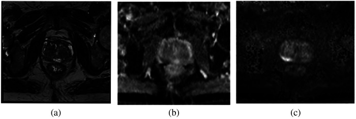
Figure 1 shows sample mpMRI sequences T2, ADC, and BVAL. Although T2 has the highest anatomical resolution, the other sequences capture lesion attributes that assist the PIRADS scoring algorithm.¹⁷ The different mpMRI sequences of a given patient at a given time are typically expected to be in close alignment, so no registration was performed. Further, empirically we did not see any added benefit of including registration in our processing pipeline. This decision is addressed in more detail in Sec. 6. The data fed into the 2D models (described in Sec. 3.4) have three channels, one slice selected from T2, ADC, and BVAL. The slice was chosen from each volume as the slice with the largest ROI area.

Fig. 1.

Sample data with the different mpMRI sequences: (a) T2, (b) ADC, and (c) BVAL.

3.4. Data Preparation

All studies used in this work had a PIRADS v2 score or a UCLA score assigned clinically by an expert genitourinary radiologist. The UCLA score, developed at the University of California, Los Angeles is quantitative scoring system from 1 to 5 predating the initial PIRADS v1 score and had similar performance to the qualitative PIRADS v2 score in terms of detection, grading csPCa.³³ Each study was assigned a class label based on its clinical score: class 1 with scores 2 or 3 and class 2 with scores 4 or 5. Approximately 66% (407/617) of studies were assigned to class 1 and the rest to class 2. The previous study by Sanford et al.²⁸ used as an external benchmark used this similar PIRADS-based dichotomization for their study. A 10-fold cross-validation is used to train, validate, and test the two proposed models.

4. Methods

4.1. Model Definition

The two different types of models developed and evaluated in this paper are described here.

4.1.1. ROI model

The first model requires as input, the mpMRI data and its associated ROI mask annotated by an expert radiologist.

4.1.2. Seed point model

The second model requires the mpMRI data and a single seed point to approximate the location of the ROI’s center.

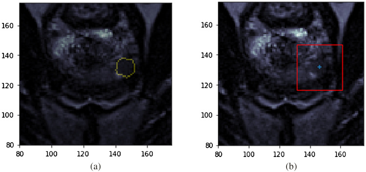
The ROI model is also included in this paper to compare the effect of minimal input (as in the case of the seed point model) on model performance. Sample input data used for both models are seen in Fig. 2. The figure on the left shows a cropped T2 slice with the radiologist’s ROI annotation as a yellow contour superimposed, which is the input to the ROI model. The figure on the right shows the input data for the seed point model. The blue plus denotes the single seed point required as input. The centroid of the lesion in the MRI slice where the ROI is largest was selected to simulate the single-click seed point. In practice, this seed point will be chosen by the radiologist as the approximate center for a suspicious region. The model then generates a patch of size $30\times 30\text{pixels}$ based on this seed point. The patch size was selected empirically.

Fig. 2.

Sample inputs into the models. (a) Corresponding radiologist annotated ROI mask (contour in yellow) on the T2 slice for the ROI model. (b) T2 slice with the single seed point marked by a blue plus and the red bounding box indicates the $30\times 30$ patch selected based on that center for seed point model. Images shown are cropped to improve visualization.

We also performed data augmentation on the input to both models with translation in $x$ and $y$ directions of 5 pixels each, horizontal and vertical flips, and random zooming in the range of [0.7, 1.3], to increase the robustness of the model. The three-channel images are centered to the mean that the pre-trained ImageNet³⁴ model was trained with.

4.2. Network Architecture

VGG-16³⁵ is utilized as the backbone architecture for our proposed deep learning models. The network is loaded with pre-trained weights³⁶ from the ImageNet dataset.³⁴ The fully connected layers at the end of the model are removed, and a new dense layer is attached to the top of the network with a sigmoid activation function. Another dense layer serves as the binary classifier between the PIRADS scores 2, 3 and 4, 5. Binary cross-entropy was utilized here as the loss function and is seen below:³⁷

$$L=-\frac{1}{m}\sum _{i=1}^m[y_i\log (p_i)+(1-y_i)\log (1-p_i)],$$ (1)

where $m$ defines the number of images in the entire training set, $y_i$ is class label for study $i$, and $p_i$ is the predicted probability of a sample belonging to class 1.

Figure 3 shows the pipeline of the proposed deep learning models. The Keras framework^37,38 with Tensorflow^39,40 as the backend was primarily used to implement, train, and test these models. The Scikit-learn library was used to implement the different performance metrics.⁴¹

Fig. 3.

The proposed deep learning pipeline for the ROI model and the seed point model. The models utilize the VGG-16 architecture for feature extraction. The input data are the 3-channel mpMRI data cropped based on the ROI mask or the single seed point. The output of the model is binary—class 1 (PIRADS 2, 3) or class 2 (PIRADS 4, 5).

4.3. Model Training

The model is trained in two stages on the prostate data. The first stage involves freezing all the layers of the CNN and training the dense layers. The second stage involves fine-tuning only the last two convolutional blocks of the CNN as well as the recently trained dense layers. The accuracy measure was used to monitor performance during training and validation over each epoch.

4.4. Hyperparameter Optimization

The hyperparameters of the deep network were optimized by minimizing the training and validation loss based on a grid search of key model hyperparameters. The performance curves were monitored during training and validation. Key model hyperparameters that were tuned include the optimizer (Adam, SGD, RMSprop), learning rate (2e-3 to 1e-5).

For the ROI model, the optimized hyperparameters were an Adam optimizer⁴² with a learning rate of 0.001 in stage 1 and with a learning rate of 0.00002 in the fine-tuning stage of the model. For the seed point model, the optimized hyperparameters used were an Adam optimizer with learning rate 0.0002 in stage 1 and 0.00002 in the fine-tuning stage of the model.

Some other hyperparameters that were tuned include dropout level,⁴³ batch size, training, and fine-tuning epochs. Experiments were done with and without dropout and regularization. We use $L2$ regularization with dropout of 0.1 for the ROI model and $L2$ regularization with no dropout for the seed point model. A batch size of 8 for training and validation for the ROI model and 32 for the seed point model are utilized.

4.5. Implementation

The first stage of training for ROI model is carried out for 25 epochs and the last two convolutional blocks are fine-tuned for another 15 epochs. The seed point model is trained for 60 epochs and then similarly fine-tuned for 30 epochs. Early stopping was used to train the models. The model hyperparameters mentioned earlier were tuned based on training and validation performance. The models where the performance converged with minimal overfitting and higher train/validation accuracy were taken as optimal. The overfitting was monitored based on how well the trained models generalized to the validation data.

4.6. Model Testing

4.6.1. Performance metrics

We evaluate the model by means of the calculated area under the curve based on the receiver-operator characteristic (ROC-AUC) and the precision-recall (PR-AUC) curves via 10-fold cross-validation. Other metrics presented are accuracy, precision, recall, and F1 metrics. These metrics are computed with the threshold obtained by optimizing Youden’s index from the ROC curve.⁴⁴ The performance was averaged and is presented along with their standard deviations.

4.6.2. Sensitivity analysis

The impact of the seed point selected on the prostate MRI is evaluated based on a sensitivity analysis experiment. The seed point for this analysis is generated based on randomly choosing values from a normal distribution by means of standard deviations from 1 through 10. The performance for this sensitivity analysis was based on the ROC-AUC score.

4.6.3. Statistical significance tests

Statistical tests were carried out to compare both of our models to each other as well as each with the external benchmark. The Delong test,⁴⁵ a paired non-parametric test was used to compare our models. The $Z$-test for one proportion,⁴⁶ an unpaired parametric test, was used to compare each of our models with the benchmark.

5. Results

The ROI model and seed point model are the two models proposed in this study. The results obtained are also contrasted with the external benchmark model.

5.1. Model Evaluation

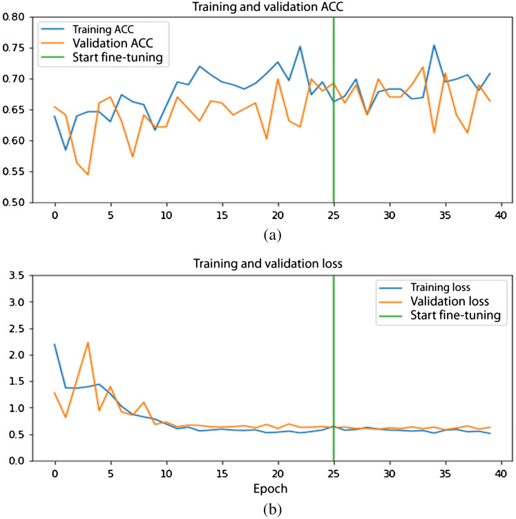
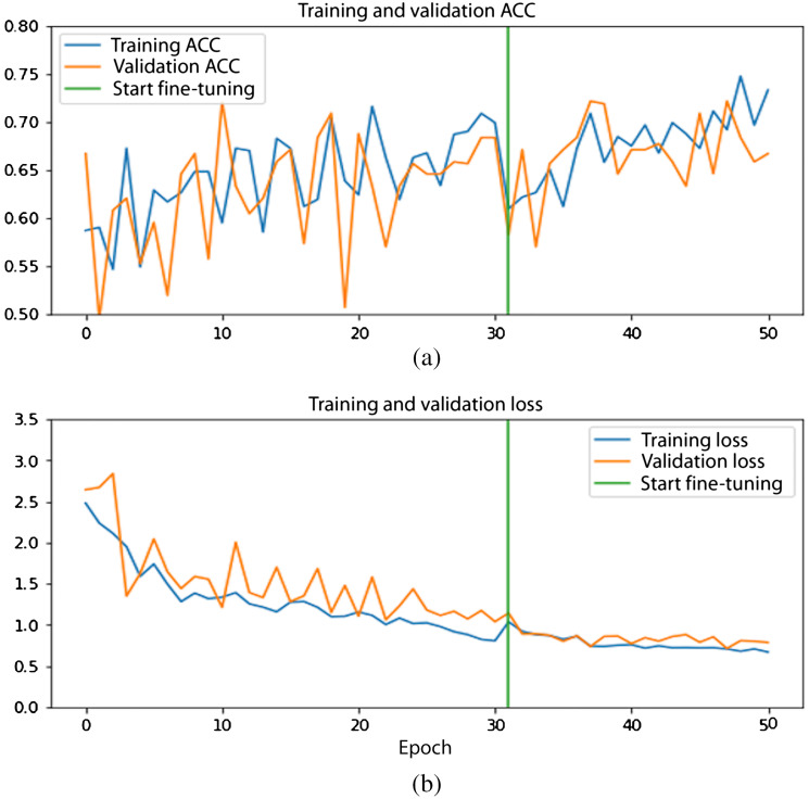
The validation curves of the ROI model and the seed point model for one of the folds from the 10-fold cross-validation are shown in Figs. 4 and 5.

Fig. 4.

Performance curves for the ROI model: (a) accuracy curves and (b) loss curves. Training (orange) and validation (blue) curve. Green line indicates start of fine-tuning.

Fig. 5.

Performance curves for seed point model: (a) accuracy curves and (b) loss curves. Training (orange) and validation (blue) curves. Green line indicates start of fine-tuning.

The loss curves show a gradual decrease during stage 1 of training and the trend continues with fine-tuning. Likewise, the accuracy curves for both models are seen to be increasing with higher epochs.

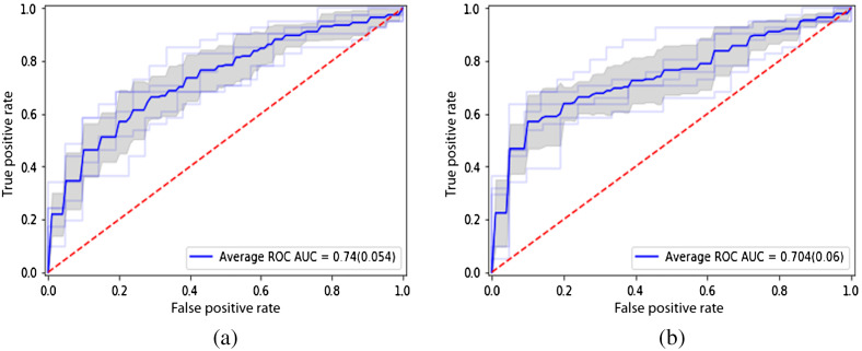
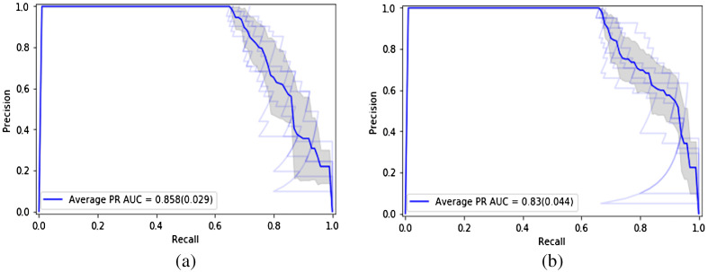
The ROC curves of the two models are seen in Fig. 6. The average ROC-AUC values achieved are 0.744 and 0.704 over the 10-fold cross-validation runs for the ROI model and seed point model, respectively. The PR curves are shown in Fig. 7. The average PR-AUC values are 0.858 and 0.830 for the two models, respectively.

Fig. 6.

ROC curves of the deep learning models: (a) with ROI model and (b) seed point model.

Fig. 7.

PR curves of the deep learning models: (a) with ROI model and (b) seed point model.

The performance of the two deep learning models proposed are compared with different metrics as shown in Table 1. The standard deviations over the different runs are documented in the table in parenthesis. The seed point model achieves average accuracy, precision, and recall values of 0.654, 0.888, and 0.558, respectively. The ROI model achieves average accuracy, precision, and recall values of 0.686, 0.880, and 0.619, respectively. A threshold determined by Youden’s index was used to measure the performance metrics for both models.

Table 1.

Performance metrics for the two deep learning models (ROI model and seed point model) with a 10-fold cross-validation.

	ROI model	Seed point model
Average ROC-AUC (SD)	0.744 (0.05)	0.704 (0.06)
Average PR-AUC (SD)	0.860 (0.03)	0.830 (0.04)
Average accuracy (SD)	0.686 (0.08)	0.654 (0.07)
Average precision (SD)	0.880 (0.06)	0.888 (0.07)
Average recall (SD)	0.619 (0.17)	0.558 (0.16)
Average F1 (SD)	0.708 (0.10)	0.666 (0.11)

5.2. Sensitivity Analysis

The sensitivity analysis experiment involves choosing random seed points at different standard deviations as seen in Table 2. The experiments are run using a 10-fold cross-validation to statistically show the robustness of the model. The effect of the variations in the seed point on the performance of the seed point model is measured in terms of the average ROC-AUC and the related standard deviations.

Table 2.

Sensitivity analysis shows seed point model is resilient to variations in the seed point with standard deviation.

Standard deviation (in $x$ and $y$ each (pixels)	Standard deviation (in $x$ and $y$ each (mm)	Average ROC-AUC for seed point model (SD)
0	0	0.704 (0.06)
1	0.664	0.694 (0.05)
2	1.328	0.696 (0.05)
3	1.992	0.671 (0.08)
4	2.656	0.652 (0.07)
5	3.32	0.671 (0.06)
6	3.984	0.647 (0.08)
7	4.648	0.623 (0.06)
8	5.312	0.612 (0.06)
9	5.976	0.622 (0.06)
10	6.64	0.618 (0.07)

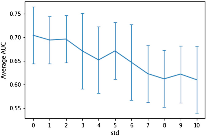
These results from the tables are visualized in Fig. 8, where the standard deviations are visualized as error bars at each value. The seed point model is seen to be relatively stable initially and the performance decreases for increasing values of standard deviation.

Fig. 8.

Visualization of the sensitivity analysis results from Table 2 ($y$-axis: average AUC over 10 cross-validation folds and the error bars indicate the corresponding standard deviations, $x$-axis: standard deviations from 1 through 10).

5.3. Model Comparison

The Delong paired statistical test shows that there is no statistical significance between our two models ($p=0.274$). The $Z$-test shows both of our proposed models significantly outperform the external benchmark ($p=0.032$ and $p=0.00003$ for the seed point and ROI models, respectively). It is important to note our ROI and seed point models with accuracies of 0.654 and 0.686, respectively, outperform the external benchmark accuracy of 0.60.

6. Discussion and Limitations

The model presented in this study both outperformed the existing methods for automating PIRADS scoring of prostate MRI. In Sec. 5, we presented results from two models to assist radiologists in PIRADS scoring of mpMRI data. The ROI model with the ROI annotation as input achieved an average ROC-AUC of 0.744 and seed point model with a single seed point achieved an average ROC-AUC of 0.704. It is interesting to note that the performance of seed point model requiring only a single seed point on the prostate MRI data is only 5% lower in terms of ROC-AUC. The ROI model achieves an average PR-AUC of 0.860 and the seed point model an average PR-AUC of 0.830. The statistical tests show that the performance of the model is not affected when the input ROI annotation is reduced from a full pixel-wise mask to just a single-pixel seed point. This indicates that our model could still be useful with minimal physician input. The models presented in this paper are based on a cohort of 617 patients. Our external benchmark, proposed by Sanford et al.,²⁸ reported an accuracy of 0.60. Both of our models significantly outperform the benchmark.

A sensitivity analysis is carried out to demonstrate the effect of the variations in the seed point selected on the prostate mpMRI volume. The experiments show that for smaller standard deviations the performance of the model is relatively stable. Increasing standard deviation further shows a drop in the seed point model’s performance (Fig. 8). For higher standard deviations, the resultant ROIs are unrealistically far from the lesion with many going outside the prostate boundary.

Studies have shown that there is inter-reader variability usually inherent in the PIRADS scoring system, which is a possible limitation. A larger dataset inclusive of data labeled by multiple radiologists would help minimize this issue. A future direction includes extending this work to a regression model to predict individual PIRADS scores. Further, we would like to fully automate the prediction to remove the requirement for even the seed point. It is also known that sometimes MRI underestimates the lesion contour. We plan to utilize whole mount histopathology data along with MRI as a way to improve this. We note that the different mpMRI sequences in our dataset were acquired at the same time for each of our patients, resulting in them being well-aligned. It is possible that clinical protocols in other institutions may result in alignment issues that need to be addressed through registration, which could be evaluated in future studies. The patch size used in this work was determined by means of empirical experiments. This value may be specific to our dataset, so future work should evaluate how this parameter varies across datasets from multiple clinics using different acquisition parameters.

7. Conclusions

Our results show that the seed point and ROI models were successful in classifying mpMRI data based on the clinically assigned PIRADS scores. The performance of our models does not degrade when using only a simulated single click seed point as input versus the full pixel-wise ROI annotation. We also show that our model is robust to small variations in the selection of the single MRI seed point. Our models significantly outperform the known benchmark and are trained on a dataset larger relative to theirs. In clinical practice, the seed point model could enable the development of clinical tools that would assist the radiologist in PIRADS scoring. This would help in reducing the reading time, and the workload of the radiologists by help shifting focus on more critical cases. The model could assist in identifying prostate mpMRI lesions PIRADS scores greater than or equal to 4. The models proposed could also help in reducing variability in the PIRADS scoring by automating the rule-based system with some oversight from the radiologist.

Biographies

Nikhil J. Dhinagar, PhD, is a postdoctoral scholar at the University of California, Los Angeles (UCLA). He received his PhD and MS degrees in electrical engineering from Ohio University. His research interests include image processing, computer vision, image analysis, machine learning, and deep learning.

William Speier, PhD, is an assistant professor at the UCLA and co-director of the Computational Diagnostics Laboratory. He received a master’s degree in computer science from Johns Hopkins University and his doctorate in biomedical engineering from UCLA. He is currently involved in several areas of research, including medical image analysis, natural language processing, and brain–computer interfaces.

Karthik V. Sarma, MS, is an MSTP fellow at the David Geffen School of Medicine at UCLA and a student in the UCLA Computational Diagnostics Laboratory. He received his undergraduate degree in computer science from California Institute of Technology and his master’s degree in bioengineering from UCLA. His research focuses on the application of image analysis and artificial intelligence to the medical domain, with a focus on prostate MRI.

Alex Raman is a medical student at the Western University of Health Sciences and an aspiring interventional radiologist. He has a background in software engineering and machine learning, having worked as a software developer for UCLA Health and having completed his master’s in bioinformatics from UCLA. His goal is to improve human at the patient level by integrating advanced technologies into patient care.

Adam Kinnaird MD, PhD, FRCSC, is an assistant professor at the University of Alberta. He received his doctorate in experimental medicine from the University of Alberta in 2018. He completed fellowship training at the UCLA in imaging, targeted biopsy, and focal therapy for prostate cancer (PCa) in 2020. He is an expert in PCa imaging and image-guided therapies as well as cancer metabolism.

Steven S. Raman, MD, is a professor of radiology, urology, and surgery at UCLA and director of the prostate IDx program, dedicated to improving PCa diagnostics. He received his MD with highest distinction from USC in 1993. He is an expert in abdominal imaging and image-guided interventions for prostate and other cancers.

Leonard S. Marks, MD, is a professor of urology at UCLA. He is inaugural holder of the Dekernion Endowed Chair in urology. His area of expertise is in the use of imaging to guide prostate biopsy for diagnosis of PCa and partial gland ablation for treatment. He was graduated AOA from the University of Texas Medical Branch and in 2018 received the Ashbel Smith Distinguished Alumnus award.

Corey W. Arnold, PhD, is an associate professor at UCLA and the director of the Computational Diagnostics Lab (CDx). He holds appointments in the Departments of Radiology, Pathology, Electrical and Computer Engineering, and Bioengineering. He received his PhD and MS degrees from UCLA, and his BS degree from the University of Wisconsin, Madison. His areas of research include machine learning, medical image analysis, computational phenotyping, and multi-modal disease modeling.

Disclosures

No conflicts of interest, financial or otherwise, are declared by the authors.

References

- 1.Siegel R. L., Miller K. D., Jemal A., “Cancer statistics, 2020,” CA. Cancer J. Clin. 70(1), 7–30 (2020). 10.3322/caac.21590 [DOI] [PubMed] [Google Scholar]
- 2.Grossman D. C., et al. , “Screening for prostate cancer,” J. Am. Med. Assoc. 319(18), 1901 (2018). 10.1001/jama.2018.3710 [DOI] [PubMed] [Google Scholar]
- 3.Walsh P., “Guide to surviving prostrate cancer,” 4th ed., Grand Central Life and Style; (2018). [Google Scholar]
- 4.Punnen S., Pavan N., Parekh D. J., “Finding the wolf in sheep’s clothing: the 4Kscore is a novel blood test that can accurately identify the risk of aggressive prostate cancer,” Rev. Urol. 17(1), 3–13 (2015). [PMC free article] [PubMed] [Google Scholar]
- 5.Gleason D. F., “Histologic grading of prostate cancer: a perspective,” Hum. Pathol. 23(3), 273–279 (1992). 10.1016/0046-8177(92)90108-F [DOI] [PubMed] [Google Scholar]
- 6.Epstein J. I., et al. , “The 2014 International Society of Urological Pathology (ISUP) consensus conference on Gleason grading of prostatic carcinoma definition of grading patterns and proposal for a new grading system,” Am. J. Surg. Pathol. 40(2), 244–252 (2016). 10.1097/PAS.0000000000000530 [DOI] [PubMed] [Google Scholar]
- 7.Sarkar S., Das S., “A review of imaging methods for prostate cancer detection,” Biomed. Eng. Comput. Biol. 7(Suppl. 1), 1–15 (2016). 10.4137/BECB.S34255 [DOI] [PMC free article] [PubMed] [Google Scholar]
- 8.Sonn G. A., Margolis D. J., Marks L. S., “Target detection: magnetic resonance imaging-ultrasound fusion-guided prostate biopsy,” Urol. Oncol. 32(6), 903–911 (2014). 10.1016/j.urolonc.2013.08.006 [DOI] [PMC free article] [PubMed] [Google Scholar]
- 9.Ahmed H. U., et al. , “Diagnostic accuracy of multi-parametric MRI and TRUS biopsy in prostate cancer (PROMIS): a paired validating confirmatory study,” Lancet 389(10071), 815–822 (2017). 10.1016/S0140-6736(16)32401-1 [DOI] [PubMed] [Google Scholar]
- 10.Ahdoot M., et al. , “MRI-targeted, systematic, and combined biopsy for prostate cancer diagnosis,” N. Engl. J. Med. 382(10), 917–928 (2020). 10.1056/NEJMoa1910038 [DOI] [PMC free article] [PubMed] [Google Scholar]
- 11.Kasivisvanathan V., et al. , “MRI-targeted or standard biopsy for prostate-cancer diagnosis,” N. Engl. J. Med. 378(19), 1767–1777 (2018). 10.1056/NEJMoa1801993 [DOI] [PMC free article] [PubMed] [Google Scholar]
- 12.Peng Y., et al. , “Quantitative analysis of multiparametric prostate MR images: differentiation between prostate cancer and normal tissue and correlation with Gleason score—a computer-aided diagnosis development study,” Radiology 267(3), 787–796 (2013). 10.1148/radiol.13121454 [DOI] [PMC free article] [PubMed] [Google Scholar]
- 13.Fütterer J. J., et al. , “Can clinically significant prostate cancer be detected with multiparametric magnetic resonance imaging? A systematic review of the literature,” Eur. Urol. 68(6), 1045–1053 (2015). 10.1016/j.eururo.2015.01.013 [DOI] [PubMed] [Google Scholar]
- 14.Nagarajan R., et al. , “Correlation of Gleason scores with diffusion-weighted imaging findings of prostate cancer,” Adv. Urol. 2012, 374805 (2012). 10.1155/2012/374805 [DOI] [PMC free article] [PubMed] [Google Scholar]
- 15.Elkhoury F. F., et al. , “Comparison of targeted vs systematic prostate biopsy in men who are biopsy naive: the prospective assessment of image registration in the diagnosis of prostate cancer (PAIREDCAP) study,” JAMA Surg. 154(9), 811–818 (2019). 10.1001/jamasurg.2019.1734 [DOI] [PMC free article] [PubMed] [Google Scholar]
- 16.Yacoub J. H., et al. , “Imaging-guided prostate biopsy: conventional and emerging techniques,” RadioGraphics 32(3), 819–837 (2012). 10.1148/rg.323115053 [DOI] [PubMed] [Google Scholar]
- 17.Weinreb J. C., et al. , “PI-RADS prostate imaging—reporting and data system: 2015, version 2,” Eur. Urol. 69(1), 16–40 (2016). 10.1016/j.eururo.2015.08.052 [DOI] [PMC free article] [PubMed] [Google Scholar]
- 18.Felker E. R., et al. , “Prostate cancer risk stratification with magnetic resonance imaging,” Urol. Oncol. 34(7), 311–319 (2016). 10.1016/j.urolonc.2016.03.001 [DOI] [PMC free article] [PubMed] [Google Scholar]
- 19.Chamie K., et al. , “The role of magnetic resonance imaging in delineating clinically significant prostate cancer,” Urology 83(2), 369–375 (2015). 10.1016/j.urology.2013.09.045 [DOI] [PMC free article] [PubMed] [Google Scholar]
- 20.Bassett M., “New research shows PI-RADS version 2 effective in prostate cancer diagnosis,” RSNA, 2018, https://www.rsna.org/en/news/2018/september/pi-rads-prostate-cancer-diagnosis
- 21.American College of Radiology, “Prostate imaging-reporting and data system,” Version 2.1, 2019, www.acr.org/-/media/ACR/Files/RADS/Pi-RADS/PIRADS-V2-1.pdf?la=en.
- 22.Jensen C., “Prostate cancer diagnosis using magnetic resonance imaging—a machine learning approach,” PhD Dissertation, Aalobourg University, Denmark (2018).
- 23.Barentsz J., et al. , “Prostate imaging-reporting and data system version 2 and the implementation of high-quality prostate magnetic resonance imaging,” Eur. Urol. 72(2), 189–191 (2017). 10.1016/j.eururo.2017.02.030 [DOI] [PubMed] [Google Scholar]
- 24.Gupta R. T., Spilseth B., Froemming A. T., “How and why a generation of radiologists must be trained to accurately interpret prostate mpMRI,” Abdom. Radiol. 41(5), 803–804 (2016). 10.1007/s00261-016-0745-4 [DOI] [PubMed] [Google Scholar]
- 25.Greer M. D., et al. , “Accuracy and agreement of PIRADSv2 for prostate cancer mpMRI: a multireader study,” J. Magn. Reson. Imaging 45(2), 579–585 (2017). 10.1002/jmri.25372 [DOI] [PMC free article] [PubMed] [Google Scholar]
- 26.Smith C. P., et al. , “Intra- and interreader reproducibility of PI-RADSv2: a multireader study,” J. Magn. Reson. Imaging 49(6), 1694–1703 (2019). 10.1002/jmri.26555 [DOI] [PMC free article] [PubMed] [Google Scholar]
- 27.Chen F., Cen S., Palmer S., “Application of prostate imaging reporting and data system version 2 (PI-RADS v2): interobserver agreement and positive predictive value for localization of intermediate- and high-grade prostate cancers on multiparametric magnetic resonance imaging,” Acad. Radiol. 24(9), 1101–1106 (2017). 10.1016/j.acra.2017.03.019 [DOI] [PubMed] [Google Scholar]
- 28.Sanford T., et al. , “MP74-10 deep learning for semi-automated PIRADSV2 scoring on multiparametric prostate MRI,” J. Urol. 201(Suppl. 4), 2019 (2019). 10.1097/01.JU.0000557250.08279.36 [DOI] [Google Scholar]
- 29.Zhong X., et al. , “Deep transfer learning-based prostate cancer classification using 3 Tesla multi-parametric MRI,” Abdom. Radiol. 44(6), 2030–2039 (2018). 10.1007/s00261-018-1824-5 [DOI] [PubMed] [Google Scholar]
- 30.Antonelli M., “Machine learning classifiers can predict Gleason pattern 4 in prostate cancer with greater accuracy than experienced radiologists,” Eur. Radiol. 29, 4754–4764 (2019). 10.1007/s00330-019-06244-2 [DOI] [PMC free article] [PubMed] [Google Scholar]
- 31.Cao R., et al. , “Joint prostate cancer detection and Gleason score prediction in mp-MRI via FocalNet,” IEEE Trans. Med. Imaging 38, 2496–2506 (2019). 10.1109/TMI.2019.2901928 [DOI] [PubMed] [Google Scholar]
- 32.Tustison N. J., Cook P. A., Gee J. C., “N4ITK: improved N3 bias correction,” IEEE Trans. Med. Imaging 29(6), 1310–1320 (2010). 10.1109/TMI.2010.2046908 [DOI] [PMC free article] [PubMed] [Google Scholar]
- 33.Afshari Mirak S., et al. , “PD64-06 comparison of performance of Pi-Radsv2 and a quantitiative Pi-Radsv1 based protocol in 3T multiparametric MRI for detection, grading and staging of prostate cancer using whole mount histopathology as reference standard in 569 patients,” J. Urol. 201(Suppl. 4), 2019 (2019). 10.1097/01.JU.0000557445.46140.1c [DOI] [Google Scholar]
- 34.Deng J., et al. , “ImageNet: a large-scale hierarchical image database,” in CVPR (2009). [Google Scholar]
- 35.Simonyan K., Zisserman A., “Very deep convolutional networks for large-scale image recognition,” in ICLR 2015 (2015). [Google Scholar]
- 36.Shin H. C., et al. , “Deep convolutional neural networks for computer-aided detection: CNN architectures, dataset characteristics and transfer learning,” IEEE Trans. Med. Imaging 35(5), 1285–1298 (2016). 10.1109/TMI.2016.2528162 [DOI] [PMC free article] [PubMed] [Google Scholar]
- 37.Geron A., Hands-On Machine Learning with Scikit-Learn & TensorFlow, 1st ed., O’Reilly Media, Inc. (2017). [Google Scholar]
- 38.Chollet F., et al. , “Keras,” 2015, https://keras.io.
- 39.Abadi M., et al. , “TensorFlow: Large-scale machine learning on heterogeneous systems,” 2015, https://www.tensorflow.org.
- 40.Abadi M., et al. , “TensorFlow: a system for large-scale machine learning,” in 12th USENIX Symp. Oper. Syst. Des. Implement., Savannah (2016). [Google Scholar]
- 41.Pedregosa F., et al. , “Scikit-learn: machine learning in Python Fabian,” J. Mach. Learn. Res. 12(85), 2825–2830 (2015). [Google Scholar]
- 42.Kingma D. P., Ba J. L., “Adam: a method for stochastic optimization,” in 3rd Int. Conf. Learn. Represent. ICLR 2015—Conf. Track Proc., pp. 1–15 (2015). [Google Scholar]
- 43.Srivastava N., et al. , “Dropout: a simple way to prevent neural networks from overfitting,” J. Mach. Learn. Res. 15, 1929–1958 (2014). [Google Scholar]
- 44.Youden W. J., “Index for rating diagnostic tests,” Cancer 3(1), 32–35 (1950). [DOI] [PubMed] [Google Scholar]
- 45.Delong E. R., Delong D. M., Clarke-Pearson D. L., “Comparing the areas under two or more correlated receiver operating characteristic curves?: a nonparametric approach,” Biometrics 44(3), 837–845 (2016). 10.2307/2531595 [DOI] [PubMed] [Google Scholar]
- 46.Johnson R. A., Probability and Statistics for Engineers, 9th ed., Global Edition, Pearson; (2018). [Google Scholar]