

Summary
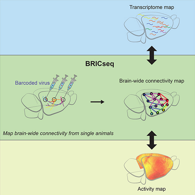
Comprehensive analysis of neuronal networks requires brain-wide measurement of connectivity, activity, and gene expression. Although high-throughput methods are available for mapping brain-wide activity and transcriptomes, comparable methods for mapping region-to-region connectivity remain slow and expensive because they require averaging across hundreds of brains. Here we describe BRICseq, which leverages DNA barcoding and sequencing to map connectivity from single individuals in a few weeks and at low cost. Applying BRICseq to the mouse neocortex, we find that region-to-region connectivity provides a simple bridge relating transcriptome to activity: The spatial expression patterns of a few genes predict region-to-region connectivity, and connectivity predicts activity correlations. We also exploited BRICseq to map the mutant BTBR mouse brain, which lacks a corpus callosum, and recapitulated its known connectopathies. BRICseq allows individual laboratories to compare how age, sex, environment, genetics and species affect neuronal wiring, and to integrate these with functional activity and gene expression.
ETOC:
BRICseq reproducibly maps brain-wide projections in individual mice and integrates connectivity to activity, genes and behaviors.
Graphical Abstract
Introduction
A central problem in neuroscience is to understand how activity arises from neural circuits, how these circuits arise from genes, and how they drive animal behaviors. A powerful approach to solving this problem is to integrate information from multiple experimental modalities. Over the last decade, high-throughput approaches have enabled both gene expression (Rodriques et al., 2019; Ståhl et al., 2016; Vickovic et al., 2019) and functional neural activity (Macé et al., 2011, 2018; Musall et al., 2019; Prevedel et al., 2014; Sofroniew et al., 2016; Stirman et al., 2016; Vanni and Murphy, 2014) to be assessed at whole-brain scale in individual subjects. Unfortunately, it remains challenging to assess long-range connectivity as rapidly and precisely. So the answers to fundamental questions of how connectivity is related to gene expression and neural activity, and how this relationship varies—in different species, genotypes, sexes and across developmental stages, as well as in animal models of neuropsychiatric disorders—remain elusive.
Historically, long-range connectivity maps were compiled manually from results generated by many individual laboratories, each using somewhat different approaches and methods, and each presenting data relating to one or a few brain areas of interest in idiosyncratic formats (Bota et al., 2015; Felleman and Van Essen, 1991; Scannell et al., 1995). Recent studies avoid the confounds inherent in inferring connectivity across techniques and laboratories by relying on a standardized set of tracing techniques (Bohland et al., 2009; Harris et al., 2019; Markov et al., 2014; Oh et al., 2014; Zingg et al., 2014). Even with improved methods, however, such maps remain expensive and labor-intensive to generate, so region-to-region connectivity has been studied only for a small number of model organisms, typically of a single sex, age and genetic background (Markov et al., 2014; Oh et al., 2014; Zingg et al., 2014).
The major bottleneck in conventional tracing methods arises from the difficulty in multiplexing tracing experiments. In classical connectivity mapping, a single tracer—for example, a virus encoding green fluorescent protein (GFP)—is injected into a “source” brain area (Harris et al., 2019; Oh et al., 2014; Zingg et al., 2014). The brain is then dissected and imaged, and any region in which GFP-labeled axonal projections are observed is a projection “target”. Fluorescence intensity at the target is interpreted as the strength of the projection. This procedure must be performed in a separate specimen for each source region of interest, since multiple injections within a single specimen would lead to ambiguity about which injection was the source of the observed fluorescence (Figure 1A). Although multi-color tract tracing methods can achieve some multiplexing by increasing the number of fluorophores (Abdeladim et al., 2019; Zingg et al., 2014), the increase in throughput is modest because only a small number of colors can be reliably distinguished. To obtain a region-to-region connectivity map, data must be pooled across hundreds of animals, and the associated labor and costs limit the ability to generate the region-to-region connectivity maps from distinct model systems.
Figure 1. Mapping brain-wide cortico-cortical projections with BRICseq.

A. In conventional fluorophore-based tracing, a separate brain is needed for each source area. B. In MAPseq, barcoded Sindbis virus is injected into a single source, and RNA barcodes from target areas of interest are extracted and sequenced. MAPseq multiplexes single neuron projections from a single source area. (BC = barcodes). C. In BRICseq, barcoded Sindbis is injected into multiple source areas. BRICseq multiplexes projections from multiple source areas, each at single neuron resolution. D. In the soma-max strategy for soma calling, the cubelet with the highest abundance of a particular barcode is posited to be the cubelet that contains the source of that barcode. E. Distributions of barcode abundance in source cubelets and target cubelets. F. Experimental validation of the soma-max strategy reveals an error rate <0.5%. G. BRICseq pipeline.
To achieve higher throughput at lower cost for mapping long-range, region-to-region connectivity in single animals, we sought to develop a method to enable multiplexing tracers for multiple source areas. Here we present BRICseq (BRain-wide Individual-animal Connectome sequencing), which leverages barcoding and high-throughput sequencing to multiplex tracing experiments from multiple source areas, and allows for mapping of brain-wide corticocortical connectivity from individual mice in a few weeks, and at low cost. Using the map of mouse neocortex connectivity derived from BRICseq, we find that region-to-region connectivity provides a simple bridge for understanding the relationship between gene expression and neuronal activity. Applying BRICseq to the mutant BTBR mouse strain, we recapitulated its known connectopathies. The ability of BRICseq to map brain-wide connectivity from single animals in individual laboratories will foster the comparative and integrative analysis of connectivity, neural activity, and gene expression across individuals, animal models of diseases, and novel model species.
Results
In what follows, we first describe the development of BRICseq, which allows mapping brain-wide projections from multiple sources in single animals. Next, we show that BRICseq is highly accurate and reproducible. We then show that BRICseq accurately predicts neural activity obtained by functional brain-wide calcium imaging in behaving mice, and that brain-wide gene expression predicts region-to-region connectivity. Finally, we show that BRICseq applied to the mutant BTBR mouse strain (which lacks a corpus callosum) can recapitulate its known connectopathies.
BRICseq allows for multiplexing connectivity tracing from multiple source areas
The multi-site mapping strategy we developed, BRICseq, builds on MAPseq (Kebschull et al., 2016a). In MAPseq (Figure 1B), multiplexed single neuron tracing from a single source was achieved by labeling individual neurons with easily distinguishable nucleotide sequences, or “barcodes”, which are expressed as mRNA and trafficked into axonal processes (Figure S1A). Because the number of nucleotide sequences, and therefore distinct barcodes, is effectively infinite—a short (30 base) random oligonucleotide has a potential diversity 430≈1018—MAPseq can be thought of as a kind of “infinite color Brainbow” (Livet et al., 2007). Brain regions representing potential projection targets are microdissected into “cubelets” and homogenized, and the barcodes within each cubelet are sequenced, permitting readout of single cell projection patterns. MAPseq has now been validated using several different methods, including single neuron reconstruction, in multiple brain circuits (Chen et al., 2019; Han et al., 2018; Kebschull et al., 2016a). In particular, single cells traced by MAPseq are statistically indistinguishable from traditional single cell reconstructions (Han et al., 2018), and MAPseq tracing efficiencies are comparable to that of traditional retrograde tracers (Chen et al., 2019; Kebschull et al., 2016a). The contribution of potential artifacts, including those due to degenerate labeling, fibers of passage, or non-uniform barcode transport, have been extensively quantified in previous work, and shown to be minimal (Chen et al., 2019; Han et al., 2018; Kebschull et al., 2016a).
MAPseq was originally developed to study projections from a single source. Conceptually, a straightforward generalization of MAPseq to determine the projections from many source areas in the same experiment would be to tag neurons with an additional area-specific barcode sequence—a “zipcode”—which could be used to identify the source (somatic origin) of each projection. In this approach, the overall strength of the projection from area 1 to area 2 would be determined by averaging the number of single neuron projections between those areas. In practice, however, such an approach would still be very labor intensive, because it would require the production, standardization and injection of hundreds of uniquely zipcoded batches of virus.
We therefore pursued a more convenient strategy, which requires only a single batch of virus (Figure 1C). We hypothesized that we could reliably determine the source of each projection using only sequencing, by exploiting the higher abundance of RNA barcodes in the soma-proximal compartments (including soma and proximal dendrites) compared with the axon terminals. According to this ‘soma-max’ strategy, the cubelet with the highest abundance of a given barcode of interest is assumed to be the source of the projection (Figure 1D). To validate this soma-max strategy, we injected two distinct viral barcode libraries, each identifiable by a known zipcode sequence, into two separate but densely connected cortical areas (primary motor area and secondary motor area). We dissected both injection sites, and sequenced the barcodes present in each (Figure 1E). Compared to the ground truth determined by the zipcode, the soma-max strategy correctly identified the soma location for 99.2±0.2% (mean±S.D.) of all cells (Figure 1F). These results indicate that the soma-max strategy would allow accurate reconstruction of connectivity even when only a single viral library is injected.
Mapping brain-wide corticocortical region-to-region connectome with BRICseq
We first applied BRICseq to determining the region-to-region connectivity of the cortex of the adult male C57BL/6J mouse, for which there exist reference data sets (Oh et al., 2014; Zingg et al., 2014). To do so, we tiled the entire right hemicortex of each mouse with barcoded virus by making over 100 penetrations (3–6 injections/penetration at different depths) in a grid pattern with 500 μm edge length (Figure S1B; Supplemental Table 1). Forty-four hours after viral injection, we cryosectioned the brain into 300 μm coronal slices, and used laser dissection to generate cortical (arc length ~ 1 mm) and subcortical cubelets (Figure 1G, Figure S1C,D). The locations of all cortical cubelets were registered to the Allen Reference Atlas (2011 version, Figure 1G, Supplemental Table 3) (Fürth et al., 2018; Sunkin et al., 2013). We then quantified the number of each barcode sequence in each cubelet by sequencing (Figure 1G, Figure S1D).
In six adult male C57BL/6J mice (BL6–1, BL6–2, BL6–3, BL6–4, BL6–5, and BL6–6) we mapped the connections from 98±11 (mean±S.D.) source cubelets to 246±17 target cubelets (225±10 cortical, 22±7 subcortical). All dissected cubelets were potential targets; source cubelets were defined as the subset of all cubelets containing barcoded somata. Although in principle the ‘soma-max’ strategy was able to correctly define the source cubelet for each barcode (Figure 1F), in practice we required the a barcode to have a count >250 in its source cubelet to further reduce errors (such as errors caused by re-used barcodes, see STAR Methods). With this criterion, from each source cubelet we obtained the sequences of several hundred somata (671±1.3×10³) located therein, as well of projections from several thousand (1.3×10³±2.3×10³) neurons with somata located elsewhere. The variation of the number of infected cells mainly resulted from various injection difficulties in different brain areas (e.g. lateral brain areas such as insular areas are more difficult to target than dorsal areas) as well as titer variations of different viral batches for different animals. We aggregated these single neuron data (Figure S2A-C) to calculate region-to-region axonal projection strengths (Figure 2A,B, Figure S3A, Supplemental Video, Supplemental Table 2). Thus the strength of the projection from source cubelet X to target cubelet Y was defined as the number of barcodes in target Y originating from somata in source region X divided by the number of somata in X. We also estimated a confidence bound on our estimate of the strength of each connection (Figure S2R,S; STAR Methods), by modeling two major error sources of false positives: PCR template switching (Figure S2D-G; STAR Methods) and re-used barcodes by multiple neurons (Figure S2H-N; STAR Methods). All self-self projection strengths were set to 0. In addition, we focused on mapping long-distance connections here by setting all the neighbor-projection strengths to 0, to avoid potential false positive local connectivity due to dendritic innervation of neighboring cubelets. Although in principle BRICseq data can be used to determine single neuron projection patterns, in practice sequencing depth and template sequencing precluded such an analysis for this dataset.
Figure 2. Brain-wide corticocortical projectome mapped by BRICseq and its validation.

A,B. Cubelet-to-cubelet connectivity of mouse BL6–1. In B, Each row is a source cubelet, and each column is a target cubelet. Cubelets are assigned to their primary brain area. FR, frontal areas; MO, motor areas; SS, somatosensory areas; VIS, visual areas; AUD, auditory areas; STR, striatum; TH, thalamus; AMY, amygdala; TEC, tectum; P/M/SC, pons/medulla/spinal cord; OB, olfactory bulb.
BRICseq is reproducible and accurate
To fulfill its potential as a high-throughput method for determining connectivity, BRICseq must be both reproducible and accurate. To assess reproducibility, we compared connection data resulting from different BRICseq experiments. We first developed a computational pre-processing method to correct for variable experimental yields and/or sequencing depths across individual experiments (Figure S2W,X; STAR Methods). We next compared pairs of C57BL/6J connection maps, and found that the reproducibility of BRICseq was high. Estimated connection strengths were similar between tested brains (r = 0.83±0.04, n = 15 pairs, Figure 3A,B, Figure S3C, STAR Methods, Supplemental Table 4). Differences between the measured connections across individuals arose from some unknown combination of technical and biological variability. Major sources of technical variability likely include differences in injections and in dissection borders. We minimized biological variability by comparing subjects of the same age, sex and genetic background, but since the actual degree of animal-to-animal variability in cortical connections is unknown, these results represent an upper bound on the technical variability of BRICseq.
Figure 3. Validation of BRICseq.

A. Reproducibility of brain area-to-brain area connection maps between two mice, BL6–1 and BL6–2. The unity line is in black. Blue bars show mean±S.D. B. The histogram of Pearson correlations between all pairs of C57BL/6J brains. C,D. Connectivity determined by BRICseq agrees with the Allen Connectome Atlas. C, An example comparison of PTLp between the Allen Atlas and BRICseq of mouse BL6–1. D, Comparison of the Allen Connectome with either the Allen Connectome or the whole network determined by BRICseq of mouse BL6–1. Connections strengths were quantified in log scale (connections lower than 10−7 were set to 10−7), and then z-scored. The unity line is in black.
To assess the accuracy of BRICseq, we compared our results to the Allen Connectivity Atlas (Supplemental Table 2 in Oh et al., 2014), which was generated using conventional fluorophore-based techniques. The relationship between the ~100 cortical BRICseq cubelets (defined by dissection) and cortical “areas” (defined by the Atlas) was not one-to-one: Each area typically spanned several cubelets, and each cubelet contributed to several areas. We therefore limited the comparison to the subset of cubelets that resided primarily (>70%) in a single source area. The agreement between BRICseq and the Allen Atlas was good (R = 0.60±0.11, n = 52 source brain areas in 6 animals; Figure 3C,D; Figure S3H-J); indeed, the agreement was comparable to inter-experiment variability within the Allen Atlas (R = 0.70±0.15, n = 12 source brain areas; Figure 3D). This confirms that potential MAPseq artifacts (from e.g. degenerate labeling, fibers of passage (Figure 2V), non-uniform barcode trafficking) are minimal in BRICseq, as expected from previous work (Chen et al., 2019; Han et al., 2018; Kebschull et al., 2016a), and thus that BRICseq is a reliable method mapping region-to-region connectivity.
Connectivity determined by BRICseq predicted neural activity during an auditory decision-making task
Every neuron in the cortex receives input from thousands of other neurons in other cortical and subcortical areas. Full knowledge of the detailed connections and activities of all the inputs would provide a foundation for the precise prediction of the activity of any given neuron (Bock et al., 2011; Kim et al., 2014; Seung and Sümbül, 2014; Takemura et al., 2013; Yan et al., 2017). However, BRICseq provides only region-to-region connectivity, a much lower dimensional measure. We therefore assessed whether BRICseq could predict neural activity.
We hypothesized that region-to-region anatomical connections would predict region-to-region “functional connectivity,” i.e. the statistical relationship between the neural activity in distinct brain regions (Friston, 2011). To measure functional connectivity, we performed cortex-wide wide-field calcium imaging in awake transgenic (Emx-Cre; Ai93; LSL-tTA) well-trained mice engaged in an auditory decision task (Figure 4A-C) (Musall et al., 2019). In these mice, the calcium indicator GCaMP6f is expressed in excitatory cortical neurons. After registering calcium signals into the cubelet reference frame, the activity of each cubelet was calculated as the mean activity over all its pixels. In principle, wide-field calcium signals reflect population neural activity pooled across somata, dendrites and axons in a given brain area. However, because most neuropil in any region is associated with somata and dendrites within that region, most of the calcium signal reflects locally generated activity rather than long-range inputs (Makino et al., 2017). Thus, here we interpret the calcium activity of each cubelet as the population activity of neurons residing in it.
Figure 4. BRICseq predicts functional connectivity.

A. BRICseq connectivity compared with cortex-wide Ca2+ imaging. B. The auditory decision making task. C. A single frame example of cortex-wide wide-field calcium imaging in a behaving animal. D. The activity traces of two example pairs of cubelets. c, connection strength (UMI/neuron); r, Pearson correlation. The shaded boxes represent duration of stimulation. The two vertical lines represent the time of trial initialization (left) and licking spout available (right). E. Activity correlation between pairs of cubelets (mouse mSM64 in day E2) vs. reciprocal connection strengths between them (BL6–1). The median line is in red. F. Similar in E, but the activity-connectivity correlation (x axis) was quantified for all pairs of imaging experiments and BRICseq experiments. G. Residual activity correlation vs residual reciprocal connection strengths after removing distance-dependent components.
Figure 4 shows the relationship between anatomical connectivity measured by BRICseq and functional connectivity measured by wide-field calcium imaging, considering only cubelets in the right hemisphere for analysis. We used activity correlation between pairs of cubelets as a measure of functional connectivity. Anatomical connectivity between cortical areas alone (note subcortical inputs to cortex were not included for analysis here) predicted functional connectivity remarkably well, as shown both in example pairs of cubelets and in the population level (Figure 4D-F, see more analyses in Figure S4A,D-H). As the distance between cubelets had a large effect on the connection strength (Figure S6F) and activity correlation, we further removed distance-dependent components, and found that the residual connection strengths and activity correlations showed weaker, but still significant correlations (Figure 4G, see more analyses in Figure S4B,E-H). Moreover, we performed the same analyses from the same animals in the early training stages (the first 4–6 days of training, when the task performance was at the chance level), and found similar relationship between neural activity and connectivity (Figure S4C). The agreement between these two very different measurements suggests that much of the ongoing activity in the cortex during the auditory decision task can be explained by surprisingly simple interactions between connected cortical areas.
Connectivity determined by BRICseq can be predicted by low-dimensional gene expression data
We next set out to test whether gene expression could be used to predict connectivity (Fakhry and Ji, 2015; Fornito et al., 2019). We hypothesized that even though the patterns of gene expression that established wiring during development might have vanished at the time point we were examining, correlates of those patterns might persist into adulthood. We thus applied mathematical methods to search for gene expression patterns in the adult that could be used to predict the strengths of region-to-region connections (Figure S5A).
We first calculated cubelet-to-brain area connectivity based on BRICseq data, and used principal components analysis (PCA) to identify connectivity motifs shared between the two brains. In this analysis, the interpretation of each PC is a subset of correlated projection targets. Interestingly, a small number of the principal components (PCs) captured most of the variance in the connectivity data (Figure 5A; Figure S5B,C). Indeed, the reconstruction of brain connectivity based on just the first 10 PCs of brain BL6–1 was strongly correlated with both brain BL6–1 (r=0.93) and brain BL6–2 (r=0.72). PCA can be thought of as a way of “de-noising” the brain connectivity, in the same way that low-pass filtering is a way of de-noising a periodic signal (exploiting the fact that sinusoids are the eigenvectors of a periodic signal). The motifs described by these first 10 PCs represent the components of the connectivity common to the two brains, and thus the components that could potentially be explained by gene expression data from an independent data set. We therefore used connectivity reconstructed by top 10 PCs for predicting analysis.
Figure 5. Gene expression patterns predict connectivity determined by BRICseq.

A. PCA-based reconstruction of connectivity, using PCs and coefficients obtained from mouse BL6–1. The correlation coefficient is plotted between the connectivity reconstructed from first n PCs and either mouse BL6–1 (red) or BL6–2 (green). B,C. The performance of linear regression models using selected gene predictors. The linear models were trained using a training set in BL6–1, and then tested using the remaining testing set in BL6–1 as well as in BL6–2. B. The Pearson correlation between observed and predicted connectivity increases with the number of predictor genes. Red, the performance in the testing set in BL6–1. Green, the performance in BL6–2. Black, the null performance with the gene expression data shuffled before feature selection and linear regression. Error bars in red and green represent S.E.M.; error bars in black represent 95% confidence intervals. C. The scatter plot of observed versus predicted connectivity, using 10 gene predictors. Red, the testing set in BL6–1. Green, BL6–2. D. The fitting coefficients of top 10 gene predictors for top 10 connectivity PCs.
We next sought to predict the region-to-region connectivity from the gene expression in each cubelet. We first registered Allen in situ hybridization data, which depict the expression patterns of ~20,000 genes in brains of male, 8 week-old, C57BL/6J mice (Lein et al., 2007), into the coordinates of BRICseq cubelets. We pre-filtered genes to only include high-quality expression data (genes with robust expression patterns in multiple assays, Supplemental Table 5), and then used a greedy feature selection algorithm to identify 25 genes most effective for predicting connectivity using a linear model (STAR Methods). Interestingly, prediction accuracy plateaued after only about 10 gene predictors to a high level (BL6–1 testing set, Pearson r = 0.72±0.04; BL6–2, Pearson r = 0.62±0.008; Figure 5B-D, Figure S5D,E). Because of the highly correlated nature of gene expression, the identities these predictive genes were not unique; other sets of predictive genes performed about as well, consistent with the idea that these genes represent signatures of the genetic programs that established wiring during development. To address the possible concern that the finding of the low-dimensional genetic program is due to low spatial resolution of BRICseq, we also performed similar analysis with Allen connectivity atlas with higher spatial resolution (Oh et al., 2014), and found similar trends (Figure S5F,G). The ability of even a small number of marker genes to predict wiring agreement suggests that a substantial fraction of region-to-region connectivity patterns arise from low-dimensional genetic programs.
BRICseq recapitulated known connectopathies in the BTBR mouse brain
A key advantage of BRICseq is that it allows for rapid and systematic comparison of brain connectivity between model systems. We applied BRICseq to compare the cortical connectome of C57BL/6J (Figure 2B) to that of two BTBR mice (BTBR-1 and BTBR-2), an inbred strain lacking the corpus callosum and displaying social deficits (Fenlon et al., 2015; McFarlane et al., 2008; Wahlsten et al., 2003) (Figure 6A; Figure S6A). Most strikingly and as expected, BRICseq revealed a nearly complete absence of commissural cortical connections (Figure 6B,C; Figure S6B). In the C57BL/6J, commissural connections constitute 37.9±4.6% of total connections, whereas in BTBR the percentage is 1.8±0.3% (Figure 6D; the few remaining nonzero commissural connections in BTBR were found exclusively in target cubelets close to the midline, and likely represented dissection error and contamination from the ipsilateral hemisphere, see Figure S6C). Thus, the known connectopathies of the BTBR strain are recapitulated using BRICseq.
Figure 6. Comparison of the BTBR and C57BL/6J cortical connectivity.

A. Bright field images of a C57BL/6J brain slice and a BTBR brain slice. Blue arrows indicate absence of the corpus callosum. B. Cubelet-to-cubelet connection matrix showing connection strengths in the BTBR mouse (BTBR-1). C. Quantification of contralateral connection strengths in C57BL/6J and BTBR. *, Mann-Whitney test, p < 10−30, n = 456 source cubelets from 6 C57BL/6J mice, n = 77 source cubelets from 2 BTBR mice. Error bars represent S.E.M. D. Nonzero connections in C57BL/6J (BL6–1) and BTBR (BTBR-1). Numbers inside the parentheses indicate total counts of possible connections. Numbers outside the parentheses indicate total counts of non-zero connections. E. Distributions of ipsilateral/contralateral corticocortical connection strengths in C57BL/6J (BL6–1) and BTBR (BTBR-1). *, p < 10−69, Kolmogorov-Smirnov test.
We next systematically compared the topological properties of the ipsilateral cortical networks of the C57BL/6J and BTBR mice in the cubelet coordinate system (Bullmore and Sporns, 2009). Network analyses of BRICseq-derived region-to-region connectivity differ from previous studies (Oh et al., 2014; Swanson et al., 2017; Zingg et al., 2014), as the natural coordinate frame is given by regularly spaced cubelets and all data were obtained from a single individual.
Consistent with previous reports (Oh et al., 2014), in the C57BL/6J, connection strengths were well fit by a log-normal distribution (Figure 6E, left; see more analyses in Figure S6D,E). The decay of connection strength with distance (Figure S6F) was fit with a double exponential (BL6–1: scale parameter β1= 0.32±0.13 mm, β2= 3.96±3.25 mm, mean±95% confidence intervals), and connection probability (Figure S6F) with a single exponential (BL6–1: β= 1.42±0.23 mm, mean±95% confidence interval). Both the input correlations and output correlations between pairs of cubelets showed positively biased distributions (Figure S6G), and decayed with distance (Figure S6H). Interestingly, the distribution of ipsilateral connection strengths in the BTBR was similarly fit by a log-normal distribution (Figure 6E, right), and the inferred ipsilateral area-to-area connections were not grossly disrupted (Figure S6I-L).
We next analyzed the topological properties of the ipsilateral cortical networks. By decomposing the network into small motifs containing 2 or 3 cubelets, and quantitatively comparing the abundance of these motifs to randomly generated networks, we found that in the C57BL/6J, the fraction of 2-cubelet motif with a reciprocally connected pair was greater than the null model, and densely connected 3-cubelet motifs were also significantly overrepresented (Figure 7A,B, Figure S7A,B,E). Interestingly, the distribution of 3-cubelet motifs was strikingly similar to statistics of connections among single neurons in the rat visual cortex (Song et al., 2005), suggesting that a common rule might govern the organization of neural circuits at both microscale (inter-neuronal) and mesoscale (inter-regional) levels. Furthermore, four network modules—regions of the brain within which connections are dense, and which may reflect functional units—were revealed by connection-based clustering of cubelets in the C57BL/6J (Figure 7C,D, Figure S7G-K). These modules were not only similar to previously described connectional networks (Harris et al., 2019; Zingg et al., 2014), but also roughly matched the cytoarchitectonic map: approximately module 1 belonged to visual-auditory areas, modules 2 and 3 belonged to somatosensory/motor areas, and module 4 belonged to the anterior cingulate/retrosplenial areas. Moreover, modules 2 and 3 were not clustered according to the hierarchy in the Allen atlas (where the somatosensory and somatomotor areas are two modules in the highest hierarchy), but more reflected the represented body parts (roughly, module 2 corresponded to somatosensory and somatomotor areas assosciated with limbs, trunk and whiskers, and module 3 corresponeded to areas associated with mouth and nose), and showed similar patterns as revealed by functional imaging (Figure 5 in Vanni et al., 2017). Similar results were found in the BTBR (Figure S7C,D,F,L-N), suggesting that these high-order topological properties were largely maintained in the BTBR strain. Thus, although the commissural corticocortical connections are completely missing, the ipsilateral network remained largely intact in the BTBR mouse (Figure S6K,L). The failure to uncover differences, combined with the high sensitivity of BRICseq, provide a lower bound on the differences between BTBR and BL6 ipsilateral cortical networks.
Figure 7. Topological properties of the ipsilateral cortical network.

A,B. Abundance of 2-node and 3-node motifs in cortical network in C57BL/6J (BL6–1) compared to randomly generated networks. *, p < 0.001. C, Sorted cubelet-to-cubelet connection matrix based on modules in BL6–1. D. Connection-based modules in C57BL/6J (BL6–1). The same colors denote the same modules in C and D. The outlines of gross brain areas defined in Allen atlas are overlaid on top of D. The names of cortical areas based on the Allen atlas are shown in Figure S7O.
Discussion
This study describes BRICseq, a high-throughput and low-cost method which exploits sequencing of nucleic acid barcodes for determining region-to-region connectivity in individual animals. BRICseq of the neocortex of the C57BL/6J mouse revealed that region-to-region gene expression, connectivity and activity are related in a simple fashion: Spatial variations in as few as ten genes predict connectivity, and this connectivity in turn predicts correlations in neuronal activity. BRICseq of the BTBR mouse strain recapitulated the known deficits of commissural corticocortical connections. By virtue of its relatively low cost and high-throughput, BRICseq enables individual laboratories to study how age, sex, environment, genetics, and species affect neuronal wiring, how these are disrupted in animal models of disease or modified after manipulations, and to integrate these with functional activity, gene expression and behavioral phenotypes in individual animals.
Comparison with other methods
BRICseq is high throughput and low cost by comparison with current methods for obtaining a comparable data set. Conceptually, BRICseq is closest to conventional fluorophore-based tracing techniques (Oh et al., 2014; Zingg et al., 2014). However, whereas conventional fluorophore-based approaches require pooling across hundreds of brains to map brain-wide connectivity, BRICseq multiplexes injections and is thereby able to map connectivity from individual subjects. This multiplexing reduces costs, labor, and animal-to-animal variability. Currently it takes less than 4 weeks for a single person to perform one BRICseq experiment at the total cost of less than $10,000 (including the sequencing cost). The ability to generate maps from single subjects eliminates the need to register anatomical coordinate systems across animals, which increases reproducibility and accuracy. Reducing the number of subjects also leads to a substantial decrease in the total cost, both in terms of money and labor. The reduction in the number of subjects is particularly appealing for the study of non-human primates (Izpisua Belmonte et al., 2015), as well as of relatively new model systems for which connectivity maps are not yet available or individual subjects are particularly valuable, such as the Alston’s singing mouse (Banerjee et al., 2019; Okobi et al., 2019) and peromyscus (Bedford and Hoekstra, 2015; Metz et al., 2017; Weber et al., 2013).
Connectivity can also be mapped using diffusion tractography imaging (DTI), which uses 3D tracing of water diffusion pathways measured by MRI to infer the orientation of white matter tracts in the brain (Calabrese et al., 2015). Because DTI is rapid and non-invasive, it is widely used in the study of human brain connectivity. However, conventional DTI has low spatial resolution and low signal-to-noise ratio, and has difficulty resolving subvoxel fiber complexity, so it has been much less useful in the study of small animal connectivity. Moreover, DTI requires access to specialized small animal MRI scanners, which remain relatively uncommon. Thus despite recent advances in small animal DTI, this approach has not become widely adopted.
BRICseq differs from conventional fluorophore tracing in that the spatial resolution is determined at the time of dissection (for sources and targets), rather than as with fluorophore tracing at the time of injection (for sources) and imaging (for targets). In the present study, we dissected rather large cubelets, and the cubelet size we chose currently may limit the mapping of small brain regions, particularly when BRICseq is applied to subcortical nuclei in the future. However, laser capture microdissection permits much smaller cubelets, even approaching single neuron resolution, allowing BRICseq experimenters to dynamically adjust the dissection size according to experiment needs, or even perform nucleus-specific dissection following online registration of brain slices. Moreover, spatial transcriptomic methods (Rodriques et al., 2019; Ståhl et al., 2016; Vickovic et al., 2019), including in situ sequencing (Chen et al., 2019), raise the possibility of achieving single cell and indeed single axon or even synaptic resolution.
The sensitivity of BRICseq depends on a number of factors, including the number of infected cells per cubelet, the false positive error rate, and the sequencing depth. Although as shown in the current manuscript, corticocortical connectivity maps determined by the current BRICseq protocol are overall highly reproducible and accurate compared to Allen connectivity atlas, it could be further improved to detect and compare relatively weak connections or even at single neuron resolution. For instance, the viral injection protocol can be further optimized to make the number of infected cells per cubelet - and thus the sensitivity (Figure S2U) - more uniform, across all the cubelets. In addition, the development of non-invasive viral delivery techniques may also provide alternative approaches for efficient brain-wide barcoding of neurons for BRICseq (Chan et al., 2017; Wang et al., 2019). To further reduce the template switching error rate (Figure S2D-G), we could perform PCR separately for each cubelet, or implement droplet PCR (Hindson et al., 2011). To reduce the re-used barcode rate (Figure S2H-N), we are able to make viral libraries with much higher barcode diversity (indeed we have already attempted to make one and used it in BL6–6 and BTBR-2). Moreover, we envision the rapid progress of high-throughput DNA sequencing methods, allowing for much higher sequencing depth and lower costs in the near future. We expect that with further improvement, BRICseq will enable us to map brain-wide connectivity with much higher throughput and sensitivity; moreover, because the technical variability of BRICseq mainly results from the variability of viral injection, cubelet dissection, sequencing depth, and false positive errors, such improvement will also allow for further reduction of BRICseq variability.
Compared with conventional fluorophore-based approaches, currently BRICseq is not able to map connectivity in a presynaptic cell type-specific manner. Although the expression of RNA virus Sindbis cannot be controlled by DNA recombinase Cre or Flp, it is possible to pseudotype Sindbis by replacing its glycoprotein to restrict its tropism to a specific cell type, achieving presynaptic cell-specificity in a way similar to the pseudotyped rabies (Wickersham et al., 2007). In addition, the development of in situ sequencing (Chen et al., 2019; Lee et al., 2015; Wang et al., 2018) may also allow for brain-wide assessment of connection and gene simultaneously, relating transcriptome to connectome at even single synaptic resolution.
Simple relationship among gene expression, connectivity and activity
At one level, our finding that there is a simple relationship (Figures 4,5) among gene expression, connectivity and functional activity may not seem unexpected. The genome encodes the developmental rules for wiring up a brain—rules that are implemented in part by spatial patterns of gene expression—and this wiring in turn provides the scaffolding for resting state or “default” neuronal activity (Buckner et al., 2008). So the fact that gene expression, connectivity and functional activity are related is a direct consequence of development and brain architecture.
However, what is surprising is not that a relation exists among gene expression, connectivity and functional activity, but that this relationship is simple. Wiring could depend in complex and nearly indecipherable ways on dozens or even thousands of gene-gene interactions. Thus the fact that region-to-region connectivity of the neocortex could be predicted by the spatial expression pattern of just a small number (~10) of genes raises the possibility that low-dimensional genetic programs determine the interregional wiring of the cortex. However, despite the predictive power of these 10 genes (Figure 5), there is no reason to expect that these predictive genes were causal in establishing wiring; they might merely be correlated with the causal genes. To establish the causal effect of genes on connectivity will likely require experiments in which gene expression is perturbed. Fortunately, BRICseq is sufficiently high-throughput that such an experimental program might not be prohibitively expensive.
We also observed that the corticocortical connectivity between two regions could predict correlations in cortical activity between them (Figure 4). Interestingly, a previous study (Honey et al., 2009) in humans found only a weak relationship between structural connectivity (assessed by DTI) and functional connectivity (inferred from resting state correlations). Whether these different results arise from methodological considerations (e.g. widefield calcium imaging and BRICseq vs. fMRI and DTI; task engagement vs. resting state), or whether they reflect fundamental differences between mice and humans, remains to be determined.
In the present experiments, gene expression, connectivity and activity were all assessed separately, in different individuals. The data from these different experiments were then aligned to a shared coordinate system. However, because the techniques used in these experiments—widefield imaging, RNAseq of endogenous transcripts and sequencing of barcodes—are mutually compatible, it is feasible to combine them all in single individuals. Not only would this eliminate variability arising from combining data across individuals, it would also allow both connectivity and gene expression to be determined in the same coordinate system. Because the alignment to a common coordinate system represents a significant source of animal-to-animal variability, we expect that the simplicity of the relationships reported here represent a lower bound on the actual variability.
BRICseq in the era of comparative connectomics
Growing evidence suggests that disruption of interregional connectivity leads to a variety of neuropsychiatric disorders, such as autism and schizophrenia (Geschwind and Levitt, 2007; Kubicki et al., 2007). Deciphering the circuit mechanisms underlying brain disorders requires systematic characterization of connectopathies, how they disrupt brain activity, and how they result from genetic mutations. Investigation of diverse animal models can reveal the neural mechanisms underlying species-specific behaviors, and provide a path toward discovering general brain principles (Yartsev, 2017). However, brain-wide interregional connectivity in animal models of diseases and new species remain largely unavailable, in part because of the lack of a high-throughput, inexpensive and accurate technique. Thus, we expect that BRICseq, combined with other brain-wide individual-animal imaging or RNAseq techniques, will facilitate the creation of a systematic foundation for studying circuits in diverse animal models, opening up the possibility of a new era of quantitative comparative connectomics.
STAR Methods
Resource availability
Lead contact
Further information and requests for resources and reagents should be directed to and will be fulfilled by the Lead Contact, Anthony M Zador (zador@cshl.edu).
Materials availability
The genomic construct and the helper construct for Sindbis virus production are available from Addgene under accessions 73074 and 72309. Sindbis virus and BRICseq services are available from the MAPseq core (hzhan@cshl.edu) in the Cold Spring Harbor Laboratory upon reasonable request.
Data and code availability
All sequencing datasets are publicly available under SRA accession codes SRA: PRJNA541990. Further information and requests for data and code should be directed to and will be fulfilled by the Lead Contact.
Experimental model and subject details
Animal models used in the paper include: (model organism: name used in paper: genotype) Mouse: C57BL/6J: C57BL/6J; Mouse: BTBR: BTBR T+ Itpr3tf/J; Mouse: Emx-Cre: Emx1tm1(cre)Krj/J; Mouse: Ai93: Igs7tm93.1(tetO-GCaMP6f)Hze/J; Mouse: LSL-tTA: Gt(ROSA)26Sortm1(tTA)Roos/J; Mouse: CamKII-tTA: CBA-Tg(Camk2a-tTA)1Mmay/J.
Animal procedures were approved by the Cold Spring Harbor Laboratory Animal Care and Use Committee and carried out in accordance with National Institutes of Health standards. For BRICseq, experimental subjects were 8-week-old male C57BL/6J mice or BTBR T+ Itpr3tf/J mice from the Jackson Laboratory. For functional imaging, triple transgenic mice Emx-Cre; Ai93; LSL-tTA were generated. A small fraction of mice used for functional imaging also harbored a CamKII-tTA allele to enhance the expression of GCaMP6f.
Method details
Sindbis virus barcode libraries
The Sindbis virus used in BRICseq was made as described previously (Kebschull et al., 2016b, 2016a). Briefly, based on a dual promoter pSinEGdsp construct, we inserted MAPP-nλ after the first subgenomic promoter, and GFP-BC(barcode)-4×boxB after the second subgenomic promoter. Sequences (5’)AAG TAA ACG CGT AAT GAT ACG GCG ACC ACC GAG ATC TAC ACT CTT TCC CTA CAC GAC GCT CTT CCG ATC TNN NNN NNN NNN NNN NNN NNN NNN NNN NNN NNN GTA CTG CGG CCG CTA CCT A(3’) were inserted between MluI and NotI sites which were between GFP and 4×boxB. In barcode library 1, the 32-nt BC ended with 2 purines, while in barcode library 2, the 32-nt BC ended with 2 pyrimidines. Sindbis virus was produced using the DH-BB(5’SIN;TE12ORF) helper plasmid (Kebschull et al., 2016b). One batch of library 1 viruses and two batches of library 2 viruses were used in the project. The viral barcode library diversity was determined by Illumina sequencing. ~ 2 × 10⁶ barcodes were sequenced in the viral library 1, ~ 8 × 10⁶ barcodes were sequenced in the first viral library 2 (used in BL6–1, BL6–2, BL6–3, BL6–4, BL6–5 BTBR-1, soma calling strategy validation experiment and template switching volume test experiment), and > 2.7 × 10⁸ barcodes were sequenced in the second viral library 2 (used in BL6–6 and BTBR-2). Significantly higher barcode diversity was achieved in the seconds viral library 2 by removing unligated DNA after barcode insertion between MluI and NotI using Plasmid Safe DNAse (Epicentre) according to manufacture’s instructions. This dramatically increased bacterial electroporation efficiencies and thus plasmid library diversity. In addition, virus was produced in Corning CELLStacks to increase the number of virus producing cells 30-fold over the first virus library 2, easing this second diversity bottleneck.
Injections
For BRICseq, Sindbis virus of barcode library 2 was injected into the right cortical hemispheres of experimental animals. Anesthesia was initially induced with isoflurane (4% mixed with oxygen, 0.5 L/min). Meloxican (2 mg/kg), dexamethasone (1 mg/kg) and baytril (10 mg/kg) were then administered subcutanesouly. For Sindbis injections, the whole skull above the right cortical hemisphere was removed. More than 100 injection pipette penetrations were made to cover the entire exposed brain, each spaced by 0.5 mm, both in the AP axis and ML axis. Nanoject III (Drummond Scientific) was used to inject Sindbis virus (~2 × 10¹⁰ GC/mL), at 3–4 depths per penetration site (Supplemental Table 1). At each penetration site and depth, 23 nL virus was injected. The full injection surgery required about 8 hours, and constant isoflurane (1% mixed with oxygen, 0.5 L/min) was administered to maintain anesthesia. After injection, sterile Kwik-Cast (World Precision Instruments) was gently applied to cover the exposed brain region, and the skin was closed with sutures. Meloxican (2 mg/kg), dexamethasone (1 mg/kg) and baytril (10 mg/kg) were then routinely administered to animals subcutaneously every 12 hours post surgery, and animal condition was inspected every 6 – 12 hours. Similarly, we injected Sindbis virus of barcode library 1 into control animals. In control animals, instead of injecting the virus into the whole right cortex, we only made ~6 penetrations covering a small cortical area.
For control experiments testing the soma calling strategy (Figure 1E,F, Figure S2T), the same BRICseq protocol was followed, but Sindbis virus of barcode library 1 was injected into the secondary motor areas, and Sindbis virus of barcode library 2 into the primary motor areas.
For control experiments testing template switches (Figure S2D-F), we followed the BRICseq protocol above, but injected Sindbis virus of barcode library 2 into two separate animals.
For AAV CAG-tdTomato tracing experiments (Figure S6A), we used coordinates AP = −4 mm, ML = 0.5 mm, 1 mm and 1.5 mm, DV = 0.25 mm and 0.5 mm for retrosplenial cortex in C57BL/6J and coordinates AP = −4 mm, ML = 0.75 mm, 1 mm and 1.5 mm, DV = 0.25 mm and 0.5 mm for retrosplenial in BTBR. In BTBR, as two hemispheres began to separate at AP = −4 mm and there was no cerebral cortex at ML = 0.5 mm, we used ML = 0.75 mm instead. In each coordinate, 20 nL of AAV1 CAG-tdTomato AAV (2×10¹³ GC/mL Penn Vector Core) was injected.
Cryosectioning and laser microdissection (LMD)
In BRICseq, 44 hours after Sindbis viral injection, the brain was harvested and fresh frozen at −80 °C. Olfactory bulbs and rostral spinal cord/caudal medulla were cut from the brain and collected separately. We then cut 300 μm coronal sections using a Leica CM 3050S cryostat at −12 °C chamber temperature and −10 °C object temperature. Each slice was cut with a fresh part of a blade, and the platform and brushes were carefully cleaned between slices. Each slice was immediately mounted onto a steel-framed PEN (polyethylene naphthalate)-membrane slide (Leica). After mounting on the slide, the slice was fixed in 75% ethanol at 4 °C for 3 min, washed in Milli-Q water (Millipore) briefly, stained in 0.5% toluidine blue (Sigma-Aldrich, MO) Milli-Q solution at room temperature for 30 sec, washed in Milli-Q water at room temperature for 3 times (15 sec each time), and fixed again in 75% ethanol at room temperature twice (2 min each time). The slide was then left in a vacuum desiccator for 30 min. Next, another fresh frame slide was used to sandwich the brain slice, and the two slides tightly taped to prevent the slice from falling. The sandwiched slice was stored in the vacuum desiccator at room temperature until LMD. If LMD was performed more than 1 week after cryosectioning, the sandwiched slices were stored at −80 °C in a desiccated container.
Cubelet dissection was performed with Leica LMD 7000. During LMD, cortical cubelets with ~1 mm arc length were dissected from each coronal slice, from the surface to the deepest layer above the white matter. Orbitofrontal cortical cubelets (in rostral slices), anterior cingulate cortical cubelets, and retrosplenial cortical cubelets were also collected separately. For subcortical areas including striatum, thalamus, amygdala, tectum and pons/medulla, tissue belonging to each brain area was pooled every 1–3 consecutive slices. About 12~21 cubelets were also collected from injection sites and contralateral homotopic areas of the injection sites in the barcode library 1 control animal, and 2 cortical cubelets in the uninjected control animal. Pictures were taken before and after every cubelet was dissected. After dissecting every 4 cubelets, we transferred them into homogenizing tubes with homogenizing beads, and added 100 μL lysis solution (RNAqueous-Micro Total RNA Isolation Kit, Thermo Fisher) into each cubelet. The collected tissues were stored temporally on dry ice and then at −80 °C.
Sequencing library preparation
After LMD, each cubelet was homogenized in lysis solution with a tissue lyser (Qiagen) at 20 Hz for 6 min. Then we extracted RNA molecules from each cubelet with RNAqueous-Micro Total RNA Isolation Kit (Thermo Fisher). We did not treat products with DNase i as DNA did not influence following experiments. The final product was eluted in 20 μL elution solution.
After RNA extraction, we performed reverse transcription (RT) with barcoded RT primers using SuperScript IV (Thermo Fisher). Barcoded RT primers were in the form of (5’)CTT GGC ACC CGA GAA TTC CAX XXX XXX XXX XXZ ZZZ ZZZ ZTG TAC AGC TAG CGG TGG TCG(3’) (for BL6–1, BL6–2, BTBR-1 and BTBR-2), or (5’)CTT GGC ACC CGA GAA TTC CAX XXX XXX XXX XXX XZZ ZZZ ZZZ ZZZ ZZZ ZZT GTA CAG CTA GCG GTG GTC G(3’) (for BL6–3, BL6–4, BL6–5 and BL6–6), where Z8/Z16 is one of 288 CSIs (cubelet-specific identifiers) and X12/X14 is the UMI (unique molecular identifier). 1 μL of 1 × 10⁻⁹ μg/μL spike-in RNAs were also added. The sequence of spike-in RNAs were (5’)GUC AUG AUC AUA AUA CGA CUC ACU AUA GGG GAC GAG CUG UAC AAG UAA ACG CGU AAU GAU ACG GCG ACC ACC GAG AUC UAC ACU CUU UCC CUA CAC GAC GCU CUU CCG AUC UNN NNN NNN NNN NNN NNN NNN NNN NAU CAG UCA UCG GAG CGG CCG CUA CCU AAU UGC CGU CGU GAG GUA CGA CCA CCG CUA GCU GUA CA(3’).
We then cleaned up RT products with 1.8×SPRI select beads (Beckman Coulter), synthesized double-stranded cDNA with previously described methods (Morris et al., 2011), cleaned up 2nd strand synthesis products again with 1.8× SPRI select beads, and treated the eluted ds cDNA with Exonuclease i (New England Biolabs) (incubated the mix at 37°C for 1 hr and inactivated the enzyme at 80°C for 20 min). As cDNA molecules from different cubelets were already CSI-barcoded after RT, we pooled every 12 RT products for 1st bead purification and 2nd strand synthesis, and pooled all the products for 2nd bead purification and Exonuclease i treatment.
We next amplified the cDNA library by nested PCR using primers (5’)GGA CGA GCT G(3’) and (5’) CAA GCA GAA GAC GGC ATA CGA GAT CGT GAT GTG ACT GGA GTT CCT TGG CAC CCG AGA ATT CCA(3’) for the first PCR and primers (5’)AAT GAT ACG GCG ACC ACC GA(3’) and (5’) CAA GCA GAA GAC GGC ATA CGA(3’) for the second PCR in Accuprime Pfx Supermix (Thermo Fisher). First PCR was performed for 5 cycles in 720 μL; after Exonuclease i treatment (incubated the mix at 37°C for 30 min and inactivated the enzyme at 80°C for 20 min), ¼ of the first PCR products were used for second PCR. Second PCR was performed for 5–10 cycles in 12 mL. Standard Accuprime protocol was used for PCR except that the extension time in each cycle was set to 2 min to reduce incomplete elongation and template switches.
Nested PCR products were then purified and eluted in 600 μL with a Wizard SV Gel and PCR Clean-Up System (Promega), and further concentrated with Ampure XP beads (Beckman Coulter) in 25 μL Milli-Q H2O. After running in a 2% agarose gel, the 230 bp band was cut out and cleaned up with the Qiagen MinElute Gel Extraction Kit (Qiagen). We sequenced the library on an Illumina Nextseq500 high output run at paired end 36 using the SBS3T sequencing primer for paired end 1 and the Illumina small RNA sequencing primer 2 for paired end 2.
Most of the molecular experiments were performed according to the reagent manufacturer’s protocol unless otherwise stated.
Sequencing
We sequenced the pooled libraries prepared as above on an Illumina Nextseq500 high output run at paired end 36 using the SBS3T sequencing primer for paired end 1 and the Illumina small RNA sequencing primer 2 for paired end 2.
Confocal imaging
In AAV tracing experiments, brains were harvested 14 days after viral injection, fixed in 4% paraformaldehyde, washed in phosphate-buffered saline, and cut into 100 μm slices with a vibrotome (LeicaVT1000S, Leica). Slices were then mounted onto slides in Fluoroshield (Sigma-Aldrich), and imaged in a Laser Scanning Microscope 710 system (Leica).
Wide-field calcium imaging
Wide-field calcium imaging experiments in Figure 4 and Figure S4 are as described in (Musall et al., 2019). All surgeries were performed under 1–2 % isoflurane in oxygen anesthesia. After induction of anesthesia, 1.2 mg/kg of meloxicam was injected subcutaneously and lidocaine ointment was topically applied to the skin. After making a medial incision, the skin was pushed to the side and fixed in position with tissue adhesive (Vetbond, 3M). We then created an outer wall using dental cement (Ortho-Jet, Lang Dental) while leaving as much of the skull exposed as possible, then a circular headbar was attached to the dental cement. After carefully cleaning the exposed skull we applied a layer of cyanoacrylate (Zap-A-Gap CA+, Pacer technology) to clear the bone. After the cyanoacrylate was cured, cortical blood vessels were clearly visible.
Widefield imaging was done using an inverted tandem-lens macroscope in combination with an sCMOS camera (Edge 5.5, PCO) running at 60 fps. The top lens had a focal length of 105 mm (DC-Nikkor, Nikon) and the bottom lens 85 mm (85M-S, Rokinon), resulting in a magnification of 1.24×. The total field of view was 12.4 × 10.5 mm and the spatial resolution was ~20μm/pixel. To capture GCaMP fluorescence, a 500 nm long-pass filter was placed in front of the camera. Excitation light was coupled in using a 495 nm long-pass dichroic mirror, placed between the two macro lenses. The excitation light was generated by a collimated blue LED (470 nm, M470L3, Thorlabs) and a collimated violet LED (405 nm, M405L3, Thorlabs) that were coupled into the same excitation path using a dichroic mirror (#87–063, Edmund optics). From frame to frame, we alternated between the two LEDs, resulting in one set of frames with blue and the other with violet excitation at 30 fps each. Excitation of GCaMP at 405 nm results in non-calcium dependent fluorescence, and we could therefore isolate the true calcium-dependent signal by rescaling and subtracting frames with violet illumination from the preceding frames with blue illumination. All subsequent analysis was based on this differential signal at 30 fps.
Behavior task
For Figure 4 and Figure S4, the behavior has previously been described in Musall et al., 2019. Briefly, four mice were trained on a delayed 2-alternative forced-choice (2AFC), spatial discrimination task. Mice initiated trials by touching two handles. After one second of holding the handles, mice were presented with a sequence of auditory clicks for a total of up to 1.5 s. In each trial, click sequences were presented either on the left or right side of the animal. A 1 s delay was then imposed, after which servo motors moved two lick spouts into close proximity of the animal’s mouth. Licks to the spout corresponding to the stimulus presentation side were rewarded with water. After one spout was contacted, the opposite spout was moved out of reach to force the animal to commit to its initial decision. Animals were trained over the course of approximately 30 days and reached stable detection performance levels of 80% or higher.
Quantification and statistical analysis
LMD (laser microdissection) Image processing
Wholebrain toolbox (by Daniel Fürth, http://www.wholebrainsoftware.org) was used to register Toluidine Blue-stained coronal slices into Allen Reference Atlas semi-automatically. Using Matlab, we determined the coordinates of each cubelet by processing pictures taken before and after each cubelet was dissected. Combining image registration results and cubelet coordinates, we mapped each cubelet into one or multiple brain areas.
BRICseq data analysis
In what follows, we will describe methods to determine brain-wide connectivity maps from BRICseq data. For clarity of methodological details, we define the following terms first. 1) Barcode: a barcode is a unique 32nt sequence delivered by the Sindbis virus. One barcode theoretically corresponds to a neuron. 2) Molecule: here a molecule is defined as a unique BC-CSI-UMI (32nt + 8nt + 12nt) sequence. A molecule should correspond to a single RT product. Due to barcode amplification in a neuron, one barcode has multiple molecules. 3) Molecule copy: a molecule copy is defined as a final product after PCR. A large number of molecule copies are generated from one molecule during PCR. 4) Read: reads are the sequencing product. PCR products are sent for high-throughput sequencing, so reads can be considered as undersampled molecule copies.
Processing of raw sequencing data
Raw Illumina sequencing results consisted of two .fastq files: 32-nt BC sequences were in paired end 1, and 12-nt UMI and 8-nt CSI sequences (BL6–1, BL6–2, BTBR-1, BTBR2) or 14-nt UMI and 16-nt CSI sequences (BL6–3, BL6–4, BL6–5, BL6–6) were in paired end 2. The full BC-UMI-CSI sequences were merged and then de-multiplexed based on CSIs (cubelets). All the sequences with ambiguous bases (shown as N in the sequencing results) were removed. We then collapsed all the identical reads. Based on the sequencing depth (Kebschull and Zador, 2015), we set the read threshold as 0 (including all reads) for BL6–1, BL6–2, BL6–3, BL6–4, BL6–6 and BTBR-1, and set the read threshold as 1 (only include molecules with >1 reads) for BL6–5 and BTBR-2. Unique sequences were next sorted into barcode library 1 (BC ended with 2 purines), barcode library 2 (BC ended with 2 pyrimidines), and spike-in (BC ended with ATCAGTCA). We then counted the number of unique UMIs for each BC-CSI, which represented the molecule count of a given barcode in a given cubelet.
Substitution error correction
Base substitution is one of the major error sources. As the theoretical diversity of a random barcode of N30YY or N30RR is 430×22 ≈ 1018, an error barcode due to substitution should be very similar to one of the real barcodes, while any two real barcodes should be very different. To correct substitution errors, we first found all the barcode pairs with up to 3 mismatches using the short read aligner bowtie (http://bowtie-bio.sourceforge.net/index.shtml) (Langmead et al., 2009). We next collapsed all the barcodes into a large number of clusters, such that for any barcode (BC1) in a given cluster, there existed another barcode (BC2) in the same cluster with less than 3 mismatches. As a simple algorithm, theoretically it could cause very different barcodes to be collapsed into the same cluster; however, this did not happen in the real scenario due to the high hamming distances between used barcodes (Kebschull and Zador, 2015). The barcode with the highest UMI counts in each cluster was used to represent the cluster, and the summed UMI count of all the barcodes in the cluster was calculated as the corrected UMI count of the barcode. After substitution correction, we generated a barcode-cubelet matrix, where each element represented the molecule count of a given barcode in a given cubelet after collapsing.
Reconstruction of single cell projections
With following steps, we determined each cell’s location and its projection pattern.
Step 1: viral abundance thresholding. For viral library 2, batch 1 experiments (BL6–1, BL6–2, BL6–3, BL6–4, BL6–5, BTBR-1), as the barcode counts in the viral library were not perfectly uniform (Figure S2J), to reduce re-used barcode errors, barcodes whose counts were greater than 5 in the viral library sequencing result were excluded for analysis in the barcode-cubelet matrix (for details on how the viral abundance threshold affects re-used barcodes, please see section ‘correction of re-used barcodes’). For viral library 2, batch 2 experiments (BL6–6, BTBR-2), due to the high barcode diversity, no viral abundance threshold was used.
Step 2: UMI thresholding. To remove noises, we set all the no-greater-than-1 (UMI threshold) elements in the matrix to 0.
Step 3: soma/axon thresholding. After barcode abundance thresholding and UMI thresholding, we determined the soma location of each barcode using the ‘soma-max’ strategy. To exclude local dendritic innervations, for each barcode, the UMI counts of all the cubelets neighboring to the soma cubelet were set to 0. Firstmax and secondmax were then calculated as the highest and second highest UMI counts for each barcode. We chose soma threshold to be 250 and axon threshold to be 20, and only analyzed barcodes whose firstmax was greater than soma threshold and secondmax was between UMI threshold and axon threshold. The purpose of soma/axon thresholding was to correctly identify source cubelets for each barcode, and to reduce the number of re-used barcodes. For details on how the thresholds affect the ratio of re-used barcodes, please see section ‘correction of re-used barcodes’.
Step 4: filter right cortical neurons. We remove the barcodes whose somas did not reside in the right cortical hemisphere. Cells not in the right cortex were extremely rare, and they were likely due to virus spread.
Calculating bulk projections and confidence bounds
To calculate bulk projection patterns, we pooled all the projection cells that resided in the same cubelets together, and calculated their average projection patterns. As some error sources including PCR template switching and re-used barcodes contributed to false positive connections, we also estimated false positive connection strengths, subtracted them from raw connection strengths, and calculated p values for each connection. The details are as follow:
Step 1. Correct raw connection strengths: The raw projection strength from a source cubelet to a target cubelet was defined as the total count of UMIs in the target cubelet from all the neurons residing in the source cubelet divided by total number of projection neurons in the source cubelet. Considering the projection from cubelet i to cubelet k, let N(i) denote number of projection neurons in cubelet i and UMI(i, j, k) denote the UMI count in cubelet k from jth neuron in cubelet i, then the UMI count in cubelet k from an average neuron in cubelet i, UMI(i,*, k) could be written as:
| (1) |
. However, noise caused by template switching, re-used barcodes, and baseline contaminations could also contribute to UMI(i,*, k). The noise level of the i -to- k projection, Noise(I, k), was calculated as:
| (2) |
, where UMIts(i,*, k) is the expected UMI count in cubelet k from an average neuron in cubelet i due to template switching (for details on template switching, please read section ‘correction of template switching’), UMIre(i,*, k) is the expected UMI count in cubelet k from an average neuron in cubelet i due to re-used barcode (for details on re-used barcodes, please read section ‘correction of re-used barcode’), UMIba is the expected UMI count in cubelet k from an average neuron in cubelet i due to baseline contamination (estimated from non-injected control cubelets). These three terms corresponded to the template switching noise, re-used barcode noise, and baseline contamination noise. The projection strength from cubelet i to cubelet j, C(i, k) was then calculated with:
| (3) |
Step 2. Calculate p values: In addition to removing the noise estimate from the projection strength, we also calculated the p value for each cubelet-to-cubelet projection. For a source cubelet i and a target cubelet k, we calculated the probability that a neuron in cubelet i falsely projected to cubelet k due to template switching, rts(i, k) (for details on template switching, please read section ‘correction of template switching’), the probability that a neuron in cubelet i falsely projected to cubelet k due to re-used barcodes, rre(i, k) (for details on re-used barcodes, please read section ‘correction of re-used barcode’), and the probability that a neuron in cubelet i falsely projected to cubelet k due to baseline contaminations, rba(i, k). Note that rts(i, k), rre(i, k), and rba(i, k) were all very small, so we calculated the overall false-positive probability additively. If there were N(i) neurons in cubelet i, and Npro(i, k) neurons in cubelet i were found to project to cubelet k, then the p value of i-to-k connection, vik was calculated with:
| (4) |
, where f was the binomial cumulative distribution function:
| (5) |
With p-values, we were able to determine whether a given cubelet-to-cubelet connection was significant. Volcano plots of ipsilateral connections and contralateral connections in BL6–1 are shown in Figure S2R,S.
In the manuscript, ‘(non-)significant connections (no multiple comparison)’ refer to connections with p value (≥) < 0.05; ‘(non-)significant connections (multiple comparison)’ refer to connections with p value (≥) < 0.05/N, where N is total number of possible connection (the number of right cortical cubelets times the number of all the cortical and subcortical cubelets). All the analyses in the manuscript only included significant projections after multiple comparison correction unless otherwise stated.
Some of the RT primers were found to be cross-contaminated at low levels post hoc. Thus, we didn’t analyze the projections between these contaminated cubelets. These projections include: BL6–1, cubelet 97-to-cubelet 68, cubelet 115-to-cubelet 130, cubelet 21-to-cubelet 268; BL6–2, cubelet 75-to-cubelet 13, cubelet 13-to-cubelet 75; BL6–3, cubelet 30-to-cubelet 197, cubelet 197-to-cubelet 30, cubelet 103-to-cubelet 134, cubelet 134-to-cubelet-103, cubelet 97-to-cubelet 113, cubelet 113-to-cubelet 97; BL6–4, cubelet 31-to-cubelet 99, cubelet 99-to-cubelet 31, cubelet 92-to-cubelet 26, cubelet 26-to-cubelet-92, cubelet 48-to-cubelet 219, cubelet 219-to-cubelet 48; BL6–5, cubelet 30-to-cubelet 112, cubelet 112-to-cubelet 30, cubelet 99-to-cubelet 45, cubelet 45-to-cubelet-99, cubelet 72-to-cubelet 117, cubelet 117-to-cubelet 72; BTBR-1, cubelet 60-to-cubelet 81, cubelet 81-to-cubelet 60.
Correction of template switching
Template switching during PCR is one of the major false positive error sources of BRICseq. We first explain what template switching is, how it may affect BRICseq data, and how it was overcame in BRICseq, and then explain details on the computational models of template switching.
Template switching may occur when DNA templates share a common sequence during PCR (Figure S2D). In BRICseq, cDNA from all the cubelets was pooled together for PCR, and they all shared a common RT primer annealing sequence. The hybrid products of template switching caused barcode molecules to appear in erroneous cubelets (in Figure S2D, BC2 is detected in cubelet 1 due to template switching). Template switching is usually considered to be rare, and might be corrected by setting a read threshold for molecules (Kebschull and Zador, 2015). However, low sequencing depth disabled the use of read threshold to efficiently remove error molecules. Moreover, as molecules of a barcode in a soma usually outnumbered molecules in axons by ~100 fold, template switching molecules might constitute a large proportion in axon barcodes, albeit rare compared to total molecules. Thus, template switching had a significant influence in measuring projection strengths in BRICseq.
As DNA concentration is a major factor determining the template switching rate, we proposed we could reduce template switch molecules by increasing the PCR volume. To systematically evaluate template switching and test our hypothesis, we designed an experiment to perform BRICseq from two brains. We injected similar amounts of barcoded viruses into two animals, collected cubelets, and performed RT from individual cubelets. Then single-strand DNA molecules were pooled (48 cubelets from each animal, 96 in total) for second-strand synthesis, PCR and sequencing. Thus ‘inter-brain’ projection molecules reflected template switching. To measure the effect of DNA concentration on template switching, the same sample was separated to perform PCR either in a 25 μL volume or in a 2 mL volume. In the 25 μL PCR experiment, a large number of molecules that were detected in both brains (‘inter-brain’ molecules) as well as stripe-like patterns in the barcode heatmap indicated a high rate of template switching (Figure S2E, left). By increasing PCR volume to 2 mL, ‘inter-brain’ molecules were dramatically decreased (Figure S2E, right). The rate of template switching could be further reduced by raising the UMI threshold that was used to determine a real projection (Figure S2F). In addition to the high reaction volume, we also set the PCR extension time in each cycle to 2min to reduce incompletely elongated products, another possible source of template switching.
To reduce template switching, we chose to perform the final PCR in 12 mL volume for BRICseq experiments. While Sindbis viruses harboring barcode library 2 were used to label experimental animals, we also injected Sindbis viruses harboring barcode library 1 into a few brain areas in a separate animal. After RT and second-strand synthesis, DNA molecules from experimental animals were mixed with DNA molecules from library 1 virus-injected control animals for PCR and sequencing (the ratio of the number of experimental animal cubelets to the number of control animal cubelets is (10~20):1), so the number of ‘inter-brain’ projection molecules was an internal measurement of template switching. In BL6–1, when we set UMI threshold to 1 (i.e. a projection was positive when its UMI count was greater than 1), 2088 out of 63107 barcodes were detected in the control brain (21 cubelets from the control brain, Figure S2G). Similar results were also found in other animals (data not shown).
With PCR volume = 12mL and UMI threshold = 1, the probability that a barcode was detected in a non-projecting cubelet due to template switching on average was reasonably . To further determine whether a bulk projection was significant, we calculated the distribution of false positive projections caused by template switching, which provided a confidence bound for each connection. The computational details are as follows:
Step 1. Determine the template switching coefficient by linear regression. First consider a general scenario. Let l1 denote the number of molecules in cubelet 1, and l2 denote the number of molecules in cubelet 2. If we pool these molecules to perform PCR, we assume the number of hybrid molecules after PCR ℎ12 can be written as:
| (6) |
, where c is called template switching rate constant, and should be dependent on the total number of initial molecules, PCR cycle number and PCR volume. As we pooled all the samples together for PCR, B was a constant in one BRICseq experiment.
Specifically, in BRICseq, let N(i) denote the number of neurons in cubelet i, n(i, j) denote the number of molecules (including both soma molecules and axon molecules) for the jth neuron in cubelet i, nsoma(i, j) denote the number of soma molecules for the jth neuron in cubelet i, and naxon(i) denote the number of axon molecules detected in cubelet i. The probability that the jth neuron in cubelet i had a false positive molecule in cubelet k, p(i, j, k) was:
| (7) |
In order to estimate the template switching coefficient c in Eq. (7), we calculated the number of ‘inter-brain’ projection molecules as the ground truth of template switching molecules. If we considered template switching across two brains, then the number molecules that were from neurons residing in the experimental brain and found in the control brain cubelet k, mk was:
| (8) |
, where i visited all the cubelets in the experimental brain and j visited all the neurons in each experimental brain cubelet.
In the real experiment, there was an extra baseline contamination term (this term can also be inferred from molecules in additional control cubelets from a brain without viral injection), so Eq (8) was modified as:
| (9) |
, where b was the baseline contamination constant.
In Eq. (9), the term is equal to the total amount of barcode molecules in the experimental brain, the term is equal to the total amount of barcode molecules in the control brain cubelet k, and mk is equal to number of library-2 barcode molecules in the control brain cubelet k. As all these numbers were known, we were able to use a linear regression model to fit Eq. (9) to estimate b and c. As an example, in BL6–1, we got:
Step 2. Determine the probability that a neuron in source cubelet i had a false positive projection to target cubelet j. With estimated c and b, we could predict intra-brain template switching probability, p(i, j, k) with Eq. (7) when i and k were both from the experimental brain. However, as we further filtered the data by setting a UMI threshold θ (Figure S2G), a false-positive projection was detected only when at least (θ + 1) template switching molecules from a given neuron to a given cubelet were seen. Let Pθ(i, j, k) denote the probability that the jth neuron in cubelet i falsely projected to cubelet k with UMI threshold = θ, then according to Poisson distribution, we had
| (10) |
When θ = 1, we got:
| (11) |
. With Eq. (11), we were able to calculate the probability that a given neuron in cubelet i falsely ‘projected’ to cubelet k.
Step 3. Determine the distribution of the number of neurons in source cubelet i that false positively ‘projected’ to target cubelet j. In step 2, we were able to determine the probability that a given neuron in cubelet i that falsely ‘projected’ to cubelet k. As cubelet i consisted of N(i) neurons, and each neuron had a different template switching probability (P1(i, j, k) is different for each j), the total number of i -to-k false-positive neurons caused by template switching obeyed a Poisson binomial distribution. Note it was neither a Poisson distribution nor a binomial distribution, but a distribution of the sum of Bernoulli trials with different probabilities.
To calculate the distribution of the number of false positive projection neurons, we sought to calculate the Poisson binomial cumulative probability distribution. In BRICseq, there were over 30000 possible cubelet-to-cubelet projections, and for each of these projections, there were 500~1000 cells in the source cubelet (corresponding to 500~1000 Bernoulli trials). To our knowledge, there does not exist a fast and precise way to calculate the cumulative probability of the Poisson binomial distribution for each cubelet- to-cubelet projection. Particularly, when multiple comparison correction was considered, the p value was as small as 0.05/36018 ≈ 1.66 × 10⁻⁶; even for Monte-Carlo methods, a large number of simulation trials are required. Thus, we chose to use binomial distributions to approximate Poisson binomial distributions, assuming the probability of any given neuron in cubelet i falsely projected to cubelet k, rts(i, k), was the mean probability over all the neurons in cubelet i:
| (12) |
. Thus, the number of neurons in source cubelet i that false positively ‘projected’ to target cubelet k due to template switching was modeled as a binomial distribution with N(i) experimental trials and probability of rts(i, k). Similarly, UMIts(i,*, k), which is the expected UMI count in cubelet k from an average neuron in cubelet i due to template switching, can be calculated as:
| (13) |
Note when the required p value was not too small (for example, p = 0.05, without multiple comparison), we used Monte-Carlo method (10000 trials each) to estimate the cumulative probability of the Poisson binomial distribution for each cubelet-to-cubelet projection.
To summarize, template switching could be a detrimental error source when DNA concentration during PCR is high and sequencing depth is low. By using a large volume of the reaction system for PCR, setting a UMI threshold, and rejecting false positive projections, we have greatly reduced template switching errors to a very low level. Future improvements can be made to further reduce template switching by perform PCR separately for individual cubelet, or implementing droplet PCR (Hindson et al., 2011).
Correction of re-used barcodes
Re-using of barcodes is another major false positive error source of BRICseq, particularly when the barcode diversity was not high enough. We first explain how re-used barcodes affect BRICseq, and then explain details on how the ratio of re-used barcodes was reduced and determined computationally. This section only discusses experiments done with viral library 2, batch 1, with a barcode diversity ~8×10⁶ (Figure S2J). The numbers and figures presented in this section are from BL6–1 as an example. The results are similar for BL6–2, BL6–3, BL6–4, BL6–4 and BTBR-1. For viral library 2, batch 2, with a barcode diversity greater than 2×10⁸ (Figure S2K), re-used barcodes were extremely rare and thus ignored.
To scale up MAPseq, it is crucial to use a barcode library with a sufficiently high diversity. Otherwise, the same barcode might label two (or more) different cells causing misinterpretation of the data (Figure S2H). The rate of re-used barcodes was determined by barcode diversity and the total number of infected neurons. In BRICseq for BL6–1, BL6–2, BL6–3, BL6–4, BL6–5 and BTBR-1, the measured diversity of the barcode library was 8.26×10⁶, according to the viral library sequencing result (note the real diversity of the library should be higher, as some of them are not sampled during sequecing). However, the total number of neurons expressing barcodes was much higher than the number of recovered neurons (for instance, ~60000 in BL6–1) due to a large number of ‘non-projection’ neurons. For example, in BL6–1, over 600000 ‘non-projection neurons’ were recovered. Some of these ‘non-projection’ neurons might belong to local inhibitory or excitatory neurons, but a large number of them expressed RNA barcodes at very low levels (Figure S2O). It was likely that due to variations of RNA expression levels, some projection neurons expressed very small amount of RNA barcodes, which couldn’t be efficiently trafficked to axon terminals. These low expressed barcodes were almost all in the right cortical cubelets (injection site), and usually fewer than 20 molecules were detected in somata (cubelets with the highest molecule abundance), and no molecules above the UMI threshold (=1) were detected in axons (other cubelets). Moreover, these barcodes were also found in the viral library, suggesting they were unlikely due to sequencing errors. Although these ‘non-projection’ neurons were not included for data analysis, they might harbor re-used barcodes shared with other projection neurons, resulting in false projections (Figure S4H, I).
To quantify errors caused by re-used barcodes and remove them from connection results, we followed 3 steps below:
Step 1. Exclude overrepresented barcodes in the barcode library. The distribution of barcode abundance in the barcode library was not uniform (Figure S2J), so barcodes with higher abundance in the library were more likely to be re-used in multiple neurons. Moreover, as we did not sequence the full viral barcode library, we also found barcodes present in the BRICseq result but absent in the viral library sequencing result. We set a viral abundance threshold (=5), and classified barcodes according to their abundance: overrepresented barcodes (present and over 5 counts in the library sequencing result), underrepresented barcodes (present but no-greater-than 5 counts in the library sequencing result), and non-sequenced barcodes (absent in the library sequencing result, but present in the BRICseq result). The chosen viral abundance threshold removed 35% of total barcodes in the BRICseq result, and resulted in a re-used barcode rate of 4% (Figure S2L, see Step 3 for calculation of the re-used barcode rate). To reduce the chance of re-used barcodes, we only included underrepresented barcodes and non-sequenced barcodes for neuronal projection analysis.
Step 2. Reduce re-used barcodes by thresholding. For each barcode, we defined its firstmax and secondmax as the highest and second highest abundance among all the cubelets. If a barcode corresponded to one neuron, then its firstmax was the count of molecules in its soma and proximal dendrites, and its secondmax was the count of molecules in its strongest axon. If a barcode was used in two neurons, then firstmax and secondmax were the highest two of UMI counts in two somata and two strongest axons. As the molecules in somata statistically outnumbered molecules in axons, secondmax of a re-used barcode was likely to be the amount of molecules in one of the two somata. According to this, we reasoned that re-used barcodes might have distinct distribution in the (firstmax, secondmax) space from barcodes used only once. To quantify this, we simulated the barcode sampling process (we modeled viral infection as a process where neurons randomly selected barcodes from the barcode library), and calculated the number of re-used barcodes in the (firstmax, secondmax) space, given the observed joint distributions of (firstmax, secondmax) and the known barcode library. The number of observed barcodes and the ratio of simulated re-used barcodes to the total barcodes were plotted in the (firstmax, secondmax) space (Figure S2M,N). Not surprisingly, a higher ratio of re-used barcode was present close the diagonal line in the (firstmax, secondmax) space.
We next set a soma threshold (=250) and an axon threshold (=20) (Figure S2M,N), and defined 4 types of barcodes according to the thresholds:
Type 1 barcode: firstmax > soma threshold AND secondmax > UMI threshold AND secondmax < axon threshold.
Type 2 barcode: firstmax > soma threshold AND secondmax ≤ UMI threshold.
Type 3 barcode: secondmax > axon threshold.
Type 4 barcode: firstmax < axon threshold AND firstmax > UMI threshold.
To reduce the effect of re-used barcodes, we only included type 1 barcode for projection pattern analysis. Based on simulation results, in BL6–1, ~8% of type 1 barcodes were re-used barcodes. As there were 115 cubelets in the injection site of BL6–1, if a source cubelet and a target cubelet were both in the injection site (right hemisphere), then the probability of a type 1 neuron in the source cubelet that falsely projected to the target cubelet was on average , which was reasonably low. Furthermore, although the thresholding methods above excluded a large fraction of barcodes for further analysis (Figure S2P), most of the excluded barcodes belonged to type 4, and thus only a very small fraction of molecules were excluded (Figure S2Q). In other words, most of the sequencing reads were included for final analysis, and not wasted.
Importantly, the soma threshold we selected (250) also resulted in an extremely low rate of incorrect soma calling (i.e., the abundance of the source cubelet should be the highest among all cubelets and greater than 250; Figure 1E,F, Figure S2T). As shown in Figure S2T, in the control experiment with 2 zipcoded viruses, the error rate was 0.22% with soma threshold = 250. Note in Figure S2T, about 20 ipsilateral cubelets outside the injection site were dissected and analyzed, while in the real experiment, about 120 cubelets were dissected in the right hemisphere. Thus, in the real experiment, an estimate of the soma-calling error rate was 0.22% × 6 = 1.32%. Because some of these ‘incorrect’ soma calling might be due to spread of the viruses (some cells far from the injection site were infected by chance; thus the soma calling was actually correct), and the observed error rate was calculated based on axon barcodes from the strongest projection site, 1.32% was very likely to be an upper bound of the real error rate. The low error rate of soma calling would have minimal effects on the BRICseq data.
Step 3. Determine the distribution of false positive projection neurons caused by re-used barcodes. To quantify false positive projection neurons caused by re-used barcodes for each cubelet-to-cubelet connection, we calculated rre(i, k), the probability that a type 1 neuron in cubelet i that falsely projected to cubelet k due to re-used barcodes. In BL6–1, for example, because a re-used type 1 barcode could only occur when a type 1 or type 2 neuron in the source cubelet and a type 4 neuron in a target cubelet shared the same barcode, we could estimate rre (i, k) with:
| (14) |
, where N4(k) represents the number of type 4 barcodes in cubelet k. Thus, the number of neurons in source cubelet i that false positively ‘projected’ to target cubelet k due to reused barcodes was modeled as a binomial distribution with N(i) experimental trials and probability of rre(i, k). Obviously, UMIre(i,*, k), which is the expected UMI count in cubelet k from an average neuron in cubelet i due to re-used barcode, can be calculated as:
| (15) |
, where UMItype4 is the average UMI count of type 4 neurons.
Here we summarize the error sources and solutions of BRICseq.
| Error sources | Effects | Solutions |
|---|---|---|
| Barcode base substitution | Generate barcodes with 1 or very few counts in 1 or very few cubelets | Collapse barcodes with up to 3 mismatches. Set UMI threshold. Set soma threshold. |
| Barcode base insertion/deletion | Generate barcodes with 1 or very few counts in 1 or very few cubelets | Set UMI threshold. Set soma threshold. |
| CSI sequencing errors | Generate barcodes in ‘non-existing’ cubelets | CSIs that did not match any of the 288 used CSIs were excluded for further analysis |
| UMI sequencing errors | Cause overestimated barcode counts | Not corrected (But errors should be rare and uniformly randomly distributed) |
| Template switching | False projections | PCR with a large volume. Set UMI threshold. Calculate false-positive rates. |
| Re-used barcodes | False projections | Use a high diversity barcode library. Exclude over-represented barcodes in the barcode library. Set axon/soma threshold. Calculate false-positive rates |
| Non-collected soma | Strongest projections were detected as somata | Set soma threshold. |
Normalize connection maps between animals by undersampling sequencing results
Many experimental factors including RNA extraction efficiency and sequencing depth could vary between individual experiments. For instance, due to variations of virus injections, the number of infected cells might vary between animals. A lower number of infected cells resulted in a lower count of total molecules, and thus an increase in sequencing depth (read per molecule), given the fact that the sequencing depth is generally low in BRICseq. In such cases, more barcode molecules (UMIs) in the axon and soma were sequenced per barcoded neuron, causing experimental biases. To compensate these variations and make different experimental results comparable, we sought a normalization method. We first assumed that the real distributions of molecule counts of barcode RNA at each neuron’s soma (DOMCAS) were consistent between animals. We then reasoned that if we were able to undersample the sequencing result of a given experiment so that its DOMCAS matched another experiment, the data from these two experiments would be comparable (i.e., the same net efficiency of barcode detection). As an example, we undersampled the sequencing result of BTBR-2 to make it consistent with BL6–2. As shown in Figure S2W, the originally measured DOMCAS had a much longer tail in BTBR-2 (black) than BL6–2 (blue), due to a lower count of infected neurons and higher sequencing depth. By downsampling the BTBR-2 result, the DOMCAS was left-shifted (Figure S2W, gray lines). To find the optimal undersampling rate, we minimized the sum of squared errors of DOMCAS between undersampled BTBR-2 and BL6–2 (Figure S2X, optimal rate = 0.31). The data were pre-processed to normalize the net efficiency of barcode detection, and next used for further analyses. All the figures and calculations that compared connection maps between experiments were generated based on pre-processed data, including Figure 3A,B, Figure 6C, Figure S3C,F,G, and Figure S6B,K,L.
List of variables in section ‘BRICseq data analysis’
| l1 | Number of molecules in cubelet 1 |
| l2 | Number of molecules in cubelet 2 |
| c | Template switching rate constant |
| h12 | Number of cubelet 1-cubelet 2 hybrid molecules |
| N(i) or N1(i) | Number of projection neurons (type 1 neurons, section ‘correction of re-used barcodes’) residing in cubelet i |
| N4(i) | Number of type 4 neurons (section ‘correction of re-used barcodes’) residing in cubelet i |
| Nt | Total number of barcodes in the BRICseq result (type 1–4, section ‘correction of reused barcodes’) |
| Nre | Total number of re-used barcodes |
| n(i, j) | Total number of molecules of jth neuron in ith cubelet (soma molecules + all axon molecules) |
| nsoma(i, j) | The number of soma molecules of j th neuron in ith cubelet |
| naxon(k) | The number of axon molecules detected in ith cubelet |
| p(i, j, k) | The probability that molecules of j th neuron in ith cubelet were detected in kth cubelet due to template switching |
| mk | Number of error molecules from neurons in experimental cubelets that were detected in k th control cubelet due to template switching |
| b | Number of error molecules in each cubelet due to baseline contamination |
| Pθ(i, j, k) | The probability that > θ error molecules of jth neuron in ith cubelet were detected in kth cubelet due to template switching |
| rts(i,k) | The average probability that a false projection from a neuron in ith cubelet to kth cubelet was detected due to template switching |
| rre(i, k) | The average probability that a false projection from a neuron in ith cubelet to kth cubelet was detected due to re-used barcodes |
| rba(i, k) | The average probability that a false projection from a neuron in ith cubelet to kth cubelet was detected due to baseline contamination |
| vik | p value (false positive probability) of cubelet i-to-cubelet k projection |
| Npro(i, k) | Observed number of neurons in cubelet i that projected to cubelet k |
| C | Cubelet-to-cubelet connection matrix |
BRICseq data visualization
BRICseq data were visualized in a 3D brain in Figure 2A and Supplemental Video. To reconstruct the cubelet-to-cubelet connection pathways, the position in stereotactic coordinates for each registered cubelet source node was used to query Allen Mouse Brain Connectivity Atlas (Oh et al., 2014) for injection sites within 500 μm from each source node. Out of all the injection sites the injection with largest injection volume was used to download projection density volumes with 200 μm voxel resolution. 92 out of 99 cubelet source nodes could be mapped to a unique projection density volume. Next, we used A* search algorithm (Sur and Taipale, 2016) implemented in C/C++ to find the optimal path between BRICseq source and target cubelet nodes using binary projection density volume to represent graph nodes and blocked obstacles. The optimal path for 1677 out of 3015 non-zero connection could be determined (56%). The remaining either didn’t have a corresponding projection density volume, alternatively target and source cubelets were not connected in the projection density volume. Each projection path was then smoothed as a spline using a Generalized Additive Model (GAM) (Chambers and Hastie, 2017). Each path was rendered in 3D with a unique color given by the position of the path’s target cubelet. The color-coding of target cubelet locations was based on a red-green-blue (RGB) spatial color cube code where red represents medio-lateral, green represents anterior-posterior, and blue represents dorso-ventral axis.
Compare BRICseq data from multiple brains and compare BRICseq data with Allen connectivity atlas
BRICseq allows for mapping of cubelet-to-cubelet connections from one individual brain. In order to compare between BRICseq data and Allen data, or compare between multiple brains determined by BRICseq, we utilized brain registration results to infer cubelet-to-brain area connections and/or brain area-to-brain area connections from cubelet-to-cubelet connections. Here a ‘brain area’ refers to an area defined by the atlas, such as MOp (primary motor cortex) or VISp (primary visual cortex). In the current manuscript, we used 2 methods to make the inference: weighted averaging and constrained optimization. Briefly, in the weighted averaging method, we considered the cubelets as building blocks of brain connectivity and assumed connections between brain areas are weighted averages of cubelets contained. In the constrained optimization method, we assumed that the input and output patterns are homogeneous within each brain area, and used a constrained optimization algorithm to find area-to-area connections that best predicted the observed cubelet-to-cubelet connections. The repeatability between BRICseq brains was quantified as the Pearson correlation between connection matrices of a pair of brains. The connection matrices were in the log scale, and any connections lower than 10−4 were set to 10−4. Both methods showed high reproducibility of BRICseq.
The following terms and variables are defined before further description of these methods:
Considering the connection from cubelet i to cubelet j, {C}ij, we could quantify its strength by calculating the average counts of UMIs (molecules) in cubelet j per neuron in cubelet i (See section ‘calculating bulk projection patterns’). This described the projection strength (axon volume) from an average neuron in cubelet i to the whole cubelet j, and thus was called ‘unit-to-total’ connection here. By considering the physical sizes of cubelet i and cubelet j, we could also define and calculate ‘unit-to-unit’ connection (connection from a neuron in cubelet i to a unit area size in cubelet j), ‘total-to-unit’ connection (connection from the whole cubelet i to a unit area size in cubelet j), and ‘total-to-total’ connection (connection from the whole cubelet i to the whole cubelet j), as summarized in the table below (similar to Supplemental Figure 2 in Oh et al., 2014).
| Connection type | Connection source | Connection target | Definition | Formula |
|---|---|---|---|---|
| Type 1, C1 | Cubelet | Cubelet | Unit neuron-to-unit area size | C1 |
| Type 2, C2 | Cubelet | Cubelet | Unit neuron-to-total | C2 = C1Sc |
| Type 3, C3 | Cubelet | Cubelet | Total-to-unit area size | C3 = ρScC1 |
| Type 4, C4 | Cubelet | Cubelet | Total-to-total | C4 = ρScC1Sc |
Here Sc is a diagonal matrix, whose element {Sc}ii represents the physical size of cubelet i, and ρ represents the number of neurons per unit area size, or neuron density. We assume that ρ is uniform, so the average connection strength from a unit area size in a source cubelet to a target is ρ times the average connection strength from a neuron in the source cubelet to the target.
In conventional fluorescence tracing, projection strength is usually quantified as the normalized fluorescence intensity in the target area to the fluorescence intensity in the injection area (Oh et al., 2014). This was analogous to the type 2 connection, as defined above. Connections mentioned in this manuscript all referred to type 2 connections, unless otherwise stated.
Similar to cubelet-to-cubelet connections, Ck (k=1,2,3,4), we also defined 4 types of brain area-to-brain area connections, Ak ( k =1,2,3,4), and cubelet-to-brain area connections, Pk (k=1,2,3,4), as summarized below.
| Connection type | Connection source | Connection target | Definition | Formula |
|---|---|---|---|---|
| Type 1, A1 | Brain area | Brain area | Unit neuron-to-unit area size | A1 |
| Type 2, A2 | Brain area | Brain area | Unit neuron-to-total | A2 = A1Sa |
| Type 3, A3 | Brain area | Brain area | Total-to-unit area size | A3 = ρSaA1 |
| Type 4, A4 | Brain area | Brain area | Total-to-total | A4 = ρScA1Sa |
| Connection type | Connection source | Connection target | Definition | Formula |
|---|---|---|---|---|
| Type 1, P1 | Cubelet | Brain area | Unit neuron-to-unit area size | P1 |
| Type 2, P2 | Cubelet | Brain area | Unit neuron-to-total | P2 = P1Sa |
| Type 3, P3 | Cubelet | Brain area | Total-to-unit area size | P3 = ρScP1 |
| Type 4, P4 | Cubelet | Brain area | Total-to-total | P4 = ρScP1Sa |
Here Sa is a diagonal matrix, and its element {Sa}ii represents the physical size of brain area i.
We also calculated a cubelet-to-brain area mapping matrix, M, based on cubelet registration results. {M}ij represents the physical size of the intersection of cubelet i and brain area j. The mapping matrix M was also normalized to either the total size of each brain area or to the total size of each cubelet:
| (16) |
| (17) |
. In Ma, the sum of each column is 1; in Mc, the sum of each row is 1.
Inferring cubelet-to-brain area connections/brain area-to-brain area connections by weighted averaging (Figure 3; Figure S3B-D; Figure S6K,L)
While we have dissected the cortex into ~ 230 cubelets, there are ~ 70 brain cortical areas according to Allen atlas (2011 version). The size of a cortical area was much larger than a cubelet, and an area on average consisted of 10 cubelets. Thus, we considered the cubelets as building blocks of brain connectivity and assumed connections between brain areas were weighted averages of cubelets contained (Figure S3B,D). With such an assumption, we had:
| (18) |
| (19) |
, where MT denotes the transpose of M.
With Eq. (17) and (18), we got
| (20) |
. With Eq. (16) and (19), we got
| (21) |
. With Eq. (20) and (21), we got
| (22) |
. We inferred cubelet-to-brain area connections with Eq. (20) in Figure 3C,D; and inferred brain area-to-brain area connections with Eq. (22) in Figure 3A,B, Figure S6K,L.
To reduce the variations brought by dissection and registration errors, we downsampled the cubelet-to-cubelet connection matrix for analyses here. If α0 and β0 were two cubelets, α1, α2…αm were neighbors of α0, and β1, β2 …βn were neighbors of β0, then the projection strength from α0 to β0, was downsampled as:
| (23). |
For the analysis in this section, all the non-significant cubelet-to-cubelet connections were set to 0. As multiple comparison had a high false negative rate particularly for weak projections, p value = 0.05 (no multiple comparison) was used for the criterion of significance here. For comparison between cubelets and injections in the same source brain area (Figure 3C,D), we require the cubelets reside primarily (>70%) in the brain area. When calculating brain area-to-brain area connections, only well-infected brain areas are included as source areas. A well-infected brain area is defined as an area where > 70% of the area’s size is covered by cubelets infected with >50 projection neurons.
Inferring brain area-to-brain area connections by constrained optimization (Figure S3E-G)
In contrast to assuming cubelets, which were smaller in size, were building blocks of brain connections, connections of brain areas could also be inferred assuming input and output per unit area size within each brain area were homogeneous (Figure S3E) (Oh et al., 2014). With this assumption, we had:
| (24) |
| (25) |
. The Eq. (24) and (25) corresponded to output homogeneity and input homogeneity, respectively.
With Eq. (17) and (24), we got
| (26) |
. With Eq. (16) and (25), we got
| (27) |
. With Eq. (26) and (27), we got
| (28) |
According to Eq. (28), we could estimate A2 (least-squares solution) with:
| (29) |
, where is estimated A2, and is the pseudo-inverse matrix of Mc (Ma). However, this might result in negative connection values. Thus, we determined to estimate A2 with constrained optimization:
| (30) |
, with the constraint
| (31) |
. With Eq. (30) and formula (31), we inferred brain area-to-brain area connections in Figure S3F,G.
To reduce the variations brought by registration errors, downsampling was also performed here for the cubelet-to-cubelet connection matrix with Eq. (23).
For the analysis in this section, all the non-significant cubelet-to-cubelet connections were set to 0. As multiple comparison had a high false negative rate particularly for weak projections, p value = 0.05 (no multiple comparison) was used for the criterion of significance here. Only well-infected brain areas are included as source areas. A well-infected brain area is defined as an area where > 50% of the area’s size is covered by cubelets infected with >50 neurons.
Module analysis of connectivity networks
We utilized the Brain Connectivity Toolbox (https://sites.google.com/site/bctnet/) for module analysis in Matlab. modularity dir.m was used to find modules in the connectivity matrix (directed graph), and modularity und.m was used to find modules in the input/output correlation matrix (undirected graph). In input/output correlation matrix, negative values were set to 0 before clustering. A resolution parameter γ can be tuned to get smaller/more or larger/fewer modules. To determine the optimal γ, we undersampled half of the total projection neurons for 100 times, and performed clustering with various γ. For each γ, we calculated the average number of modules over 100 undersampling trials, and quantified the inconsistency of clustering that was defined as the mean of Rand indices between pairwise trials’ clustering results. The optimal γ was chosen so that the inconsistency was low and the average number of modules was stable (Figure S7F). All the analyses were done with the optimal γ unless otherwise stated.
To generate the distance-dependent connection matrix, we first calculated connection strengths and physical distances for all cubelet pairs. We next grouped cubelet pairs into bins according to the distances (300 μm each bin), and calculated the mean connection strength in each bin. Then in the distance-dependent connection matrix, each element was set to the mean connection strength of the bin it belonged to. To calculate the distance-independent connection matrix, the distance-dependent connection matrix was subtracted from the original connection matrix. Negative values in the distance-independent connection matrix were set to 0 before clustering. The distance between 2 cubelets was defined as the distance of their centroids.
The dissimilarity of clustering results were quantified with 1 – rand index (Rand, 1971).
For module analysis, only ipsilateral networks were analyzed, and non-significant (with Bonferroni multiple comparison correction) cubelet-to-cubelet projections were set to 0.
Motif analysis of connectivity networks
clustering_coef_bd.m in the Brain Connectivity Toolbox was used to calculate the clustering coefficient. The connection matrix was binarized for this analysis. For comparison, we generated random connection networks based on distance-dependent connection probability rule: in the real network, we calculated the probability that cubelet i projected to cubelet j if their distance was d (in 300 μm bins); then the measured probabilities were used to generate 10000 random networks assuming each connection was independent.
Three types of 2-node motifs and 16 types of 3-node motifs were counted in real cortical networks. Random networks were also simulated to calculate the relative abundance of each motif in real networks. The relative abundance was calculated with:
Different models were used to generate random networks, and 10000 random networks were generated each:
In 2-node motif comparison, RNg was generated based on a global connection probability rule: in the real network, we calculated the probability that cubelet i projected to cubelet j; then the measured probability was used to generate RNg assuming each connection was independent.
In 2-node motif comparison, RNdd was generated based on a distance-dependent connection probability rule: in the real network, we calculated the probability that cubelet i projected to cubelet j if their distance was d (in 300 μm bins); then the measure probabilities were used to generate RNdd assuming each connection was independent.
In 3-node motif comparison, RNg was generated based on a global 2-node motif probability rule: in the real network, we calculated the probability of each 2-node motif between cubelet i and cubelet j, then the measured probability was used to generate RNg assuming each 2-node motif was independent.
In 3-node motif comparison, RNdd was generated based on a distance-dependent 2-node motif probability rule: in the real network, we calculated the probability of each 2-node motif between cubelet i and cubelet j if their distance was d (in 300 μm bins), then the measured probabilities was used to generate RNdd assuming each 2-node motif was independent.
For all the analysis in this section, the distance between 2 cubelets was defined as the distance of their centroids.
For motif analysis, only ipsilateral networks were analyzed, and non-significant (with Bonferroni multiple comparison correction) cubelet-to-cubelet projections were set to 0.
Analysis of activity-connectivity relationship
To preprocess widefield data, we used SVD to compute the 200 highest dimensions accounting for more than 86% of the variance in the data. The original data matrix M (of size pixels × frames) was decomposed as
, which returns ‘spatial components’ U (of size pixels × components), ‘temporal components’ V (of size components × frames) and singular values S (of size components × components) to scale components to match the original data. To determine the activity of each cubelet, we calculated the mean activity over all pixels belong to the same cubelet. The activity correlation was calculated using activity data in all the time frames of all the trials. The spontaneous correlation was calculated using activity data from 0–1s of all the trials (note the initialization of each trial was at 2±0.2 s). To calculate the noise correlation, we grouped them into left-correct (stimulus location - result), right-correct, left-incorrect, and right-incorrect trial groups. The mean activity at a given time point over all the trials in the same group was subtracted from the original activity data belonging to the corresponding trial group to calculate noises. All the correlations were calculated as Pearson correlations.
For connectivity analysis, the reciprocal connection strength was calculated as the mean of logarithm of connection strengths in two directions. To compare function data with connection data, we only included cubelet pairs that satisfied 1) number of infected cells in both cubelets were greater than 50 in BRICseq, 2) both cubelets were well imaged (excluding non-surface areas like orbitofrontal cortex/anterior cingulate cortex/retrosplenial cortex, and lateral areas like insular cortex), 3) the two cubelets in a pair were not neighbors (neighbor connections were not analyzed in BRICseq).
To remove distance-dependent components from activity correlations, spontaneous correlations, noise correlations, connection strengths, and input correlations, we grouped cubelets pairs into bins according to the distances (300 μm each bin), and calculated the mean value of each variable in each bin. The mean value of each variable was then subtracted from the original data in the corresponding bins to calculate distance-independent components. The averaging and subtraction of connection strengths were performed in the logarithmic scale. The distance between 2 cubelets was defined as the distance of their centroids.
To define training stages of the animals, we plotted the proportion of correct responses against the number of training days throughout the whole training process for each animal, and fitted a sigmoid function to it. Values of the two asymptotes of the sigmoid function are determined as min and max. Naïve stages are defined as days when the proportion of correct responses is between min and 5 percentile of the interval (min, max), while expert stages are defined as days when the proportion of correct responses is between 95 percentile of the interval (min, max) and max.
To reduce the variations brought by dissection and registration errors, we downsampled the cubelet-to-cubelet connection matrix for analyses in this analysis (Eq.22). All the non-significant cubelet-to-cubelet connections were set to 0. P value = 0.05 (no multiple comparison) was used for the criterion of significance here.
Analysis of connectivity-gene expression relationship
Pre-processing of the in situ hybridization data
The Allen in situ hybridization data (200 μm spatial resolution) were downloaded and registered to the coordinates of BRICseq cubelets in BL6–1 and BL6–2. The expression of gene X in cubelet Y was calculated as the average expression of gene X in all the voxels located in cubelet Y. The expression was quantified as the sum of intensity of expressing pixels divided by the total number of pixels (defined as energy in Allen in situ hybridization database). Only in situ hybridization data from coronal sections were used because typically expression data in lateral brain areas are missing in sagittal sections. To select genes with high quality expression data for later analysis, we calculated the correlation coefficients of the expression levels of the same genes between data from saggital and coronal sections across the shared cubelets, and only included 153 genes with Pearson r > 0.8. The selected genes also had higher expression levels and dispersion metrics (variance divided by mean) than the rest (data not shown), suggesting that these genes were with high signal-to-noise ratios and high variance. The pre-processing of gene expression data resulted in gene expression matrices G where each row represented a cubelet, and each column represented a filtered gene for BL6–1 and BL6–2.
Principal component analysis (PCA) of the connectivity data
To identify features that explained most of the connectivity data and were invariant between two brains (BL6–1 and BL6–2), we first calculated cubelet-to-brain area connectivity matrix C based on BRICseq data of BL6–1 and BL6–2 (section ‘Compare BRICseq data from multiple brains and compare BRICseq data with Allen connectivity atlas’; each source cubelet was considered as an observation represented in each row, and the projection strength to each target brain area was considered as a feature represented in each column), and performed principal component analysis (PCA) on C1 (in what follows, the subscript 1 denotes BL6–1 and the subscript 2 denotes BL6–2). The eigenvector matrix W1, consisted of eigenvectors of , and the loading matrix P1 was determined with P1 = C1W1 (Figure S5B,C). Next, we reconstructed cubelet-to-brain area connectivity using a subset of top PCs with , where denotes the inverse of W1. To quantify how the subset of PCs explained the full data in BL6–1, we calculated the Pearson r between and C1. To quantify how the subset of PCs explained the shared connectivity patterns between BL6–1 and BL6–2, we first did coordinate transformation to predict cubelet-to-brain area connectivity of BL6–1 cubelets, , using cubelet-to-brain area connectivity data in BL6–2, C2, assuming cubelets in BL6–2 are homogeneous (similar to section ‘Inferring cubelet-to-brain area connections / brain area-to-brain area connections by weighted averaging’). Then the Pearson r between reconstructed connectivity data in BL6–1, and the BL6–2-predicted connectivity data of BL6–1, was calculated to quantify the shared connectivity patterns between reconstructed BL6–1 and BL6–2. We found that top 10 PCs were able to explain a large fraction of the data in BL6–1 as well as shared data between BL6–1 and BL6–2 (Figure 5A). Thus, in the following analysis, top 10 PC loadings were used to represent projection patterns for all the cubelets in BL6–1 and BL6–2: P1 = C1W1, P2 = C2W1, and and are top 10 dimensions of P1 and P1.
To reduce the variations brought by dissection and registration errors, we downsampled the cubelet-to-cubelet connection matrix (Eq.22). All the non-significant cubelet-to-cubelet connections were set to 0. P value = 0.05 (no multiple comparison) was used for the criterion of significance here.
Feature selection and linear regression
A greedy feature selection algorithm was applied to find feature gene set S, which predicted the loadings of top 10 projection PCs. The feature selection started from an empty feature set S = ∅, and in each iteration, one more feature g was selected and added to the feature set S = S ∪ {gi}, to minimize the mean squared error of a linear regression model that fit the PC loadings with the expression data of genes in the feature set :
, where denotes the expression of genes in the set S ∪ {gi}, U and Λ denote the coefficients and intercepts of the linear regression model, and ‖X‖2 denotes the L2-norm of the matrix X.
The feature selection process was stopped when 25 gene features were selected. To avoid overfitting, 5-fold cross-validation was performed for the linear regression model to calculate the mean squared error during feature selection. Both the training data and the testing data used for feature selection were from the mouse BL6–1. After feature selection, a linear regression model was used to fit the PC loadings with the expression of the selected feature genes GS with a training set (80%) from BL6–1 (Figure 5D). The selected feature genes and the fitting coefficients were next used to predict PC loadings in the testing set from BL6–1 and the full set from BL6–2. The reconstructed cubelet-to- brain area projection data was then calculated as , where W−1 is the inverse of W.
To quantify the predictability of the linear model, the Pearson correlation between observed loadings and predicted loadings was calculated for each projection PC (Figure S5E). To quantify the overall performance of predicting cubelet-to-brain area connections, we subtracted the column mean of the connectivity matrix C from C for both observed data and predicted data, and calculated the Pearson correlation by pooling all the elements together (Figure 5B). The reason that we didn’t use the original data in C to calculate the Pearson correlation is as follows: even when the predictor GS is completely unrelated to C, the linear regression model is still able to predict the mean for each column of C (due to the intercept term). Thus, calculating the Pearson correlation using the raw data will result in spurious correlations that arise from comparing a population comprised of subpopulations with different means.
Data shuffling and the null distribution
To determine the null performance of the feature selection and the linear prediction model, we shuffled the gene expression matrix G within each column (each gene) for BL6–1. Next, we used the same algorithm as above to find a feature set S* that could predict connectivity with shuffled gene expression G*. Similarly, the feature selection was performed using data from BL6–1, with 5-fold cross-validation. After finding the gene predictors, we fit the connectivity data with the expression of the selected genes using a training set (80%) from BL6–1, and quantified the predictability (Pearson r) of the linear model by using the fitting coefficients to predict the connectivity data in the testing set of BL6–1. The whole process was repeated for 100 times, to determine the 95% confidence interval of the null performance.
Analysis of Allen connectivity atlas
To address the possible concern that the finding of the low-dimensional genetic program is due to low spatial resolution of BRICseq, we also performed similar analysis with Allen connectivity atlas (Oh et al., 2014). 126 experiments with injection sites belonging to the isocortex in C57BL/6J mice were downloaded from Allen connectivity database. Only corticocortical projections were included for further analysis, and the projection patterns were in 50 μm × 50 μm × 50 μm spatial resolution (987460 isocortex voxels in total). Similar to BRICseq data, each injection experiment was considered as one observation, and the normalized projection strength to each voxel (normalized to the total fluorescent intensity in the injection site) was considered as one variable (dimension). We performed PCA on the projection data. As top 20 PCs account for 73% of the total variance, we chose to reconstruct (‘de-noise’) projection patterns using these 20 PCs. Next, we selected genes with high quality expression data (see section ‘Pre-processing of the in situ hybridization data’), and calculated their expression patterns within each injection site. Similar methods to section ‘Feature selection and linear regression’ were then used to predict projection patterns from gene expression data. Briefly, a greedy algorithm was used to determine genes that are able to predict projection patterns with cross validation (80% of total data for training set), a linear regression model was used to fit the PC loadings with the expression of the selected feature genes, and predicted projection patterns were reconstructed using predicted PC loadings and compared with observed data.
Supplementary Material
Figure S1, related to Figure 1. Additional BRICseq protocol. A. Engineered Sindbis virus for BRICseq. B. A 300 μm coronal slice in a mouse brain 44 hours after Sindbis injection. Scale bar, 500 μm. C. A brain slice was stained with Toluidine Blue for laser micro-dissection. Red lines show contours of dissected cubelets. D. BRICseq pipeline.
Figure S2, related to Figure 2. Technical notes on BRICseq. A. Single cell projection patterns from 712 cells residing in an example cubelet (cubelet 53, in PTLp) in BL6-1. Each row is one cell, and each column is a target cubelet. Cells are clustered by non-negative matrix factorization (10 clusters). B. Dorsal view of projections of 3 example cells in cubelet 53 in BL6-1. The circles indicate the location of the source cubelet. C. Distribution of the number of single cell projection targets in BL6-1. D. Template switching is one error source in BRICseq. During PCR, a DNA strand being synthesized may use a new template during elongation, due to a shared sequence among all the templates. Details are discussed in STAR Methods section ‘correction of template switching’. E,F. Increasing the PCR volume from 25μL to 2mL dramatically decreased template switching rates. BRICseq was performed with samples from two brains, and 96 cubelets (48 from each) were pooled together for PCR and sequencing. G. In BL6-1, PCR was performed in a 12 mL system. Cubelets from a different BRICseq brain were added during PCR to estimate template switching rates. Increasing UMI threshold helped further reduce errors caused by template switching. H. Re-used barcode is another error source in BRICseq. If the same barcode is used more than once to infect multiple neurons, somata of some of the infected neurons are mis-interpreted as axons. Details are discussed in STAR Methodssection ‘correction of re-used barcodes’. I. The diversity of viral barcodes needed for unique labeling. We assume 120 source cubelets are infected for this analysis, and the barcodes in the viral library are uniformly distributed. The ratio of projection barcodes to ‘non-projection’ barcodes (see STAR Methods section ‘correction of re-used barcodes’) in BL6-1 was used for calculation. Typical experiments performed for this study will have ~600 projection cells per cubelet (shaded region), resulting in a probability of unique barcodes equal to 92.6 and 99.8%, depending on whether the intermediate or high diversity viral library is used. J. Distribution of barcode counts in batch 1 of viral library 2. K. Distribution of barcode counts in batch 2 of viral library 2. L. To reduce re-used barcode errors, barcodes whose counts were greater than a threshold (viral abundance threshold) in batch 1 of viral library 2 were excluded for analysis in BRICseq data. Here the plot shows the effect of viral barcode threshold on the percentage of removed barcodes from BRICseq data (BL6-1), and the re-used ratio in the residual barcodes. M. By simulating the process of sampling barcodes from the viral library, ratio of re-used barcodes can be estimated. More specifically, if we define each barcode’s firstmax and secondmax as the highest and second highest UMI counts among all the cubelets, the joint distribution of (firstmax, secondmax) of re-used barcodes can also be calculated. Here we show the ratio of estimated re-used barcodes to total number of recovered barcodes in the (firstmax, secondmax) space in BL6-1. Black lines indicate axon threshold (θaxon, 20) and soma threshold (θsoma, 250) used to reduce re-used barcode errors. Neurons are included for analysis only when firstmax>θsoma and secondmax< θaxon. N. The distribution of barcodes in the (firstmax, secondmax) space in BRICseq data (BL6-1). O. The distribution of molecule counts (abundance) of barcodes in BL6-1 raw data. P. The distribution of the number of soma-called barcodes and total barcodes per cubelet in BL6-1. Q. The distribution of the total number of molecules of soma-called barcodes and total barcodes per cubelet in BL6-1. R,S. Volcano plots of connection strengths and significance in BL6-1. To calculate p values, errors caused by template switching, re-used barcodes, and baseline contaminations are considered. T. The effect of the soma threshold on the ratio of incorrect soma calling. (A cubelet is considered as a source cubelet for a given barcode when the abundance of the barcode is highest in this cubelet AND when the abundance of the barcode in the cubelet is greater than the soma threshold.) U. The effect of the number of infected cells in the source cubelet on the miminal detectable connection strength (sensitivity) for each cubelet-to-cubelet connection in BL6-1. V. An example in BL6-1 showing that the effects of fibers of passage are minimal. A cubelet in the perirhinal area and ectorhinal area projects to the contralateral perirhinal area, without showing projections to brain areas underneath which axon fibers travel. W. Many factors including RNA extraction efficiency and sequencing depth could potentially affect the measured connection strength in different experiments. We therefore normalized BRICseq data before cross-brain comparisons to counteract these effects. To do so, we assumed that the underlying distribution of barcode abundance at infected somata are consistent across animals, and any variation in the observed distributions is caused by technical variation between experiments. We then undersampled the detected RNA molecules of a given brain to best approximate the soma barcode abundance distribution of another. As an illustration, the black line shows the histogram of the barcode counts at each soma of mouse BL6-2. The blue line shows the same histogram for mouse BTBR-2. Due to the smaller number of infected neurons in BTBR-2 and the resulting increased sequencing depth of this library, we detected on average higher barcode counts in BTBR-2 than BL6-2. The other three lines (cyan, green and yellow) indicate the results of undersampling mouse BTBR-2 with 3 different rates. X. The optimal undersampling rate is determined by minimizing the sum of squared errors of distributions of barcode counts at soma between BL6-2 and undersampled BTBR-2. In this example, to compare BTBR-2 to BL6-2, undersampling rate 0.31 is optimal.
Figure S3, related to Figure 3. Reproducibility and accuracy of BRICseq. A. Cubelet-to-cubelet connetion strengths in BL6-2. B. The method to infer brain area-to-brain area connections by weighted averaging for source and targets. Data in Figure 3A,B and Figure S6K,L are calculated in this way. C. Brain area-to-brain area connection maps in BL6-1 (C1) and BL6-2 (C2) inferred by weighted averaging. Figure 3A is generated based on them. D. The method to infer cubelet-to-brain area connections by weighted averaging. Data in Figure 3C,D are calculated in this way. E-G. The method to infer brain area-to-brain area connections by constrained optimization. E. Constrained optimization assumptions and methods. F. Brain area-to-brain area connection in BL6-1 (F1) and BL6-2 (F2) inferred by constrained optimization. G. Comparison of brain area-to-brain area connection between BL6-1 and BL6-2 inferred by constrained optimization (Pearson R = 0.7354, linear regression p < 10−100). H-J. Examples comparing BRICseq results with Allen connectivity atlas. Left are dorsal views of Allen connectivity data; right are dorsal views of BRICseq results. Each red dot represents the centroid of one injection site (Allen) or one source cubelet (BRICseq). The heat map shows the mean projection patterns from multiple injection sites or source cubelets.
Figure S4, related to Figure 4. Function-connection relationship. A. Scatter plot of input correlations and activity correlations. The input correlation is calculated as Pearson correlation of input to each pair of cublets. Red lines show medians. B. Residual activity correlation vs residual input correlation after removing distance-dependent components. Red lines show medians. C. The activity-connectivity correlation in naïve animals was similar to that in expert animals. Each dot represents one pair of an imaged brain and a BRICseq brain, the x axis and y axis represent the naïve stage and expert stage, respectively. Error bars represent S.E.M across all imaging days. The identity line is in blue. Wilcoxon signed-rank test, p = 0.002, n = 24 pairs. Naïve animals: Pearson r = 0.67±0.10; expert animals: Pearson r = 0.64±0.08. D. The activity-connectivity correlation considering directionality. For each pair of source cubelet and target cubelet, we calculated their spontaneous activity correlation with time lag Δt (lag of target cubelet activity relative to source cubelet activity), and the connection strength (from the source cubelet to the target cubelet). Then all the pairs were pooled together to calculate the Pearson correlation between activity correlation (with lag) and connectivity (with direction). The plot shows the dependence of activity-connectivity correlation on Δt, and the correlation peaks at Δt=0. Although technical reasons such as slow kinetics of calcium indicators and low sampling rate of imaging (30Hz) may obscure fine temporal patterns of activity, this finding may also suggest that there may not exist a simple rule that predicts temporal orders of activity from corticocortical connectivity, due to the reciprocity of cortical area connectivity (Figure 7A), the complexity of dynamic networks, and unmapped subcortical inputs. E-H. The scatter plots of spontaneous/noise correlations versus connection strengths/input correlations. E and G show the original data; F and H show the data after removal of distance-dependent components. E-H. Red lines show medians. For all the panels in this figure except C, BRICseq data from BL6-1 and imaging data from mouse mSM64, day E2 are shown as a typical example.
Figure S5, related to Figure 5. Gene expression-connection relationship. A, Analysis pipeline. B,C. The bases and loadings of projection PCs in BL6-1. D. Comparisons between the predicted loadings with linear regression models using top 10 predictor genes and the observed loadings for projection PCs 1-10 (BL6-1). E. For projection PCs 1-10, the Pearson correlation coefficients (Pearson r) between predicted loadings and observed loadings increase with the numbers of predictor genes (for BL6-1). Error bars represent S.D. F-G. Analysis of relationship between gene expression and connectivity using Allen connectivity atlas. F. PCA of Allen connectivity data. Only corticocortical data were included for this analysis, and the projection patterns were in 50 μm voxel resolution. Each injection experiment was considered as one observation, and the projection strength to each voxel (normalized to the total fluorescent intensity in the injection site) was considered as one dimension. Top 20 PCs account for 73% of the total variance. G. A greedy algorithm was used to determine genes that are able to predict projection patterns in Allen connectivity atlas, similar to Figure 5 and Figure S5A. The performance of linear regression models using selected gene predictors to predict projection patterns reconstructed with top 20 PCs. Only results from the testing set (20%) are shown. Note that the performance began to plateau from about 10 gene predictors.
Figure S6, related to Figure 6. Additional comparison of the BTBR and C57BL/6J cortical connectivity. A. Anterograde fluorescence tracing from right retrosplenial cortice. Black arrows indicate injection sites. Yellow arrows indicate projection sites. Images are shown in inverted grayscale. B. Quantification of contralateral connection strengths in all 8 animals. Kruskal-Wallis test, p < 10−27. Tukey multiple comparison test: n.s., p > 0.05; *, p < 10−3. Error bars represent S.D. C. Distributions of nonzero commissural connections in BTBR mice. They were found exclusively in target cubelets close to the midline, and thus likely represented dissection error and contamination from the ipsilateral hemispheres. D. Cumulative density distributions of connection strengths in 4 types of connections in BL6-1. Projection strengths of zeroes are plotted as 10−3 (−3 in the log scale). The likelihood that homotopic or heterotopic ipsi+ connections are positive is much higher than heterotopic ipsi− connections, supporting a largely symmetric model of the mouse cortex. E. Correlation between ipsilateral projection strength and contralateral projection strength for each target pair in heterotopic ipsi+ projections in BL6-1. F. Distance-dependent connection strength and connection probability in BL6-1. The lines are fitting curves. (Left, double exponential fitting; right, single exponential fitting.) G. Histograms of output/input correlation between pairwise cubelets in BL6-1. Output(input) correlations are defined as Pearson correlations between output(input) from(in) pairs of cubelets. H. Distance-dependent output/input correlation in BL6-1. Red lines show medians. I. Distance-dependent connection strength and connection probability in BTBR-1. The lines are fitting curves. (Left, double exponential fitting; right, single exponential fitting) J. Distance-dependent input/output correlation in BTBR-1. The red lines show median input/output correlation. K. Comparison of ipsilateral brain area-to-brain area connection strengths between BL6-1 and BL6-2/BTBR-1. Black: BL6-1 vs BL6-2, Pearson R = 0.8245, linear regression p < 10−100; green: BL6-1 vs BTBR-1, Pearson R = 0.7688, linear regression p < 10−100. L. Comparison of ipsilateral brain area-to-brain area connection strengths between all C57BL/6J mice and BTBR mice. The plot shows the histogram of Pearson correlation between pairs of brains.
Figure S7, related to Figure 7. Additional analysis on topological properties of the ipsilateral cortical network. A. Distribution of 2-node and 3-node motifs in cortical network in BL6-1 compared to randomly generated networks generated with the observed distance-dependent low-order properties, RNdd. *, p < 0.001. B. Fractions of 2-node and 3-node motifs in cortical networks in BL6-1. C. Distribution of 2-node and 3-node motifs in cortical network in BTBR-1 compared to randomly networks RNg. *, p < 0.001 (in 10,000 simulation trials). D. Fractions of 2-node and 3-node motifs in cortical networks in BTBR-1. E. Clustering coefficients of cortical networks in BL6-1 and BTBR-1 compared to random networks RNg. F. In the clustering algorithm, a parameter, γ, can be tuned to adjust the size and number of modules. Here To determine γ, the original data are undersampled for 100 times, and the average number of modules and the index of consistency (1-Rand index) are calculated for each γ in BL6-1. γ = 0.9 was used. G. Connection (Mc)/input correlation (Mic)/output correlation (Moc) based modules in BL6-1. H. Comparison of Mc, Mic, and Moc in BL6-1. I. As the distance between a pair of cubelets has a strong effect on the connection strengths, the original connection matrix can be decomposed into a distance-dependent connection matrix and a distance-independent connection matrix. Modules based on original (Mo), distance-dependent (Mdd), and distance-independent (Mdi) connection matrices in BL6-1 are shown. J. Comparison of Mo, Mdd, and Mdi in BL6-1. Mo is more similar to Mdi. K. Modules clustered with different γ in BL6-1. L. Connection-based modules, input correlation-based modules, and output correlation-based modules in BTBR-1. Note there is one blank row where only axons but no somata were detected in any of its cubelets, probably due to missing of viral injections. M. Comparison of Mc and Mic/Moc in BTBR-1. N. Modules clustered with different γ in BTBR. Four major modules were found in the connection matrix: three modules in the somatosensory-somatomotor area, and one module in the anterior cingulate-retrosplenial-visual area. Note the absence of the visual-auditory area module is likely due to injection artifacts: In the BTBR brain, the two cortical hemispheres are physically separated much more rostrally than a C57BL/6J mouse, and some cortical brain areas including the auditory cortex and part of the visual cortex are more lateralized and infected with lower efficiencies. As cubelets with too few infected cells were excluded for analysis, the visual-auditory area was not recovered as a module, as seen in BL6-1. Outlines of brain areas defined in Allen atlas are overlaid on top of the dorsal views of mouse brains except for BTBR brains, because neuroanatomy in BTBR brains lookes distinct from C57BL/6J brains and coordinates in Allen atlas may not correctly reflect cytoarchitectonic structures. O. The names of cortical areas based on the Allen atlas. OB, olfactoryy bulb; FRP, frontal pole; PL, prelimbic area; ACA, anterior cingulate area; MO, somatomotor area; SS, somatosensory area; PTLp, posterior parietal areas; RSP, retrosplenial area; VIS, visual area; AUD, auditory area; TEa, temporal association areas; ECT, ectorhinal areas.
Supplemental Table 1. Sindbis viral injection coordinates for all the BRICseq brains, related to Figure 1 and STAR Methods. This tables shows injection coordinates of Sindbis virus for BRICseq. In the excel table, each cell represents one penetration, and the numbers in each cell represents injection depths (in mm). Based on the size of the exposed brain during surgery, the coordinates may vary slightly for the most lateral, anterior and posterior brain regions.
Supplemental Table 2. Cubelet-to-cubelet projection strengths in all the BRICseq brain, related to Figure 2. This table shows the connection strengths and p values for cubelet-to-cubelet connections in all BRICseq brains. The number of recovered projection cells in each source cubelet is also included.
Supplemental Table 3, related to Figure 1. Cubelet registration of all the BRICseq brains. This table shows the registration result of each dissected cubelet. The value in each cell represents the number of pixels of a given cubelet that belongs to a given brain area. The size of each pixel is 5.3μm×5.3μm×300μm (thickness). Registration was only performed for cortical cubelets; for subcortical cubelets, the identities of brain areas are labeled.
Supplemental Table 4, related to Figure 3. Inferred brain area-to-brain area connection strengths in all the BRICseq brains. This table shows the inferred brain area-to-brain area connection strengths in all the BRICseq brains. We included source brain areas where > 50% of the area’s size was covered by cubelets infected with >5 projection neurons. The area names of connection matrices in Figure S3 are also shown.
Supplemental Table 5. Gene expression patterns in BRICseq cubelets, related to Figure 5 and Figure S5. Expression patterns of pre-selected genes (see section ‘analysis of connectivity-gene expressoin relationship’) in BRICseq cubelets are shown here, which were used for analysis in Figure 5 and Figure S5.
Supplemental Video. Visualization of BRICseq results (mouse BL6-1), related to Figure 2. This video visualizes the mapped cubelet-to-cubelet connectivity in BL6-1. Only positive connections (after multiple comparison correction) are visualized.
BRICseq bridges brain-wide interregional connectivity to neural activity and gene expression in single animals.
BRICseq allows high-throughput mapping of brain-wide connectivity in single animals
Cortical connectivity provides a simple bridge relating transcriptome to activity
BRICseq recapitulated the known connectopathies in the mutant BTBR mouse brain
BRICseq integrates connectivity to activity, genes and behaviors in single animals
Acknowledgments
We would like to thank Pavel Osten, Hongwei Dong and Liqun Luo for comments on the manuscript. This work was supported by National Institutes of Health (5RO1NS073129 to A.M.Z., 5RO1DA036913 to A.M.Z., RF1MH114132 to A.M.Z., U19MH114821 to A.M.Z., U01MH109113 to A.M.Z., EY R01EY022979 to A.K.C.), Brain Research Foundation (BRF-SIA-2014–03 to A.M.Z.); IARPA (MICrONS D16PC0008 to A.M.Z.), Simons Foundation (382793/SIMONS to A.M.Z.), Paul Allen Distinguished Investigator Award (to A.M.Z.), Robert Lourie (to A.M.Z), PhD fellowship from the Boehringer Ingelheim Fonds (to J.M.K.), PhD fellowship from the Genentech Foundation (to J.M.K), Simons Collaboration on the Global Brain (to A.K.C.), and the Army Research Office under contract no. W911NF-16–1-0368 (to A.K.C.).
Footnotes
Declaration of Interests
A.M.Z. is a founder of Cajal Neuroscience and a member of its scientific advisory board.
Publisher's Disclaimer: This is a PDF file of an unedited manuscript that has been accepted for publication. As a service to our customers we are providing this early version of the manuscript. The manuscript will undergo copyediting, typesetting, and review of the resulting proof before it is published in its final form. Please note that during the production process errors may be discovered which could affect the content, and all legal disclaimers that apply to the journal pertain.
Bibliography
- Abdeladim L, Matho KS, Clavreul S, Mahou P, Sintes J-M, Solinas, Xavier Arganda-Carreras I, Turney SG, Lichtman JW, Chessel A, Bemelmans, Alexis-Pierre Loulier K, et al. (2019). Multicolor multiscale brain imaging with chromatic multiphoton serial microscopy. Nat Commun 10, in press. [DOI] [PMC free article] [PubMed] [Google Scholar]
- Banerjee A, Phelps SM, and Long MA (2019). Singing mice. Curr. Biol 29, R190–R191. [DOI] [PubMed] [Google Scholar]
- Bedford NL, and Hoekstra HE (2015). Peromyscus mice as a model for studying natural variation. Elife 4. [DOI] [PMC free article] [PubMed] [Google Scholar]
- Bock DD, Lee WCA, Kerlin AM, Andermann ML, Hood G, Wetzel AW, Yurgenson S, Soucy ER, Kim HS, and Reid RC (2011). Network anatomy and in vivo physiology of visual cortical neurons. Nature 471, 177–184. [DOI] [PMC free article] [PubMed] [Google Scholar]
- Bohland JW, Wu C, Barbas H, Bokil H, Bota M, Breiter HC, Cline HT, Doyle JC, Freed PJ, Greenspan RJ, et al. (2009). A proposal for a coordinated effort for the determination of brainwide neuroanatomical connectivity in model organisms at a mesoscopic scale. PLoS Comput. Biol 5. [DOI] [PMC free article] [PubMed] [Google Scholar]
- Bota M, Sporns O, and Swanson LW (2015). Architecture of the cerebral cortical association connectome underlying cognition. Proc. Natl. Acad. Sci 112, E2093–E2101. [DOI] [PMC free article] [PubMed] [Google Scholar]
- Buckner RL, Andrews-Hanna JR, and Schacter DL (2008). The Brain’s Default Network. Ann. N. Y. Acad. Sci 1124, 1–38. [DOI] [PubMed] [Google Scholar]
- Bullmore E, and Sporns O (2009). Complex brain networks: graph theoretical analysis of structural and functional systems. Nat. Rev. Neurosci 10, 186–198. [DOI] [PubMed] [Google Scholar]
- Calabrese E, Badea A, Cofer G, Qi Y, and Johnson GA (2015). A Diffusion MRI tractography connectome of the mouse brain and comparison with neuronal tracer data. Cereb. Cortex 25, 4628–4637. [DOI] [PMC free article] [PubMed] [Google Scholar]
- Chambers JM, and Hastie TJ (2017). Statistical models in S. In Statistical Models in S, pp. 1–608. [Google Scholar]
- Chan KY, Jang MJ, Yoo BB, Greenbaum A, Ravi N, Wu W-L, Sánchez-Guardado L, Lois C, Mazmanian SK, Deverman BE, et al. (2017). Engineered AAVs for efficient noninvasive gene delivery to the central and peripheral nervous systems. Nat. Neurosci 20, 1172–1179. [DOI] [PMC free article] [PubMed] [Google Scholar]
- Chen X, Sun Y-C, Zhan H, Kebschull JM, Fischer S, Matho K, Huang ZJ, Gillis J, and Zador AM (2019). High-Throughput Mapping of Long-Range Neuronal Projection Using In Situ Sequencing. Cell 179, 772–786.e19. [DOI] [PMC free article] [PubMed] [Google Scholar]
- Fakhry A, and Ji S (2015). High-resolution prediction of mouse brain connectivity using gene expression patterns. Methods 73, 71–78. [DOI] [PubMed] [Google Scholar]
- Felleman DJ, and Van Essen DC (1991). Distributed hierarchical processing in the primate cerebral cortex. Cereb. Cortex 1, 1–47. [DOI] [PubMed] [Google Scholar]
- Fenlon LR, Liu S, Gobius I, Kurniawan ND, Murphy S, Moldrich RX, and Richards LJ (2015). Formation of functional areas in the cerebral cortex is disrupted in a mouse model of autism spectrum disorder. Neural Dev. 10, 10. [DOI] [PMC free article] [PubMed] [Google Scholar]
- Fornito A, Arnatkevičiūtė A, and Fulcher BD (2019). Bridging the Gap between Connectome and Transcriptome. Trends Cogn. Sci 23, 34–50. [DOI] [PubMed] [Google Scholar]
- Friston KJ (2011). Functional and Effective Connectivity: A Review. Brain Connect. 1, 13–36. [DOI] [PubMed] [Google Scholar]
- Fürth D, Vaissière T, Tzortzi O, Xuan Y, Märtin A, Lazaridis I, Spigolon G, Fisone G, Tomer R, Deisseroth K, et al. (2018). An interactive framework for whole-brain maps at cellular resolution. Nat. Neurosci. 21, 139–153. [DOI] [PMC free article] [PubMed] [Google Scholar]
- Geschwind DH, and Levitt P (2007). Autism spectrum disorders: developmental disconnection syndromes. Curr. Opin. Neurobiol 17, 103–111. [DOI] [PubMed] [Google Scholar]
- Han Y, Kebschull JM, Campbell RAA, Cowan D, Imhof F, Zador AM, and Mrsic-Flogel TD (2018). The logic of single-cell projections from visual cortex. Nature 556, 51–56. [DOI] [PMC free article] [PubMed] [Google Scholar]
- Harris JA, Mihalas S, Hirokawa KE, Whitesell JD, Choi H, Bernard A, Bohn P, Caldejon S, Casal L, Cho A, et al. (2019). Hierarchical organization of cortical and thalamic connectivity. Nature 575, 195–202. [DOI] [PMC free article] [PubMed] [Google Scholar]
- Hindson BJ, Ness KD, Masquelier DA, Belgrader P, Heredia NJ, Makarewicz AJ, Bright IJ, Lucero MY, Hiddessen AL, Legler TC, et al. (2011). High-Throughput Droplet Digital PCR System for Absolute Quantitation of DNA Copy Number. Anal. Chem 83, 8604–8610. [DOI] [PMC free article] [PubMed] [Google Scholar]
- Honey CJ, Sporns O, Cammoun L, Gigandet X, Thiran JP, Meuli R, and Hagmann P (2009). Predicting human resting-state functional connectivity from structural connectivity. Proc. Natl. Acad. Sci 106, 2035–2040. [DOI] [PMC free article] [PubMed] [Google Scholar]
- Izpisua Belmonte JC, Callaway EM, Churchland P, Caddick SJ, Feng G, Homanics GE, Lee KF, Leopold DA, Miller CT, Mitchell JF, et al. (2015). Brains, Genes, and Primates. Neuron 86, 617–631. [DOI] [PMC free article] [PubMed] [Google Scholar]
- Kebschull JM, and Zador AM (2015). Sources of PCR-induced distortions in high-throughput sequencing data sets. Nucleic Acids Res. 43. [DOI] [PMC free article] [PubMed] [Google Scholar]
- Kebschull JM, Garcia da Silva P, Reid AP, Peikon ID, Albeanu DF, and Zador AM (2016a). High-Throughput Mapping of Single-Neuron Projections by Sequencing of Barcoded RNA. Neuron 91, 975–987. [DOI] [PMC free article] [PubMed] [Google Scholar]
- Kebschull JM, Garcia da Silva P, and Zador AM (2016b). A New Defective Helper RNA to Produce Recombinant Sindbis Virus that Infects Neurons but does not Propagate. Front. Neuroanat 10. [DOI] [PMC free article] [PubMed] [Google Scholar]
- Kim JS, Greene MJ, Zlateski A, Lee K, Richardson M, Turaga SC, Purcaro M, Balkam M, Robinson A, Behabadi BF, et al. (2014). Space–time wiring specificity supports direction selectivity in the retina. Nature 509, 331–336. [DOI] [PMC free article] [PubMed] [Google Scholar]
- Kubicki M, McCarley R, Westin CF, Park HJ, Maier S, Kikinis R, Jolesz FA, and Shenton ME (2007). A review of diffusion tensor imaging studies in schizophrenia. J. Psychiatr. Res 41, 15–30. [DOI] [PMC free article] [PubMed] [Google Scholar]
- Langmead B, Trapnell C, Pop M, and Salzberg SL (2009). Ultrafast and memory-efficient alignment of short DNA sequences to the human genome. Genome Biol. 10. [DOI] [PMC free article] [PubMed] [Google Scholar]
- Lee JH, Daugharthy ER, Scheiman J, Kalhor R, Ferrante TC, Terry R, Turczyk BM, Yang JL, Lee HS, Aach J, et al. (2015). Fluorescent in situ sequencing (FISSEQ) of RNA for gene expression profiling in intact cells and tissues. Nat. Protoc 10, 442–458. [DOI] [PMC free article] [PubMed] [Google Scholar]
- Lein ES, Hawrylycz MJ, Ao N, Ayres M, Bensinger A, Bernard A, Boe AF, Boguski MS, Brockway KS, Byrnes EJ, et al. (2007). Genome-wide atlas of gene expression in the adult mouse brain. Nature 445, 168–176. [DOI] [PubMed] [Google Scholar]
- Livet J, Weissman TA, Kang H, Draft RW, Lu J, Bennis RA, Sanes JR, and Lichtman JW (2007). Transgenic strategies for combinatorial expression of fluorescent proteins in the nervous system. Nature 450, 56–62. [DOI] [PubMed] [Google Scholar]
- Macé E, Montaldo G, Cohen I, Baulac M, Fink M, and Tanter M (2011). Functional ultrasound imaging of the brain. Nat. Methods 8, 662–664. [DOI] [PubMed] [Google Scholar]
- Macé É, Montaldo G, Trenholm S, Cowan C, Brignall A, Urban A, and Roska B (2018). Whole-Brain Functional Ultrasound Imaging Reveals Brain Modules for Visuomotor Integration. Neuron 100, 1241–1251.e7. [DOI] [PMC free article] [PubMed] [Google Scholar]
- Makino H, Ren C, Liu H, Kim AN, Kondapaneni N, Liu X, Kuzum D, and Komiyama T (2017). Transformation of Cortex-wide Emergent Properties during Motor Learning. Neuron 94, 880–890.e8. [DOI] [PMC free article] [PubMed] [Google Scholar]
- Markov NT, Ercsey-Ravasz MM, Ribeiro Gomes AR, Lamy C, Magrou L, Vezoli J, Misery P, Falchier A, Quilodran R, Gariel MA, et al. (2014). A weighted and directed interareal connectivity matrix for macaque cerebral cortex. Cereb. Cortex 24, 17–36. [DOI] [PMC free article] [PubMed] [Google Scholar]
- McFarlane HG, Kusek GK, Yang M, Phoenix JL, Bolivar VJ, and Crawley JN (2008). Autism-like behavioral phenotypes in BTBR T+tf/J mice. Genes, Brain Behav 7, 152–163. [DOI] [PubMed] [Google Scholar]
- Metz HC, Bedford NL, Pan YL, and Hoekstra HE (2017). Evolution and Genetics of Precocious Burrowing Behavior in Peromyscus Mice. Curr. Biol 27, 3837–3845.e3. [DOI] [PubMed] [Google Scholar]
- Morris J, Singh JM, and Eberwine JH (2011). Transcriptome Analysis of Single Cells. J. Vis. Exp [DOI] [PMC free article] [PubMed] [Google Scholar]
- Musall S, Kaufman MT, Juavinett AL, Gluf S, and Churchland AK (2019). Single-trial neural dynamics are dominated by richly varied movements. Nat. Neurosci 22, 1677–1686. [DOI] [PMC free article] [PubMed] [Google Scholar]
- Oh SW, Harris JA, Ng L, Winslow B, Cain N, Mihalas S, Wang Q, Lau C, Kuan L, Henry AM, et al. (2014). A mesoscale connectome of the mouse brain. Nature 508, 207–214. [DOI] [PMC free article] [PubMed] [Google Scholar]
- Okobi DE, Banerjee A, Matheson AMM, Phelps SM, and Long MA (2019). Motor cortical control of vocal interaction in neotropical singing mice. Science 363, 983–988. [DOI] [PubMed] [Google Scholar]
- Prevedel R, Yoon YG, Hoffmann M, Pak N, Wetzstein G, Kato S, Schrödel T, Raskar R, Zimmer M, Boyden ES, et al. (2014). Simultaneous whole-animal 3D imaging of neuronal activity using light-field microscopy. Nat. Methods 11, 727–730. [DOI] [PMC free article] [PubMed] [Google Scholar]
- Rand WM (1971). Objective criteria for the evaluation of clustering methods. J. Am. Stat. Assoc 66, 846–850. [Google Scholar]
- Rodriques SG, Stickels RR, Goeva A, Martin CA, Murray E, Vanderburg CR, Welch J, Chen LM, Chen F, and Macosko EZ (2019). Slide-seq: A Scalable Technology for Measuring Genome-Wide Expression at High Spatial Resolution. BioRxiv 563395. [DOI] [PMC free article] [PubMed] [Google Scholar]
- Scannell JW, Blakemore C, and Young MP (1995). Analysis of connectivity in the cat cerebral cortex. J. Neurosci 15, 1463–1483. [DOI] [PMC free article] [PubMed] [Google Scholar]
- Seung HS, and Sümbül U (2014). Neuronal cell types and connectivity: Lessons from the retina. Neuron 83, 1262–1272. [DOI] [PMC free article] [PubMed] [Google Scholar]
- Sofroniew NJ, Flickinger D, King J, and Svoboda K (2016). A large field of view two-photon mesoscope with subcellular resolution for in vivo imaging. Elife 5. [DOI] [PMC free article] [PubMed] [Google Scholar]
- Song S, Sjöström PJ, Reigl M, Nelson S, and Chklovskii DB (2005). Highly nonrandom features of synaptic connectivity in local cortical circuits. In PLoS Biology, pp. 0507–0519. [DOI] [PMC free article] [PubMed] [Google Scholar]
- Ståhl PL, Salmén F, Vickovic S, Lundmark A, Navarro JF, Magnusson J, Giacomello S, Asp M, Westholm JO, Huss M, et al. (2016). Visualization and analysis of gene expression in tissue sections by spatial transcriptomics. Science 353, 78–82. [DOI] [PubMed] [Google Scholar]
- Stirman JN, Smith IT, Kudenov MW, and Smith SL (2016). Wide field-of-view, multi-region, two-photon imaging of neuronal activity in the mammalian brain. Nat. Biotechnol 34, 857–862. [DOI] [PMC free article] [PubMed] [Google Scholar]
- Sunkin SM, Ng L, Lau C, Dolbeare T, Gilbert TL, Thompson CL, Hawrylycz M, and Dang C (2013). Allen Brain Atlas: An integrated spatio-temporal portal for exploring the central nervous system. Nucleic Acids Res 41. [DOI] [PMC free article] [PubMed] [Google Scholar]
- Sur I, and Taipale J (2016). A formal basis for the heuristics determination of the minimum cost paths. Nat Rev. Cancer SSC-4, 100–107. [Google Scholar]
- Swanson LW, Hahn JD, and Sporns O (2017). Organizing principles for the cerebral cortex network of commissural and association connections. Proc. Natl. Acad. Sci 114, E9692–E9701. [DOI] [PMC free article] [PubMed] [Google Scholar]
- Takemura SY, Bharioke A, Lu Z, Nern A, Vitaladevuni S, Rivlin PK, Katz WT, Olbris DJ, Plaza SM, Winston P, et al. (2013). A visual motion detection circuit suggested by Drosophila connectomics. Nature 500, 175–181. [DOI] [PMC free article] [PubMed] [Google Scholar]
- Vanni MP, and Murphy TH (2014). Mesoscale Transcranial Spontaneous Activity Mapping in GCaMP3 Transgenic Mice Reveals Extensive Reciprocal Connections between Areas of Somatomotor Cortex. J. Neurosci 34, 15931–15946. [DOI] [PMC free article] [PubMed] [Google Scholar]
- Vanni MP, Chan AW, Balbi M, Silasi G, and Murphy TH (2017). Mesoscale Mapping of Mouse Cortex Reveals Frequency-Dependent Cycling between Distinct Macroscale Functional Modules. J. Neurosci 37, 7513–7533. [DOI] [PMC free article] [PubMed] [Google Scholar]
- Vickovic S, Eraslan G, Salmen F, Klughammer J, Stenbeck L, Aijo T, Bonneau R, Navarro JF, Bergenstraahle L, Gould J, et al. (2019). High-density spatial transcriptomics arrays for in situ tissue profiling. BioRxiv 563338. [DOI] [PMC free article] [PubMed] [Google Scholar]
- Wahlsten D, Metten P, and Crabbe JC (2003). Survey of 21 inbred mouse strains in two laboratories reveals that BTBR T/+ tf/tf has severely reduced hippocampal commissure and absent corpus callosum. Brain Res. 971, 47–54. [DOI] [PubMed] [Google Scholar]
- Wang D, Tai PWL, and Gao G (2019). Adeno-associated virus vector as a platform for gene therapy delivery. Nat. Rev. Drug Discov 18, 358–378. [DOI] [PMC free article] [PubMed] [Google Scholar]
- Wang X, Allen WE, Wright MA, Sylwestrak EL, Samusik N, Vesuna S, Evans K, Liu C, Ramakrishnan C, Liu J, et al. (2018). Three-dimensional intact-tissue sequencing of single-cell transcriptional states. Science (80-. ) 361, eaat5691. [DOI] [PMC free article] [PubMed] [Google Scholar]
- Weber JN, Peterson BK, and Hoekstra HE (2013). Discrete genetic modules are responsible for complex burrow evolution in Peromyscus mice. Nature 493, 402–405. [DOI] [PubMed] [Google Scholar]
- Wickersham IR, Finke S, Conzelmann K-K, and Callaway EM (2007). Retrograde neuronal tracing with a deletion-mutant rabies virus. Nat. Methods 4, 47–49. [DOI] [PMC free article] [PubMed] [Google Scholar]
- Yan G, Vértes PE, Towlson EK, Chew YL, Walker DS, Schafer WR, and Barabási AL (2017). Network control principles predict neuron function in the Caenorhabditis elegans connectome. Nature 550, 519–523. [DOI] [PMC free article] [PubMed] [Google Scholar]
- Yartsev MM (2017). The emperor’s new wardrobe: Rebalancing diversity of animal models in neuroscience research. Science 358, 466–469. [DOI] [PubMed] [Google Scholar]
- Zingg B, Hintiryan H, Gou L, Song MY, Bay M, Bienkowski MS, Foster NN, Yamashita S, Bowman I, Toga AW, et al. (2014). Neural networks of the mouse neocortex. Cell 156, 1096–1111. [DOI] [PMC free article] [PubMed] [Google Scholar]
Associated Data
This section collects any data citations, data availability statements, or supplementary materials included in this article.
Supplementary Materials
Figure S1, related to Figure 1. Additional BRICseq protocol. A. Engineered Sindbis virus for BRICseq. B. A 300 μm coronal slice in a mouse brain 44 hours after Sindbis injection. Scale bar, 500 μm. C. A brain slice was stained with Toluidine Blue for laser micro-dissection. Red lines show contours of dissected cubelets. D. BRICseq pipeline.
Figure S2, related to Figure 2. Technical notes on BRICseq. A. Single cell projection patterns from 712 cells residing in an example cubelet (cubelet 53, in PTLp) in BL6-1. Each row is one cell, and each column is a target cubelet. Cells are clustered by non-negative matrix factorization (10 clusters). B. Dorsal view of projections of 3 example cells in cubelet 53 in BL6-1. The circles indicate the location of the source cubelet. C. Distribution of the number of single cell projection targets in BL6-1. D. Template switching is one error source in BRICseq. During PCR, a DNA strand being synthesized may use a new template during elongation, due to a shared sequence among all the templates. Details are discussed in STAR Methods section ‘correction of template switching’. E,F. Increasing the PCR volume from 25μL to 2mL dramatically decreased template switching rates. BRICseq was performed with samples from two brains, and 96 cubelets (48 from each) were pooled together for PCR and sequencing. G. In BL6-1, PCR was performed in a 12 mL system. Cubelets from a different BRICseq brain were added during PCR to estimate template switching rates. Increasing UMI threshold helped further reduce errors caused by template switching. H. Re-used barcode is another error source in BRICseq. If the same barcode is used more than once to infect multiple neurons, somata of some of the infected neurons are mis-interpreted as axons. Details are discussed in STAR Methodssection ‘correction of re-used barcodes’. I. The diversity of viral barcodes needed for unique labeling. We assume 120 source cubelets are infected for this analysis, and the barcodes in the viral library are uniformly distributed. The ratio of projection barcodes to ‘non-projection’ barcodes (see STAR Methods section ‘correction of re-used barcodes’) in BL6-1 was used for calculation. Typical experiments performed for this study will have ~600 projection cells per cubelet (shaded region), resulting in a probability of unique barcodes equal to 92.6 and 99.8%, depending on whether the intermediate or high diversity viral library is used. J. Distribution of barcode counts in batch 1 of viral library 2. K. Distribution of barcode counts in batch 2 of viral library 2. L. To reduce re-used barcode errors, barcodes whose counts were greater than a threshold (viral abundance threshold) in batch 1 of viral library 2 were excluded for analysis in BRICseq data. Here the plot shows the effect of viral barcode threshold on the percentage of removed barcodes from BRICseq data (BL6-1), and the re-used ratio in the residual barcodes. M. By simulating the process of sampling barcodes from the viral library, ratio of re-used barcodes can be estimated. More specifically, if we define each barcode’s firstmax and secondmax as the highest and second highest UMI counts among all the cubelets, the joint distribution of (firstmax, secondmax) of re-used barcodes can also be calculated. Here we show the ratio of estimated re-used barcodes to total number of recovered barcodes in the (firstmax, secondmax) space in BL6-1. Black lines indicate axon threshold (θaxon, 20) and soma threshold (θsoma, 250) used to reduce re-used barcode errors. Neurons are included for analysis only when firstmax>θsoma and secondmax< θaxon. N. The distribution of barcodes in the (firstmax, secondmax) space in BRICseq data (BL6-1). O. The distribution of molecule counts (abundance) of barcodes in BL6-1 raw data. P. The distribution of the number of soma-called barcodes and total barcodes per cubelet in BL6-1. Q. The distribution of the total number of molecules of soma-called barcodes and total barcodes per cubelet in BL6-1. R,S. Volcano plots of connection strengths and significance in BL6-1. To calculate p values, errors caused by template switching, re-used barcodes, and baseline contaminations are considered. T. The effect of the soma threshold on the ratio of incorrect soma calling. (A cubelet is considered as a source cubelet for a given barcode when the abundance of the barcode is highest in this cubelet AND when the abundance of the barcode in the cubelet is greater than the soma threshold.) U. The effect of the number of infected cells in the source cubelet on the miminal detectable connection strength (sensitivity) for each cubelet-to-cubelet connection in BL6-1. V. An example in BL6-1 showing that the effects of fibers of passage are minimal. A cubelet in the perirhinal area and ectorhinal area projects to the contralateral perirhinal area, without showing projections to brain areas underneath which axon fibers travel. W. Many factors including RNA extraction efficiency and sequencing depth could potentially affect the measured connection strength in different experiments. We therefore normalized BRICseq data before cross-brain comparisons to counteract these effects. To do so, we assumed that the underlying distribution of barcode abundance at infected somata are consistent across animals, and any variation in the observed distributions is caused by technical variation between experiments. We then undersampled the detected RNA molecules of a given brain to best approximate the soma barcode abundance distribution of another. As an illustration, the black line shows the histogram of the barcode counts at each soma of mouse BL6-2. The blue line shows the same histogram for mouse BTBR-2. Due to the smaller number of infected neurons in BTBR-2 and the resulting increased sequencing depth of this library, we detected on average higher barcode counts in BTBR-2 than BL6-2. The other three lines (cyan, green and yellow) indicate the results of undersampling mouse BTBR-2 with 3 different rates. X. The optimal undersampling rate is determined by minimizing the sum of squared errors of distributions of barcode counts at soma between BL6-2 and undersampled BTBR-2. In this example, to compare BTBR-2 to BL6-2, undersampling rate 0.31 is optimal.
Figure S3, related to Figure 3. Reproducibility and accuracy of BRICseq. A. Cubelet-to-cubelet connetion strengths in BL6-2. B. The method to infer brain area-to-brain area connections by weighted averaging for source and targets. Data in Figure 3A,B and Figure S6K,L are calculated in this way. C. Brain area-to-brain area connection maps in BL6-1 (C1) and BL6-2 (C2) inferred by weighted averaging. Figure 3A is generated based on them. D. The method to infer cubelet-to-brain area connections by weighted averaging. Data in Figure 3C,D are calculated in this way. E-G. The method to infer brain area-to-brain area connections by constrained optimization. E. Constrained optimization assumptions and methods. F. Brain area-to-brain area connection in BL6-1 (F1) and BL6-2 (F2) inferred by constrained optimization. G. Comparison of brain area-to-brain area connection between BL6-1 and BL6-2 inferred by constrained optimization (Pearson R = 0.7354, linear regression p < 10−100). H-J. Examples comparing BRICseq results with Allen connectivity atlas. Left are dorsal views of Allen connectivity data; right are dorsal views of BRICseq results. Each red dot represents the centroid of one injection site (Allen) or one source cubelet (BRICseq). The heat map shows the mean projection patterns from multiple injection sites or source cubelets.
Figure S4, related to Figure 4. Function-connection relationship. A. Scatter plot of input correlations and activity correlations. The input correlation is calculated as Pearson correlation of input to each pair of cublets. Red lines show medians. B. Residual activity correlation vs residual input correlation after removing distance-dependent components. Red lines show medians. C. The activity-connectivity correlation in naïve animals was similar to that in expert animals. Each dot represents one pair of an imaged brain and a BRICseq brain, the x axis and y axis represent the naïve stage and expert stage, respectively. Error bars represent S.E.M across all imaging days. The identity line is in blue. Wilcoxon signed-rank test, p = 0.002, n = 24 pairs. Naïve animals: Pearson r = 0.67±0.10; expert animals: Pearson r = 0.64±0.08. D. The activity-connectivity correlation considering directionality. For each pair of source cubelet and target cubelet, we calculated their spontaneous activity correlation with time lag Δt (lag of target cubelet activity relative to source cubelet activity), and the connection strength (from the source cubelet to the target cubelet). Then all the pairs were pooled together to calculate the Pearson correlation between activity correlation (with lag) and connectivity (with direction). The plot shows the dependence of activity-connectivity correlation on Δt, and the correlation peaks at Δt=0. Although technical reasons such as slow kinetics of calcium indicators and low sampling rate of imaging (30Hz) may obscure fine temporal patterns of activity, this finding may also suggest that there may not exist a simple rule that predicts temporal orders of activity from corticocortical connectivity, due to the reciprocity of cortical area connectivity (Figure 7A), the complexity of dynamic networks, and unmapped subcortical inputs. E-H. The scatter plots of spontaneous/noise correlations versus connection strengths/input correlations. E and G show the original data; F and H show the data after removal of distance-dependent components. E-H. Red lines show medians. For all the panels in this figure except C, BRICseq data from BL6-1 and imaging data from mouse mSM64, day E2 are shown as a typical example.
Figure S5, related to Figure 5. Gene expression-connection relationship. A, Analysis pipeline. B,C. The bases and loadings of projection PCs in BL6-1. D. Comparisons between the predicted loadings with linear regression models using top 10 predictor genes and the observed loadings for projection PCs 1-10 (BL6-1). E. For projection PCs 1-10, the Pearson correlation coefficients (Pearson r) between predicted loadings and observed loadings increase with the numbers of predictor genes (for BL6-1). Error bars represent S.D. F-G. Analysis of relationship between gene expression and connectivity using Allen connectivity atlas. F. PCA of Allen connectivity data. Only corticocortical data were included for this analysis, and the projection patterns were in 50 μm voxel resolution. Each injection experiment was considered as one observation, and the projection strength to each voxel (normalized to the total fluorescent intensity in the injection site) was considered as one dimension. Top 20 PCs account for 73% of the total variance. G. A greedy algorithm was used to determine genes that are able to predict projection patterns in Allen connectivity atlas, similar to Figure 5 and Figure S5A. The performance of linear regression models using selected gene predictors to predict projection patterns reconstructed with top 20 PCs. Only results from the testing set (20%) are shown. Note that the performance began to plateau from about 10 gene predictors.
Figure S6, related to Figure 6. Additional comparison of the BTBR and C57BL/6J cortical connectivity. A. Anterograde fluorescence tracing from right retrosplenial cortice. Black arrows indicate injection sites. Yellow arrows indicate projection sites. Images are shown in inverted grayscale. B. Quantification of contralateral connection strengths in all 8 animals. Kruskal-Wallis test, p < 10−27. Tukey multiple comparison test: n.s., p > 0.05; *, p < 10−3. Error bars represent S.D. C. Distributions of nonzero commissural connections in BTBR mice. They were found exclusively in target cubelets close to the midline, and thus likely represented dissection error and contamination from the ipsilateral hemispheres. D. Cumulative density distributions of connection strengths in 4 types of connections in BL6-1. Projection strengths of zeroes are plotted as 10−3 (−3 in the log scale). The likelihood that homotopic or heterotopic ipsi+ connections are positive is much higher than heterotopic ipsi− connections, supporting a largely symmetric model of the mouse cortex. E. Correlation between ipsilateral projection strength and contralateral projection strength for each target pair in heterotopic ipsi+ projections in BL6-1. F. Distance-dependent connection strength and connection probability in BL6-1. The lines are fitting curves. (Left, double exponential fitting; right, single exponential fitting.) G. Histograms of output/input correlation between pairwise cubelets in BL6-1. Output(input) correlations are defined as Pearson correlations between output(input) from(in) pairs of cubelets. H. Distance-dependent output/input correlation in BL6-1. Red lines show medians. I. Distance-dependent connection strength and connection probability in BTBR-1. The lines are fitting curves. (Left, double exponential fitting; right, single exponential fitting) J. Distance-dependent input/output correlation in BTBR-1. The red lines show median input/output correlation. K. Comparison of ipsilateral brain area-to-brain area connection strengths between BL6-1 and BL6-2/BTBR-1. Black: BL6-1 vs BL6-2, Pearson R = 0.8245, linear regression p < 10−100; green: BL6-1 vs BTBR-1, Pearson R = 0.7688, linear regression p < 10−100. L. Comparison of ipsilateral brain area-to-brain area connection strengths between all C57BL/6J mice and BTBR mice. The plot shows the histogram of Pearson correlation between pairs of brains.
Figure S7, related to Figure 7. Additional analysis on topological properties of the ipsilateral cortical network. A. Distribution of 2-node and 3-node motifs in cortical network in BL6-1 compared to randomly generated networks generated with the observed distance-dependent low-order properties, RNdd. *, p < 0.001. B. Fractions of 2-node and 3-node motifs in cortical networks in BL6-1. C. Distribution of 2-node and 3-node motifs in cortical network in BTBR-1 compared to randomly networks RNg. *, p < 0.001 (in 10,000 simulation trials). D. Fractions of 2-node and 3-node motifs in cortical networks in BTBR-1. E. Clustering coefficients of cortical networks in BL6-1 and BTBR-1 compared to random networks RNg. F. In the clustering algorithm, a parameter, γ, can be tuned to adjust the size and number of modules. Here To determine γ, the original data are undersampled for 100 times, and the average number of modules and the index of consistency (1-Rand index) are calculated for each γ in BL6-1. γ = 0.9 was used. G. Connection (Mc)/input correlation (Mic)/output correlation (Moc) based modules in BL6-1. H. Comparison of Mc, Mic, and Moc in BL6-1. I. As the distance between a pair of cubelets has a strong effect on the connection strengths, the original connection matrix can be decomposed into a distance-dependent connection matrix and a distance-independent connection matrix. Modules based on original (Mo), distance-dependent (Mdd), and distance-independent (Mdi) connection matrices in BL6-1 are shown. J. Comparison of Mo, Mdd, and Mdi in BL6-1. Mo is more similar to Mdi. K. Modules clustered with different γ in BL6-1. L. Connection-based modules, input correlation-based modules, and output correlation-based modules in BTBR-1. Note there is one blank row where only axons but no somata were detected in any of its cubelets, probably due to missing of viral injections. M. Comparison of Mc and Mic/Moc in BTBR-1. N. Modules clustered with different γ in BTBR. Four major modules were found in the connection matrix: three modules in the somatosensory-somatomotor area, and one module in the anterior cingulate-retrosplenial-visual area. Note the absence of the visual-auditory area module is likely due to injection artifacts: In the BTBR brain, the two cortical hemispheres are physically separated much more rostrally than a C57BL/6J mouse, and some cortical brain areas including the auditory cortex and part of the visual cortex are more lateralized and infected with lower efficiencies. As cubelets with too few infected cells were excluded for analysis, the visual-auditory area was not recovered as a module, as seen in BL6-1. Outlines of brain areas defined in Allen atlas are overlaid on top of the dorsal views of mouse brains except for BTBR brains, because neuroanatomy in BTBR brains lookes distinct from C57BL/6J brains and coordinates in Allen atlas may not correctly reflect cytoarchitectonic structures. O. The names of cortical areas based on the Allen atlas. OB, olfactoryy bulb; FRP, frontal pole; PL, prelimbic area; ACA, anterior cingulate area; MO, somatomotor area; SS, somatosensory area; PTLp, posterior parietal areas; RSP, retrosplenial area; VIS, visual area; AUD, auditory area; TEa, temporal association areas; ECT, ectorhinal areas.
Supplemental Table 1. Sindbis viral injection coordinates for all the BRICseq brains, related to Figure 1 and STAR Methods. This tables shows injection coordinates of Sindbis virus for BRICseq. In the excel table, each cell represents one penetration, and the numbers in each cell represents injection depths (in mm). Based on the size of the exposed brain during surgery, the coordinates may vary slightly for the most lateral, anterior and posterior brain regions.
Supplemental Table 2. Cubelet-to-cubelet projection strengths in all the BRICseq brain, related to Figure 2. This table shows the connection strengths and p values for cubelet-to-cubelet connections in all BRICseq brains. The number of recovered projection cells in each source cubelet is also included.
Supplemental Table 3, related to Figure 1. Cubelet registration of all the BRICseq brains. This table shows the registration result of each dissected cubelet. The value in each cell represents the number of pixels of a given cubelet that belongs to a given brain area. The size of each pixel is 5.3μm×5.3μm×300μm (thickness). Registration was only performed for cortical cubelets; for subcortical cubelets, the identities of brain areas are labeled.
Supplemental Table 4, related to Figure 3. Inferred brain area-to-brain area connection strengths in all the BRICseq brains. This table shows the inferred brain area-to-brain area connection strengths in all the BRICseq brains. We included source brain areas where > 50% of the area’s size was covered by cubelets infected with >5 projection neurons. The area names of connection matrices in Figure S3 are also shown.
Supplemental Table 5. Gene expression patterns in BRICseq cubelets, related to Figure 5 and Figure S5. Expression patterns of pre-selected genes (see section ‘analysis of connectivity-gene expressoin relationship’) in BRICseq cubelets are shown here, which were used for analysis in Figure 5 and Figure S5.
Supplemental Video. Visualization of BRICseq results (mouse BL6-1), related to Figure 2. This video visualizes the mapped cubelet-to-cubelet connectivity in BL6-1. Only positive connections (after multiple comparison correction) are visualized.
Data Availability Statement
All sequencing datasets are publicly available under SRA accession codes SRA: PRJNA541990. Further information and requests for data and code should be directed to and will be fulfilled by the Lead Contact.