A fuzzy fractional model of coronavirus (COVID-19) and its study with Legendre spectral method

Abstract

The virus which belongs to the family of the coronavirus was seen first in Wuhan city of China. As it spreads so quickly and fastly, now all over countries in the world are suffering from this. The world health organization has considered and declared it a pandemic. In this presented research, we have picked up the existing mathematical model of corona virus which has six ordinary differential equations involving fractional derivative with non-singular kernel and Mittag-Leffler law. Another new thing is that we study this model in a fuzzy environment. We will discuss why we need a fuzzy environment for this model. First of all, we find out the approximate value of ABC fractional derivative of simple polynomial function ${(t-a)}^n$. By using this approximation we will derive and developed the Legendre operational matrix of fractional differentiation for the Mittag-Leffler kernel fractional derivative on a larger interval $[0,b],b⩾1,b\in N$. For the numerical investigation of the fuzzy mathematical model, we use the collocation method with the addition of this newly developed operational matrix. For the feasibility and validity of our method we pick up a particular case of our model and plot the graph between the exact and numerical solutions. We see that our results have good accuracy and our method is valid for the fuzzy system of fractional ODEs. We depict the dynamics of infected, susceptible, exposed, and asymptotically infected people for the different integer and fractional orders in a fuzzy environment. We show the effect of fractional order on the suspected, exposed, infected, and asymptotic carrier by plotting graphs.

Introduction

It is always not possible to find out the deterministic model of such physical problems. In 1965, Zadeh’s introduces the concept of fuzzy sets. After it, the application of this fuzzy set in modeling has appeared more and more. Thus the development and application of fuzzy differential equations (FDEs) are rapidly increasing last few years. The branch of mathematics named fractional calculus is a well known branch. Although it is developing nowadays also. The researchers J. Liouville and N. H. Abel introduced and developed the theory of fractional calculus. The reader can found detail description in [1], [2], [3]. With the help of fractional calculus, we are able to define and developed the derivative and integration of non-integer and real order. Many physical phenomena which are not interpreted with integer order derivatives, are easily and accurately described with fractional derivatives. The anomalous diffusion phenomena is most occurring which is described by time fractional diffusion equation. The concept of memory of system is shown by fractional order differential equations. We can find out many fractional derivatives in literature like as Caputo, Hadamard, Grünwald-Letnikov, Riesz and Riemann–Liouville fractional derivatives. With the development of fractional derivatives, the fractional differential equations have been emerged and they have a lot of applications in many fields of science and engineering as in physics, chemistry, economics, biology, medical science, data science, image processing and agriculture [4], [5], [6]. The fractional differential equations and fractional partial differential equations is so vouge and we need to find out the solution of these differential equations. Many analytical methods are available in literature which are so limited and are unable to deal with many types of equations. Seeing this difficulty with the analytical methods, the numerical methods and schemes are developed to derive the solution of fractional differential equations. Some examples of numerical methods available in literature are fractional differential transform method [7], Adomain decomposition method [8], homotopy perturbation method [9], generalized block pulse operational matrix method [10], and predictor–corrector method [11], etc. The operational matrix method which is easy to apply and has great accuracy includes Haar wavelets [12], Legendre polynomial [13], Legendre wavelets [14], Chebyshev wavelets [15], Genocchi polynomial [16], and Laguerre polynomial [17].

The first case of novel corona virus was seen in December 2019 in Wuhan city if China. This is a new virus which has never seen before. Later it known as COVID-19 by WHO. The main symptoms of this virus infected peoples are respiratory illness, cough, fever, pain in muscles and difficulty in breathing. WHO has declared this disease cause from the corona virus as pandemic. It has spread in the whole world in a short time. The reason of its spreadness is infected and asymptomatic infected peoples. When they came in a contact with healthy person, that person is also infected. Mainly it spreads in the from of cough and sneezing drops of infected person. So it spread with the conatct of infected person or infected surface having virus. There is no medicine or vaccine which can cure this. So we can be safe adopting precautions like as make a distance with peoples, using face masks and face shield. Human has the capability to change environment according to him and thus violated many natural rules. Human has created weapons like as gun, bomb, atom and nuclear bomb which are so dangerous they can destroy the whole earth. With development of science, human has started to create new viruses for bio-war. This nature and sources are not ours, we are just using this. Mankind started to eat so many things that are not worthy to eat such as so many sea animals, bats, and snakes. The misuse of sexual activity led to diseases HIV due to which millions of people were dead in the last decades. Ebola virus that killed so many people, it is believed that it comes from a fruit bat. Lassa fever or recently the Hantavirus is believed to come from rats. The mathematically modeling in these days is an important tool to study the behavior and dynamics of physical phenomena. Here in this scientific contribution, we present a model of corona virus in fuzzy environment with new type of fractional derivative with non-singular kernel.

We have organized the paper in the following manner. The basic definitions and concepts of fuzzy calculus and fractional calculus is introduced in section 2. As we have used the operational matrix method to deal with this fuzzy model, so we derived the operational matrix of fractional differentiation in ABC sense with the help of shifted Legendre polynomial in section 3. The presented fuzzy model and its description is included in section 4. The numerical simulation and validation of model with taking a particular example is integrated in section 5. The conclusion of our research work in implemented in last section 6.

Preliminary definitions of fuzzy calculus and fractional calculus

The concepts of fuzzy sets is applied when uncertainty arises due to imprecision and vagueness. To define the fuzzy sets we take a non empty set Y and a membership grade function $v\left(y\right)$ which is related to each member of base set Y. The fuzzy subset of base set X is a non-empty subset of $X\times [0,1]$. Considering

$$B\subseteq \left\{\right(y,u\left(y\right)):y\in Y\},$$ (1)

here B is called fuzzy set and $u\left(y\right)$ is a function defined on domain Y with co domain $[0,1]$. Sometimes the function $u\left(y\right)$ is used in place of fuzzy set B.

Definition 1

We use the symbol R to denote all the real numbers. We say a mapping $\tilde{g}:R⟶[0,1]$ is fuzzy number if it follow these conditions [18]

• 1.The mapping $\tilde{g}$ is upper semi continuous.
• 2.the function $\tilde{g}$ follow the property of convex function. In mathematical form i.e, $\tilde{g}$($\mu$ yx+(1-$\mu$) z) $⩾$ $\min \left\{\tilde{g}\right(y),\tilde{g}(z\left)\right\}$with $\mu \in [0,1]$ and $\forall y,z\in R$.
• 3. $\tilde{g}$ follow a property named as normality. According to this there exists a point $z_0\in R$ such that $\tilde{g}\left(z_0\right)=1$.
• 4.The support of function $\tilde{g}$ demoted by $S\left(\tilde{g}\right)$ is defined as $S\left(\tilde{g}\right)=\{z\in R:\tilde{g}(z)>0\}$. For function $\tilde{g}$ to be fuzzy number is that $S\left(\tilde{g}\right)$ is a compact set in usual topology.

The collection of all fuzzy numbers defined on real line is denoted by symbol $R_F$. Now for $t\in [0,1]$ the t-level set is defined as

$${\left[\tilde{g}\right]}_t=\left\{\begin{array}{cc}\{z\in R:\tilde{g}(z)⩾z\},\hfill & z\in (0,1],\hfill \\ \overline{S\left(\stackrel{~}{g}\right)},\hfill & z=0,\hfill \end{array}\right)$$ (2)

where $S\left(\tilde{g}\right)$ denotes the closure of support of set. From this definition it is obvious that t-level set is a closed and bounded interval $\left[{\tilde{g}}^{-}\right(t),{\tilde{g}}^{+}(t\left)\right]$, where ${\tilde{g}}^{-}\left(t\right)$ is left hand end point and ${\tilde{g}}^{+}\left(t\right)$ is right hand end point. The scalar multiplication and addition of fuzzy numbers are defined as follows

• 1. $\tilde{g}\oplus \tilde{h}=({\tilde{g}}^{-}+{\tilde{h}}^{-},{\tilde{g}}^{+}+{\tilde{h}}^{+})$, v $\mathrm{\Lambda }\odot \tilde{g}=\left\{\begin{array}{cc}(\mathrm{\Lambda }{\tilde{g}}^{-},\mathrm{\Lambda }{\tilde{g}}^{+}),\hfill & \mathrm{\Lambda }⩾0,\hfill \\ (\mathrm{\Lambda }{\tilde{g}}^{+},\mathrm{\Lambda }{\tilde{g}}^{-}),\hfill & \mathrm{\Lambda }<0\text{.}\hfill \end{array}\right)$

Now the distance function or metric space on the set of fuzzy numbers is defined as [19], [20]

$$\chi (\tilde{g},\tilde{h})={\displaystyle \underset{t\in R}{\sup }}\max \left\{\right|{\tilde{g}}^{-}\left(t\right)-{\tilde{h}}^{-}\left(t\right)|,|{\tilde{g}}^{+}\left(t\right)-{\tilde{h}}^{+}\left(t\right)\left|\right\}\text{.}$$ (3)

Here the mapping $\chi$ is defined from the set $R_F\times R_F$ to the set $R^{+}\cup 0$.

Definition 2

Now we define the norm on the space of fuzzy numbers as [21]

$$\left|\right|\tilde{g}\left|\right|=\chi (\tilde{g},\tilde{0})\text{.}$$

By using the properties of metric space we can find out that $\left|\right|.\left|\right|:R_F⟶R$ satisfy all properties of a norm.

Definition 3

The space of all compact and convex functions of space $R^n$ are denoted by the notation $K_c^n$. The definition of generalized Hukuhara difference between two sets belonging to $K_c^n$ is defined as

$$\begin{array}{cc}\hfill & C{\ominus }_{\mathit{gH}}D=E,\iff C=D+E,\iff D=C+(-)E\text{.}\hfill \end{array}$$ (4)

The H-difference is a particular case of Hukuhara difference.

Definition 4

The H-difference of two fuzzy numbers e and f denoted by $e\ominus f$, is defined with the help of sum of fuzzy numbers. If there exizts a fuzzy number g such that $e=f+g$ then the fuzzy number g is called H-difference of numbers e and f.

Definition 5

After giving the definitions of fuzzy algebra and metrices on fuzzy numbers we now define the definition of fuzzy differentiability. We consider a function $h:(a,b)⟶R_F$ whose co-domain is set of all fuzzy numbers belonging to $R_F$ then fuzzy differentiability of function h at point $z_0$ is defined as follows [22]

• 1.
  We take the fuzzy H-differences $h(z_0+k)\ominus h\left(z_0\right)$ and $h\left(z_0\right)\ominus h(z_0-k)$. If this differences exists then

  $${\displaystyle \underset{l\to 0^{+}}{\lim }}\frac{h(z_0+l\ominus h(z_0\left)\right)}{l}={\displaystyle \underset{l\to 0^{+}}{\lim }}\frac{h\left(z_0\right)\ominus h(z_0-l)}{l}=h^{\prime }\left(z_0\right)\text{.}$$ (5)

  Such type of differentiability is called 1-differentiability on open interval (a,b).

• 2.
  Similarly considering the H-differences $h\left(z_0\right)\ominus h(z_0+l)$ and $h(z_0-l)\ominus h\left(z_0\right)$ exists then

  $${\displaystyle \underset{l\to 0^{+}}{\lim }}\frac{h\left(z_0\ominus h\right(z_0+l\left)\right)}{-l}={\displaystyle \underset{l\to 0^{+}}{\lim }}\frac{h(z_0-l)\ominus h\left(z_0\right)}{-l}=h^{\prime }\left(z_0\right)\text{.}$$ (6)

  Such type of differentiability is called 2-differentiability on open interval (a,b).

Fuzzy definition of fractional integral and differential operator

.

Definition 1

The $\alpha$ cut set fuzzy definition of fractional integration of function $\mathrm{\Xi }\left(x\right)$ in Riemann–Liouville sense is expressed as

$$I^{\gamma }\mathrm{\Xi }\left(x\right)\left)\right(\alpha )=\left[\frac{1}{\mathrm{\Gamma }\left(\gamma \right)}{\int }_0^x{(x-\omega )}^{\gamma -1}\underset{\_}{\mathrm{\Xi }}\left(\omega \right)d\omega ,\frac{1}{\mathrm{\Gamma }\left(\gamma \right)}{\int }_0^x{(x-\omega )}^{\gamma -1}\bar{\mathrm{\Xi }}\left(\omega \right)d\omega \right],$$ (7)

here $\gamma \in R^{+},x>0$.

Now the $\alpha$ level fuzzy differentiation in Riemann–Liouville sense is given by

$$D_l^{\gamma }\mathrm{\Xi }\left(x\right)\left(\alpha \right)=\left[{\left(\frac{d}{\mathit{dx}}\right)}^n\left(I^{l-\gamma }\underset{\_}{\mathrm{\Xi }}\right)\left(x\right),{\left(\frac{d}{\mathit{dx}}\right)}^n\left(I^{l-\gamma }\bar{\mathrm{\Xi }}\right)\left(x\right)\right]\text{.}$$ (8)

Definition 2

Caputo definition of fuzzy fractional differentiation with $\alpha$ level set is defined as

$$D_c^{\gamma }\mathrm{\Xi }\left(x\right)=\left\{\begin{array}{cc}\left[\frac{d^n\underset{\_}{\mathrm{\Xi }}\left(x\right)}{{\mathit{dx}}^n},\frac{d^n\bar{\mathrm{\Xi }}\left(x\right)}{{\mathit{dx}}^n}\right],\hfill & \gamma =n\in N,\hfill \\ \left[\frac{1}{\mathrm{\Gamma }\left(\gamma \right)}{\int }_0^x{(x-\varsigma )}^{n-\gamma -1}{\underset{\_}{\mathrm{\Xi }}}^l\left(\varsigma \right)d\varsigma ,\frac{1}{\mathrm{\Gamma }\left(\gamma \right)}{\int }_0^x{(x-\varsigma )}^{n-\gamma -1}{\bar{\mathrm{\Xi }}}^l\left(\varsigma \right)d\varsigma \right],\hfill & n-1<\gamma <n,\hfill \end{array}\right)$$ (9)

with parameters $n\in N$ and $z\in [0,\infty [$.

$$D_c^{\rho }{y}^{\beta }=\left\{\begin{array}{cc}0,\hfill & \beta \in N\cup 0\&\beta <\lceil \rho \rceil \hfill \\ \frac{\rho (1+\beta )}{\rho (1-\rho +\beta )}{y}^{-\rho +\beta },\hfill & \beta \in N\cup 0\&\beta ⩾\lceil \rho \rceil ,\beta \notin N\&\beta >⌊\rho ⌋,\hfill \end{array}\right)$$ (10)

where $⌊\gamma ⌋$ represent the floor function. The fractional operator either integration or differentiation follow the property of linearity

$$D^{\gamma }\left(M_1{\mathrm{\Xi }}_1\right(t)+M_2{\mathrm{\Xi }}_2(t\left)\right)=M_1{D}_c^{\gamma }{\mathrm{\Xi }}_1\left(t\right)+M_2{D}_c^{\gamma }{\mathrm{\Xi }}_2\left(t\right),$$ (11)

with $M_1$ and $M_2$ are constants.

Fuzzy definition of fractional differentiation with Mittag–Leffler law [23], [24], [25]

Letting a function $\mathrm{\Xi }\left(t\right)\in H^1(0,1)$ with $H^1(0,1)$ represents the Sobolev space. Now we give the $\alpha$-level fuzzy definition of ABC derivative of order $n-1<\gamma ⩽n$ as follows

$$\begin{array}{cc}\left({{}^{\mathit{ABC}}}_0{D}_t^{\gamma }\mathrm{\Xi }\right(t\left)\right)\left(\alpha \right)=\hfill & \left[\frac{B\left(\gamma \right)}{n-\gamma }{\int }_0^t\frac{{\partial }^n\underset{\_}{\mathrm{\Xi }}\left(w\right)}{\partial w^n}\times E_{\gamma }\left[\frac{-\gamma }{n-\gamma }{(t-w)}^{\gamma }\right]\mathit{dw},\right)\hfill \\ \hfill & \left(=\frac{B\left(\gamma \right)}{n-\gamma }{\int }_0^t\frac{{\partial }^n\bar{\mathrm{\Xi }}\left(w\right)}{\partial w^n}\times E_{\gamma }\left[\frac{-\gamma }{n-\gamma }{(t-w)}^{\gamma }\right]\mathit{dw}\right]\text{.}\hfill \end{array}$$ (12)

The function $B\left(\gamma \right)$ is a special type of function known as normalization function which satisfies the property $B\left(0\right)=B\left(1\right)=1$ and $E_{\gamma }\left(x\right)$ is well-known Mittag–Leffler function

$$E_{\gamma }\left(x\right)={\displaystyle \sum _{l=0}^{\infty }}\frac{x^l}{\mathrm{\Gamma }(l\gamma +1)}\text{.}$$

Legendre operational matrix of fractional differentiation

Numerical approximation of ABC approximation of function ${(z-c)}^k$

In the available literature, we have seen that there are many articles in which operational matrices of fractional integration and fractional differentiation of power law kernel derivative have been derived. The Legendre operational matrix of fractional differentiation on a larger interval $[0,a],a⩾1,a\in N$ is derived in this section.

Theorem 1

The numerical approximation of fractional derivative of function $f\left(z\right)={(z-c)}^l$ with $l⩾\lceil \rho \rceil$ is given by the following expression

$$\begin{array}{cc}{{}^{\mathit{ABC}}}_0{D}_z^{\rho }{(z-c)}^k\hfill & =\frac{c\left(\rho \right)}{n-\rho }\times k^{\left(n\right)}\times \frac{h}{3}\left[M_{\rho ,k}(p_0,z)+M_{\rho ,k}(p_m,z)\right)\hfill \\ \hfill & +4\left\{M_{\rho ,k}\right(p_1,z)+M_{\rho ,k}(p_3,z)+\cdots +M_{\rho ,k}(p_{m-1},z\left)\right\}\hfill \\ \hfill & \left(+2\left\{M_{\rho ,k}\right(p_2,z)+M_{\rho ,k}(p_4,z)+\cdots +M_{\rho ,k}(p_{m-2},z\left)\right\}\right],\hfill \end{array}$$

with $n-1<\rho <n$.

Proof

From the definition $\left(9\right),D^n{z}^k=0,k=0,1,\cdots ,n-1$ and equipped with the inequality $k⩾\lceil \rho \rceil$ we have the following

$$\begin{array}{cc}{{}^{\mathit{ABC}}}_0{D}_z^{\rho }{(z-c)}^k\hfill & =\frac{c\left(\rho \right)}{n-\rho }{\int }_0^z{D}^n{(p-c)}^k{E}_{\rho }\left(\frac{-\rho }{n-\rho }{(z-p)}^{\rho }\right)\mathit{dz}\hfill \\ \hfill & =\frac{c\left(\rho \right)}{n-\rho }{\int }_0^z{k}^{\left(n\right)}{(p-c)}^{k-n}{E}_{\rho }\left(\frac{-\rho }{n-\rho }{(z-p)}^{\rho }\right)\mathit{dz}\hfill \\ \hfill & =\frac{c\left(\rho \right)}{n-\rho }{k}^{\left(n\right)}{\int }_0^z{p}^{k-n}{E}_{\rho }\left(\frac{-\rho }{n-\rho }{(z-p)}^{\rho }\right)\mathit{dz},\hfill \end{array}$$

where $k^{\left(n\right)}$ is defined as $k^{\left(n\right)}=k(k-1)(k-2)\cdots (k-(n-1\left)\right)$. The above integration is a complicated integration which is too difficult to solve so we can adopt any numerical scheme like as Simpson $\frac{1}{3}$

$$\begin{array}{cc}\hfill & =\frac{c\left(\rho \right)}{n-\rho }{k}^{\left(n\right)}\times \frac{h}{3}\left[p_0^{k-n}{E}_{\rho }\left(\frac{-\rho }{n-\rho }{(z-p_0)}^{\rho }\right)+p_m^{k-n}{E}_{\rho }\left(\frac{-\rho }{n-\rho }{(z-p_m)}^{\rho }\right)\right)\hfill \\ \hfill & +4\{p_1^{k-n}{E}_{\rho }\left(\frac{-\rho }{n-\rho }{(z-p_1)}^{\rho }\right)+p_3^{k-n}{E}_{\rho }\left(\frac{-\rho }{n-\rho }{(z-p_3)}^{\rho }\right)+\cdots +p_{m-1}^{k-n}{E}_{\rho }\left(\frac{-\rho }{n-\rho }{(z-p_{m-1})}^{\rho }\right)\}\hfill \\ \hfill & \left(+2\{p_2^{k-n}{E}_{\rho }\left(\frac{-\rho }{n-\rho }{(z-p_2)}^{\rho }\right)+p_4^{k-n}{E}_{\rho }\left(\frac{-\rho }{n-\rho }{(z-p_4)}^{\rho }\right)+\cdots +p_{m-2}^{k-n}{E}_{\rho }\left(\frac{-\rho }{n-\rho }{(z-p_{m-2})}^{\rho }\right)\}\right],\hfill \end{array}$$

$$\begin{array}{cc}\hfill & =\frac{c\left(\rho \right)}{n-\rho }\times k^{\left(n\right)}\times \frac{h}{3}\left[M_{\rho ,k}(p_0,z)+M_{\rho ,k}(p_m,z)\right)\hfill \\ \hfill & +4\left\{M_{\rho ,k}\right(p_1,z)+M_{\rho ,k}(p_3,z)+\cdots +M_{\rho ,k}(p_{m-1},z\left)\right\}\hfill \\ \hfill & \left(+2\left\{M_{\rho ,k}\right(p_2,z)+M_{\rho ,k}(p_4,z)+\cdots +M_{\rho ,k}(p_{m-2},z\left)\right\}\right]\text{.}\hfill \end{array}$$

For numerical integration scheme implementation we have divided the interval $[0,z]$ into m equal sub parts

$$\begin{array}{cc}\hfill & h=\frac{1-0}{m},M_{\rho ,k}(p,z)=p^{k-n}{E}_{\rho }\left(\frac{-\rho }{n-\rho }{(z-p)}^{\rho }\right),\hfill \\ \hfill & p_0=0,p_1=\frac{1}{m},p_2=\frac{2}{m}\cdots p_m=1\text{.}\hfill \end{array}$$

Definition of extended Legendre polynomial defined on interval $[0,a]$

We have used the shifted Legendre polynomial to derive the fractional differentiation operational matrix. The series definition and basic properties is used throughout the article. These polynomial satisfies the orthogonal property on interval $[-1,1]$. But our computation domain is $[0,a]$ so we have to shift these polynomials on from interval $[-1,1]$ to interval $[0,a]$. The following expression represent the Legendre polynomial

$${\mathrm{\Psi }}_i\left(z\right)={\displaystyle \sum _{k=0}^i}\left(\begin{array}{c}\hfill k\hfill \\ \hfill i\hfill \end{array}\right)\left(\begin{array}{c}\hfill k+i\hfill \\ \hfill i\hfill \end{array}\right){\left(\frac{z-a}{a}\right)}^i\text{.}$$ (13)

The orthogonality condition is changed as according the shifted Legendre polynomial

$${\int }_0^a{\mathrm{\Psi }}_j\left(z\right){\mathrm{\Psi }}_l\left(z\right)=\left\{\begin{array}{cc}\frac{a}{2i+1},\hfill & k=j,\hfill \\ 0\hfill & k\ne j\text{.}\hfill \end{array}\right)$$ (14)

We can write a function $\chi \left(z\right)$ belongs to the space $k^2[0,a]$ in a linear combination of shifted Legendre polynomials as follows

$$\chi \left(z\right)={\chi }_N\left(z\right)={\displaystyle \sum _{k=0}^N}{r}_j{\mathrm{\Psi }}_i\left(z\right),$$ (15)

By using orthogonality condition, we can find out the coefficients $r_j$ as follows

$$r_j=\frac{(2j+1)}{a}{\int }_0^a\chi \left(z\right){\mathrm{\Psi }}_j\left(z\right)={\mathbf{A}}^T{\mathrm{\Pi }}_N\left(z\right)\text{.}$$ (16)

where,

$$\begin{array}{cc}\hfill & {\mathbf{A}}^T=(a_0,a_1,\cdots ,a_{N-1})\text{.}\hfill \\ \hfill & {\mathrm{\Pi }}_N\left(x\right)=\left({\psi }_0\right(x),{\psi }_1(x),\cdots ,{\psi }_{N-1}(x\left)\right)\text{.}\hfill \end{array}$$ (17)

Theorem 2

Letting ${\mathrm{\Pi }}_N\left(y\right)$ denotes the column vector of shifted Legendre polynomial, then numerical approximation of fractional derivative of this Legendre vector in terms of operational matrix is given by

$${{}^{\mathit{ABC}}}_0{D}_t^{\gamma }{\mathrm{\Pi }}_N\left(y\right)=R^{\gamma }{\mathrm{\Pi }}_N\left(y\right),$$ (18)

with $n-1<\gamma <n$. The $R^{\gamma }$ denotes the $N\times N$ size operational matrix of fractional differentiation

$$R^{\gamma }=\left[\begin{array}{cccc}\hfill 0\hfill & \hfill 0\hfill & \hfill \cdots \hfill & \hfill 0\hfill \\ \hfill 0\hfill & \hfill 0\hfill & \hfill \cdots \hfill & \hfill 0\hfill \\ \hfill ⋮\hfill & \hfill ⋮\hfill & \hfill \cdots \hfill & \hfill ⋮\hfill \\ \hfill {\displaystyle \sum _{l=\lceil \rho \rceil }^{\lceil \rho \rceil }}{\xi }_{\lceil \rho \rceil ,l,1}\hfill & \hfill {\displaystyle \sum _{l=\lceil \rho \rceil }^{\lceil \rho \rceil }}{\xi }_{\lceil \rho \rceil ,0,l}\hfill & \hfill \cdots \hfill & \hfill {\displaystyle \sum _{l=\lceil \rho \rceil }^{\lceil \rho \rceil }}{\xi }_{\lceil \rho \rceil ,m-1,l}\hfill \\ \hfill ⋮\hfill & \hfill ⋮\hfill & \hfill \cdots \hfill & \hfill ⋮\hfill \\ \hfill {\displaystyle \sum _{l=\lceil \rho \rceil }^i}{\xi }_{i,0,l}\hfill & \hfill {\displaystyle \sum _{l=\lceil \rho \rceil }^i}{\xi }_{i,1,l}\hfill & \hfill \cdots \hfill & \hfill {\displaystyle \sum _{l=\lceil \rho \rceil }^i}{\xi }_{i,m-1,l}\hfill \\ \hfill ⋮\hfill & \hfill ⋮\hfill & \hfill \cdots \hfill & \hfill ⋮\hfill \\ \hfill {\displaystyle \sum _{l=\lceil \rho \rceil }^{m-1}}{\xi }_{m-1,0,l}\hfill & \hfill {\displaystyle \sum _{l=\lceil \rho \rceil }^{m-1}}{\xi }_{m-1,1,l}\hfill & \hfill \cdots \hfill & \hfill {\displaystyle \sum _{l=\lceil \rho \rceil }^{m-1}}{\xi }_{m-1,m-1,l}\hfill \end{array}\right],$$

where ${\xi }_{i,j,l}$ can be evaluate by the following formula

$$\begin{array}{cc}{\xi }_{i,j,l}=\left(\begin{array}{c}\hfill i\hfill \\ \hfill l\hfill \end{array}\right)\left(\begin{array}{c}\hfill l+i\hfill \\ \hfill l\hfill \end{array}\right)\frac{1}{b^l}\times \frac{B\left(\rho \right)}{n-\rho }{l}^{\left(n\right)}\hfill & \times \frac{(2j+1)}{b^{l+1}}{\displaystyle \sum _{l=0}^j}\left(\begin{array}{c}\hfill j\hfill \\ \hfill l\hfill \end{array}\right)\left(\begin{array}{c}\hfill l+j\hfill \\ \hfill l\hfill \end{array}\right)\hfill \\ \hfill & \times ({\lambda }_0+{\lambda }_1+\cdots +{\lambda }_M)\text{.}\hfill \end{array}$$

The values of i and j taken from the indexed set $i=\lceil \vartheta \rceil \cdots ,N-1$ and $j=0,1,\cdots ,N-1$.

Proof

In view of Theorem 1, the value of ${{}^{\mathit{ABC}}}_0{D}_t^{\rho }{(y-b)}^l$ is as follows

$$\begin{array}{cc}{{}^{\mathit{ABC}}}_0{D}_y^{\rho }{(y-b)}^l\hfill & =\frac{B\left(\rho \right)}{n-\rho }\times l^{\left(n\right)}\times \frac{h}{3}\left[M_{\rho ,l}(p_0,y)+M_{\rho ,l}(p_m,y)\right)\hfill \\ \hfill & +4\left\{M_{\rho ,l}\right(p_1,y)+M_{\rho ,l}(p_3,y)+\cdots +M_{\rho ,l}(p_{m-1},y\left)\right\}\hfill \\ \hfill & \left(+2\left\{M_{\rho ,l}\right(p_2,y)+M_{\rho ,l}(p_4,y)+\cdots +M_{\rho ,l}(p_{m-2},y\left)\right\}\right]\text{.}\hfill \end{array}$$

Now from the definition of Legendre polynomial (series form) and using the linearity of fractional derivative

$$\begin{array}{cc}{{}^{\mathit{ABC}}}_0{D}_y^{\rho }{\mathrm{\Psi }}_i\left(y\right)\hfill & ={\displaystyle \sum _{l=0}^i}\left(\begin{array}{c}\hfill l\hfill \\ \hfill i\hfill \end{array}\right)\left(\begin{array}{c}\hfill l+i\hfill \\ \hfill i\hfill \end{array}\right){{}^{\mathit{ABC}}}_0{D}_y^{\rho }{\left(\frac{y-b}{b}\right)}^i,i=0,1,\cdots \hfill \\ \hfill & ={\displaystyle \sum _{l=0}^i}\left(\begin{array}{c}\hfill l\hfill \\ \hfill i\hfill \end{array}\right)\left(\begin{array}{c}\hfill l+i\hfill \\ \hfill i\hfill \end{array}\right)\frac{1}{b^i}\times {{}^{\mathit{ABC}}}_0{D}_y^{\rho }{\left(y-b\right)}^i,\hfill \end{array}$$

$$\begin{array}{cc}=\hfill & {\displaystyle \sum _{l=\lceil \rho \rceil }^i}\left(\begin{array}{c}\hfill l\hfill \\ \hfill i\hfill \end{array}\right)\left(\begin{array}{c}\hfill l+i\hfill \\ \hfill i\hfill \end{array}\right)\frac{1}{b^i}\times \frac{B\left(\rho \right)}{n-\rho }\times l^{\left(n\right)}\times \frac{h}{3}\left[M_{\rho ,l}(p_0,y)+M_{\rho ,l}(p_m,y)\right)\hfill \\ \hfill & +4\left\{M_{\rho ,l}\right(p_1,y)+M_{\rho ,l}(p_3,y)+\cdots +M_{\rho ,l}(p_{m-1},y\left)\right\}\hfill \\ \hfill & \left(+2\left\{M_{\rho ,l}\right(p_2,y)+M_{\rho ,l}(p_4,y)+\cdots +M_{\rho ,l}(p_{m-2},y\left)\right\}\right]\text{.}\hfill \end{array}$$

We can find out the ${(i,j)}^{\mathit{th}}$ element ${\varpi }_{i,j}$ of fractional differentiation operational matrix with the help of inner product as follows

$$\begin{array}{cc}{{}^{\mathit{ABC}}}_0{D}_y^{\rho }\hfill & {\mathrm{\Psi }}_i\left(y\right)={\displaystyle \sum _{j=0}^{m-1}}{\varpi }_{i,j}{\psi }_j\left(y\right),\hfill \\ \hfill & {\varpi }_{i,j}=〈{{}^{\mathit{ABC}}}_0{D}_y^{\rho }{\mathrm{\Psi }}_i\left(y\right),{\mathrm{\Psi }}_j\left(y\right)〉,\hfill \end{array}$$ (19)

$$\begin{array}{cc}=\hfill & {\displaystyle \sum _{l=\lceil \rho \rceil }^i}\left(\begin{array}{c}\hfill i\hfill \\ \hfill l\hfill \end{array}\right)\left(\begin{array}{c}\hfill l+i\hfill \\ \hfill l\hfill \end{array}\right)\frac{1}{b^l}\times \frac{B\left(\rho \right)}{n-\rho }{l}^{\left(n\right)}\times \frac{h}{3}\left[〈M_{\rho ,l}(s_0,y),{\psi }_j\left(y\right)〉+〈M_{\rho ,l}(s_M,y),{\psi }_j\left(y\right)〉\right)\hfill \\ \hfill & +4\{〈M_{\rho ,l}(s_1,y),{\psi }_j(y)〉+〈M_{\rho ,l}(s_3,y),{\psi }_j(y)〉+\cdots +〈M_{\rho ,l}(s_{M-1},y),{\psi }_j(y)〉\}\hfill \\ \hfill & \left(+2\{〈M_{\rho ,l}(s_2,y),{\psi }_j(y)〉+〈M_{\rho ,l}(s_4,y),{\psi }_j(y)〉+\cdots +〈M_{\rho ,l}(s_{M-2},y),{\psi }_j(y)〉\}\right]\text{.}\hfill \end{array}$$ (20)

We evaluate the inner products in the above expression by using the orthogonal property of Legendre polynomials

$$\begin{array}{c}〈M_{\rho ,l}(s_k,y),{\mathrm{\Psi }}_j\left(y\right)〉=\frac{(2j+1)}{b}{\int }_0^b{M}_{\rho ,l}(s_k,y){\mathrm{\Psi }}_j\left(y\right)\mathit{dy},k=0,1,\cdots M,\hfill \end{array}$$ (21)

$$\begin{array}{c}=\frac{(2j+1)}{b}{\int }_0^b{M}_{\rho ,p}(s_k,y){\displaystyle \sum _{l=0}^j}\left(\begin{array}{c}\hfill j\hfill \\ \hfill l\hfill \end{array}\right)\left(\begin{array}{c}\hfill l+j\hfill \\ \hfill l\hfill \end{array}\right){\left(\frac{(y-b)}{b}\right)}^l\mathit{dy},\hfill \end{array}$$

$$\begin{array}{c}=\frac{(2j+1)}{b^{l+1}}{\displaystyle \sum _{l=0}^j}\left(\begin{array}{c}\hfill j\hfill \\ \hfill l\hfill \end{array}\right)\left(\begin{array}{c}\hfill l+j\hfill \\ \hfill l\hfill \end{array}\right)\left({\int }_0^b{M}_{\rho ,p}(s_k,y){(y-b)}^l\mathit{dy}\right),\hfill \end{array}$$

$$\begin{array}{cc}=\hfill & \frac{(2j+1)}{b^{l+1}}{\displaystyle \sum _{l=0}^j}\left(\begin{array}{c}\hfill j\hfill \\ \hfill l\hfill \end{array}\right)\left(\begin{array}{c}\hfill l+j\hfill \\ \hfill l\hfill \end{array}\right)\times \frac{h}{3}\left[M_{\rho ,l}(p_0,y)+M_{\rho ,l}(p_m,y)\right)\hfill \\ \hfill & +4\left\{M_{\rho ,l}\right(p_1,y)+M_{\rho ,l}(p_3,y)+\cdots +M_{\rho ,l}(p_{m-1},y\left)\right\}\hfill \\ \hfill & \left(+2\left\{M_{\rho ,l}\right(p_2,y)+M_{\rho ,l}(p_4,y)+\cdots +M_{\rho ,l}(p_{m-2},y\left)\right\}\right]\text{.}\hfill \end{array}$$

$$\begin{array}{cc}=\hfill & \frac{(2j+1)}{b^{l+1}}{\displaystyle \sum _{l=0}^j}\left(\begin{array}{c}\hfill j\hfill \\ \hfill l\hfill \end{array}\right)\left(\begin{array}{c}\hfill l+j\hfill \\ \hfill l\hfill \end{array}\right)\frac{B\left(\rho \right)}{n-\rho }\times l^{\left(n\right)}{\lambda }_s,\hfill \end{array}$$

where,

$$\begin{array}{cc}\hfill & {\lambda }_p=\frac{h}{3}\left[M_{\rho ,p}(p_l,y_0)0^l+M_{\rho ,l}(p_l,y_M)M^l\right)\hfill \\ \hfill & +4\left\{M_{\rho ,l}\right(p_l,y_1)1+M_{\rho ,l}(p_l,y_3)3^l+\cdots +M_{\rho ,l}(p_l,t_{M-1}\left){(M-1)}^l\right\}\hfill \\ \hfill & \left(+2\left\{M_{\rho ,l}\right(p_l,y_2)2^l+M_{\rho ,l}(p_l,y_4)4^l+\cdots +M_{\rho ,l}(p_l,y_{M-2}\left){(M-2)}^l\right\}\right]\text{.}\hfill \end{array}$$

We obtained the following expression ${\varpi }_{i,j}$ after putting the value of all inner products in equation (19)

$$\begin{array}{cc}{\varpi }_{i,j}={\displaystyle \sum _{l=\lceil \rho \rceil }^i}\left(\begin{array}{c}\hfill i\hfill \\ \hfill l\hfill \end{array}\right)\left(\begin{array}{c}\hfill l+i\hfill \\ \hfill l\hfill \end{array}\right)\frac{1}{b^l}\times \frac{B\left(\rho \right)}{n-\rho }{l}^{\left(n\right)}\hfill & \times \frac{(2j+1)}{b^{n+1}}{\displaystyle \sum _{n=0}^j}\left(\begin{array}{c}\hfill j\hfill \\ \hfill n\hfill \end{array}\right)\left(\begin{array}{c}\hfill n+j\hfill \\ \hfill n\hfill \end{array}\right)\hfill \\ \hfill & \times ({\lambda }_0+{\lambda }_1+\cdots +{\lambda }_M)\text{.}\hfill \end{array}$$ (22)

Assuming ${\varpi }_{i,j}={\sum }_{l=\lceil \rho \rceil }^i{\xi }_{i,j,l}$ we get the final desired result

$$\begin{array}{cc}{\xi }_{i,j,l}=\left(\begin{array}{c}\hfill i\hfill \\ \hfill l\hfill \end{array}\right)\left(\begin{array}{c}\hfill l+i\hfill \\ \hfill l\hfill \end{array}\right)\frac{1}{b^l}\times \frac{B\left(\rho \right)}{n-\rho }{l}^{\left(n\right)}\hfill & \times \frac{(2j+1)}{b^{n+1}}{\displaystyle \sum _{n=0}^j}\left(\begin{array}{c}\hfill j\hfill \\ \hfill n\hfill \end{array}\right)\left(\begin{array}{c}\hfill n+j\hfill \\ \hfill n\hfill \end{array}\right)\hfill \\ \hfill & \times ({\lambda }_0+{\lambda }_1+\cdots +{\lambda }_M)\text{.}\hfill \end{array}$$

This operational matrix is derived for fractional order. Now to find the operational matrix of integer order we can use the following expression

$${\rho }_{i,j}=\left\{\begin{array}{cc}{\zeta }_j,\hfill & j=i-l,\hfill \\ 0,\hfill & \mathit{otherwise},\hfill \end{array}\right)$$ (23)

where,

$$l=\left\{\begin{array}{cc}1,3,\cdots m,\hfill & m\in \mathit{odd},\hfill \\ 1,3,\cdots m-1,\hfill & m\in \mathit{even}\text{.}\hfill \end{array}\right)$$ (24)

with

$${\zeta }_j=2\times \frac{(2j+1)}{b}\text{.}$$

Fuzzy mathematical model of COVID-19 and why we need of a fuzzy model

In this presented section, we are going to describe a fuzzy mathematical model for COVID-19 and used parameters and data. We also discuss why fuzzy mathematical model is more appropriate for this model. Considering $N_p$ represent the total population of people. We can categorized it into 5 parts $I_p$ represents Infected people, $S_p$ denotes Susceptible people, $R_p$ denotes Recovered people, $E_p$ denotes Exposed people, $A_p$ is corresponds to Asymptotically infected people, and $N_p=S_p+E_p+I_p+A_p+R_p$. the birth rate and death rate is denoted by parameters ${\mathrm{\Pi }}_p$ and ${\mu }_p$ respectively. The conversion of susceptible people into infected people through sufficient contact is denoted by ${\eta }_p{S}_p{I}_p$. The disease transmissibility coefficient is denoted by ${\eta }_p$. The conversion of susceptible people into asymptotically infected people through sufficient contact is denoted by $\psi {\eta }_p{A}_p{S}_p$ with $\psi$ transmissibility multiple of $A_p$ to $I_p$ and the values of $\psi$ lies in interval $[0,1]$. If the value of $\psi$ is 1 then contact with asymptotically infected people is considered as contact with infected people and $\psi =0$ is corresponds to the no transmissibility. The parameters ${\omega }_p$ and ${\varrho }_p$ is corresponds to rate from which susceptible people join the category of infected and asymptotatic infected people. The ${\tau }_p$ and ${\tau }_{\mathit{ap}}$ is corresponds to the removal and recovery rate from the class $I_p$ and $A_p$ to the class $R_p$. The infection from seafood market or reservoir is denoted by function M. The disease transmission coefficient is denoted by parameter ${\eta }_w$ with term ${\eta }_w{S}_{p}M$. The parameters ${\omega }_p$ and ${\varrho }_p$ is corresponds to the contribution of virus from symptomatic infected and asymptomatically infected to the reservoir. The removing rate of virus from the reservoir is denoted by parameter $\mathrm{\Lambda }$.

The parameters used in model have no fixed value they have a range. Like as contact rate is never fixed, rate of removing virus from reservoir, contribution of virus to M by infected and asymptotically infected people all these parameters have value in the range of an interval. So we take the fuzzy version of COVID-19 model because in fuzzy model parameters are fuzzy numbers more precisely intervals. Thus the fuzzy model can depict the dynamics and behaviour of unknown parameters number of susceptible, exposed and infected peoples in more precise and good way. We present this fuzzy model as follows [26].

$$\begin{array}{cc}\hfill & {{}^{\mathit{ABC}}}_0{D}_t^{{\gamma }_1}\widetilde{S_p}\left(t\right)=\ominus \frac{{\eta }_p\left(\psi \widetilde{A_p}\oplus \widetilde{I_P}\right)\widetilde{S_p}}{N_p}\ominus {\mu }_p\widetilde{S_p}\ominus {\eta }_w\widetilde{S_p}\tilde{M}\oplus {\mathrm{\Pi }}_p,\hfill \\ \hfill & {{}^{\mathit{ABC}}}_0{D}_t^{{\gamma }_2}\widetilde{I_p}\left(t\right)=\left(1\ominus {\theta }_p\right){\omega }_p\widetilde{E_p}\ominus \widetilde{I_p}\left({\mu }_p\oplus {\tau }_p\right),\hfill \\ \hfill & {{}^{\mathit{ABC}}}_0{D}_t^{{\gamma }_3}\widetilde{E_p}\left(t\right)={\eta }_w\widetilde{S_p}M\ominus {\theta }_p\widetilde{E_p}{\rho }_p\ominus \left(1\ominus {\theta }_p\right)\widetilde{E_p}{\omega }_p\oplus \frac{\widetilde{S_p}\left(\psi \widetilde{A_p}\oplus \widetilde{I_P}\right){\eta }_p}{N_p},\hfill \\ \hfill & {{}^{\mathit{ABC}}}_0{D}_t^{{\gamma }_4}\widetilde{A_p}\left(t\right)=\ominus \left({\tau }_{\mathit{ap}}\oplus {\mu }_p\right)\widetilde{A_p}\oplus {\theta }_p\widetilde{E_p}{\rho }_p,\hfill \\ \hfill & {{}^{\mathit{ABC}}}_0{D}_t^{{\gamma }_5}\widetilde{R_p}\left(t\right)={\tau }_p\widetilde{I_p}\ominus {\mu }_p\widetilde{R_p}\oplus {\tau }_{\mathit{ap}}\widetilde{A_p},\hfill \\ \hfill & {{}^{\mathit{ABC}}}_0{D}_t^{{\gamma }_6}\tilde{M}\left(t\right)=\widetilde{I_p}{\varrho }_p\ominus \mathrm{\Lambda }\tilde{M}\oplus {\omega }_p\widetilde{A_p}\text{.}\hfill \end{array}$$ (25)

We consider the following equations as initial conditions for our model

$$\begin{array}{cc}\hfill & S_p\left(0\right)=[s_0,s_1],I_p\left(0\right)=[i_0,i_1],E_p\left(0\right)=[e_0,e_1],\hfill \\ \hfill & A_p\left(0\right)=[a_0,a_1],R_p\left(0\right)=[r_0,r_1],M\left(0\right)=[m_0,m_1]\text{.}\hfill \end{array}$$ (26)

We have picked up the value of parameters from the literature [26]. The value of fuzzy initial conditions are taken as follows

$$\begin{array}{cc}\hfill & s_0=8\times {10}^6,s_1=9\times {10}^6,i_0=200,i_1=300e_0=2\times {10}^5,e_1=3\times {10}^5,a_0=200,\hfill \\ \hfill & a_1=300,r_0=0,r_1=0,m_0=50000,m_1=60000\text{.}\hfill \end{array}$$

(see Table 1 )

Table 1.

Parameters description and their numerical values.

Used fuzzy parameters $\downarrow$	Numerical value	Description of parameters
$\mathrm{\Lambda }$	$[0.01,0.1]$	Rate of removing virus from reservoir
${\tilde{\omega }}_p$	$[0.001,0.01]$	Contribution of virus from $A_p$ to M
${\varrho }_p$	$[0.000398,0.00698]$	Contribution of virus from $I_p$ to M
${\tau }_p$	$[0.09871,0.1]$	Recovery rate of $I_p$
${\tau }_{\mathit{ap}}$	$[0854302,1]$	Recovery rate of $A_p$
${\rho }_p$	$[0.005,0.01]$	Incubation period
${\omega }_p$	$[0.0047876,0.00878]$	Incubation period
${\eta }_w$	$[0.000001231,0.000024]$	Disease transmission coefficient
$\psi$	$[0.02,1]$	Transmissibility multiple
${\eta }_p$	$[0.05,0.1]$	Contact rate
${\mathrm{\Pi }}_p$	${\mu }_p\times N_p\left(0\right)$	Birth rate
${\mu }_p$	$[\frac{1}{365\times 80},\frac{1}{365\times 75}]$	Death rate
$N_p\left(0\right)$	8266000	Initial population of city

We can rewrite the model in lower and upper bound form as follows

$$\begin{array}{cc}\hfill & {{}^{\mathit{ABC}}}_0{D}_t^{{\gamma }_1}\underset{\_}{S_p}\left(t\right)=\ominus \frac{{\eta }_p\left(\psi \underset{\_}{A_p}\oplus \underset{\_}{I_P}\right)\underset{\_}{S_p}}{N_p}\ominus {\mu }_p\underset{\_}{S_p}\ominus {\eta }_w\underset{\_}{S_p}\underset{\_}{M}\oplus {\mathrm{\Pi }}_p,\hfill \\ \hfill & {{}^{\mathit{ABC}}}_0{D}_t^{{\gamma }_2}\underset{\_}{I_p}\left(t\right)=\left(1\ominus {\theta }_p\right){\omega }_p\underset{\_}{E_p}\ominus \underset{\_}{I_p}\left({\mu }_p\oplus {\tau }_p\right),\hfill \\ \hfill & {{}^{\mathit{ABC}}}_0{D}_t^{{\gamma }_3}\underset{\_}{E_p}\left(t\right)={\eta }_w\underset{\_}{S_p}M\ominus {\theta }_p\underset{\_}{E_p}{\rho }_p\ominus \left(1\ominus {\theta }_p\right)\underset{\_}{E_p}{\omega }_p\oplus \frac{\underset{\_}{S_p}\left(\psi \underset{\_}{A_p}\oplus \underset{\_}{I_P}\right){\eta }_p}{N_p},\hfill \\ \hfill & {{}^{\mathit{ABC}}}_0{D}_t^{{\gamma }_4}\underset{\_}{A_p}\left(t\right)=\ominus \left({\tau }_{\mathit{ap}}\oplus {\mu }_p\right)\underset{\_}{A_p}\oplus {\theta }_p\underset{\_}{E_p}{\rho }_p,\hfill \\ \hfill & {{}^{\mathit{ABC}}}_0{D}_t^{{\gamma }_5}\underset{\_}{R_p}\left(t\right)={\tau }_p\underset{\_}{I_p}\ominus {\mu }_p\underset{\_}{R_p}\oplus {\tau }_{\mathit{ap}}\underset{\_}{A_p},\hfill \\ \hfill & {{}^{\mathit{ABC}}}_0{D}_t^{{\gamma }_6}\underset{\_}{M}\left(t\right)=\underset{\_}{I_p}{\varrho }_p\ominus \mathrm{\Lambda }\underset{\_}{M}\oplus {\omega }_p\underset{\_}{A_p}\text{.}\hfill \end{array}$$ (27)

$$\begin{array}{cc}\hfill & {{}^{\mathit{ABC}}}_0{D}_t^{{\gamma }_1}\overline{S_p}\left(t\right)=\ominus \frac{{\eta }_p\left(\psi \overline{A_p}\oplus \overline{I_P}\right)\overline{S_p}}{N_p}\ominus {\mu }_p\overline{S_p}\ominus {\eta }_w\overline{S_p}\bar{M}\oplus {\mathrm{\Pi }}_p,\hfill \\ \hfill & {{}^{\mathit{ABC}}}_0{D}_t^{{\gamma }_2}\overline{I_p}\left(t\right)=\left(1\ominus {\theta }_p\right){\omega }_p\overline{E_p}\ominus \overline{I_p}\left({\mu }_p\oplus {\tau }_p\right),\hfill \\ \hfill & {{}^{\mathit{ABC}}}_0{D}_t^{{\gamma }_3}\overline{E_p}\left(t\right)={\eta }_w\overline{S_p}M\ominus {\theta }_p\overline{E_p}{\rho }_p\ominus \left(1\ominus {\theta }_p\right)\overline{E_p}{\omega }_p\oplus \frac{\overline{S_p}\left(\psi \overline{A_p}\oplus \overline{I_P}\right){\eta }_p}{N_p},\hfill \\ \hfill & {{}^{\mathit{ABC}}}_0{D}_t^{{\gamma }_4}\overline{A_p}\left(t\right)=\ominus \left({\tau }_{\mathit{ap}}\oplus {\mu }_p\right)\overline{A_p}\oplus {\theta }_p\overline{E_p}{\rho }_p,\hfill \\ \hfill & {{}^{\mathit{ABC}}}_0{D}_t^{{\gamma }_5}\overline{R_p}\left(t\right)={\tau }_p\overline{I_p}\ominus {\mu }_p\overline{R_p}\oplus {\tau }_{\mathit{ap}}\overline{A_p},\hfill \\ \hfill & {{}^{\mathit{ABC}}}_0{D}_t^{{\gamma }_6}\bar{M}\left(t\right)=\overline{I_p}{\varrho }_p\ominus \mathrm{\Lambda }\bar{M}\oplus {\omega }_p\overline{A_p}\text{.}\hfill \end{array}$$ (28)

After derivation of operational matrix of fractional differentiation, we use this operational matrix in approximation of unknown function available in the model

$$\begin{array}{cc}\hfill & \widetilde{S_p}\left(t\right)={\displaystyle \sum _{j=0}^{N-1}}{s}_j\odot {\mathrm{\Psi }}_j\left(t\right)={\mathbf{S}}^T.{\mathrm{\Pi }}_N,\widetilde{E_p}\left(t\right)={\displaystyle \sum _{j=0}^{N-1}}{e}_j\odot {\mathrm{\Psi }}_j\left(t\right)={\mathbf{E}}^T.{\mathrm{\Pi }}_N,\hfill \\ \hfill & \widetilde{I_p}\left(t\right)={\displaystyle \sum _{j=0}^{N-1}}{i}_j\odot {\mathrm{\Psi }}_j\left(t\right)={\mathbf{I}}^T.{\mathrm{\Pi }}_N,\widetilde{A_p}\left(t\right)={\displaystyle \sum _{j=0}^{N-1}}{a}_j\odot {\mathrm{\Psi }}_j\left(t\right)={\mathbf{A}}^T.{\mathrm{\Pi }}_N,\hfill \\ \hfill & \widetilde{R_p}\left(t\right)={\displaystyle \sum _{j=0}^{N-1}}{r}_j\odot {\mathrm{\Psi }}_j\left(t\right)={\mathbf{R}}^T.{\mathrm{\Pi }}_N,\tilde{M}\left(t\right)={\displaystyle \sum _{j=0}^{N-1}}{m}_j\odot {\mathrm{\Psi }}_j\left(t\right)={\mathbf{M}}^T.{\mathrm{\Pi }}_N,\hfill \end{array}$$ (29)

where $\mathbf{S}={\left[s_j\right]}_{1\times N},\mathbf{E}={\left[e_j\right]}_{1\times N},\mathbf{A}={\left[a_j\right]}_{1\times N},\mathbf{R}={\left[i_j\right]}_{1\times N},\mathbf{M}={\left[m_j\right]}_{1\times N}$ and $\mathbf{I}={\left[r_j\right]}_{1\times N}$ represents the row vector of fuzzy unknowns, and ${\mathrm{\Pi }}_N\left(x\right)={\left({\psi }_0\right(x),{\psi }_1(x),\cdots ,{\psi }_{N-1}(x\left)\right)}^T$ denotes the column vector. Approximating the initial conditions with the help of equation (23), we have

$$\begin{array}{cc}\hfill & {{}^{\mathit{ABC}}}_0{D}_t^{{\gamma }_1}{S}_p\left(t\right)={\mathbf{S}}^T.R^{{\gamma }_1}.{\mathrm{\Pi }}_N,{{}^{\mathit{ABC}}}_0{D}_t^{{\gamma }_3}{E}_p\left(t\right)={\mathbf{E}}^T.R^{{\gamma }_3}.{\mathrm{\Pi }}_N,\hfill \\ \hfill & {{}^{\mathit{ABC}}}_0{D}_t^{{\gamma }_2}{I}_p\left(t\right)={\mathbf{I}}^T.R^{{\gamma }_2}.{\mathrm{\Pi }}_N,{{}^{\mathit{ABC}}}_0{D}_t^{{\gamma }_4}{A}_p\left(t\right)={\mathbf{A}}^T.R^{{\gamma }_4}.{\mathrm{\Pi }}_N,\hfill \\ \hfill & {{}^{\mathit{ABC}}}_0{D}_t^{{\gamma }_5}{R}_p\left(t\right)={\mathbf{R}}^T.R^{{\gamma }_5}.{\mathrm{\Pi }}_N,{{}^{\mathit{ABC}}}_0{D}_t^{{\gamma }_6}M\left(t\right)={\mathbf{M}}^T.R^{{\gamma }_6}.{\mathrm{\Pi }}_N,\hfill \end{array}$$ (30)

and from the equation (12), yields

$$\begin{array}{cc}\hfill & {\mathbf{S}}^T.{\mathrm{\Pi }}_N=[s_0,s_1],{\mathbf{I}}^T.{\mathrm{\Pi }}_N=[i_0,i_1],{\mathbf{E}}^T.{\mathrm{\Pi }}_N=[e_0,e_1],\hfill \\ \hfill & {\mathbf{A}}^T.{\mathrm{\Pi }}_N=[a_0,a_1],{\mathbf{R}}^T.{\mathrm{\Pi }}_N=[r_0,r_1],{\mathbf{M}}^T.{\mathrm{\Pi }}_N=[m_0,m_1]\text{.}\hfill \end{array}$$ (31)

The residual functions are obtained as follows with the help of equations (29) and (30)

$$\begin{array}{cc}\hfill & {\mathrm{\Sigma }}_1\left(t\right)={\mathbf{S}}^T.R^{{\gamma }_1}.{\mathrm{\Pi }}_N\odot \frac{{\eta }_p(\psi {\mathbf{A}}^T.{\mathrm{\Pi }}_N\odot {\mathbf{I}}^T.{\mathrm{\Pi }}_N)({\mathbf{S}}^T.{\mathrm{\Pi }}_N)}{N_p}\odot {\mu }_p({\mathbf{S}}^T.{\mathrm{\Pi }}_N)\odot {\eta }_w({\mathbf{S}}^T.{\mathrm{\Pi }}_N)({\mathbf{M}}^T.{\mathrm{\Pi }}_N)\ominus {\mathrm{\Pi }}_p,\hfill \\ \hfill & {\mathrm{\Sigma }}_2\left(t\right)={\mathbf{E}}^T.R^{{\gamma }_2}.{\mathrm{\Pi }}_N\oplus \frac{{\eta }_p(\psi {\mathbf{A}}^T.{\mathrm{\Pi }}_N\oplus {\mathbf{I}}^T.{\mathrm{\Pi }}_N)({\mathbf{S}}^T.{\mathrm{\Pi }}_N)}{N_p}\ominus {\eta }_w({\mathbf{S}}^T.{\mathrm{\Pi }}_N)({\mathbf{M}}^T.{\mathrm{\Pi }}_N)\oplus {\theta }_p({\mathbf{E}}^T.{\mathrm{\Pi }}_N){\rho }_p,\hfill \\ \hfill & \oplus \left(1\ominus {\theta }_p\right)({\mathbf{E}}^T.{\mathrm{\Pi }}_N){\omega }_p\oplus {\mu }_p({\mathbf{E}}^T.{\mathrm{\Pi }}_N),\hfill \\ \hfill & {\mathrm{\Sigma }}_3\left(t\right)={\mathbf{I}}^T.R^{{\gamma }_3}.{\mathrm{\Pi }}_N\oplus \left(1\ominus {\theta }_p\right){\omega }_p({\mathbf{E}}^T.{\mathrm{\Pi }}_N)\ominus ({\mathbf{I}}^T.{\mathrm{\Pi }}_N)\left({\mu }_p\ominus {\tau }_p\right),\hfill \\ \hfill & {\mathrm{\Sigma }}_4\left(t\right)={\mathbf{A}}^T.R^{{\gamma }_4}.{\mathrm{\Pi }}_N\oplus \left({\tau }_{\mathit{ap}}\oplus {\mu }_p\right)({\mathbf{A}}^T.{\mathrm{\Pi }}_N)\ominus {\theta }_p({\mathbf{E}}^T.{\mathrm{\Pi }}_N){\rho }_p,\hfill \\ \hfill & {\mathrm{\Sigma }}_5\left(t\right)={\mathbf{R}}^T.R^{{\gamma }_5}.{\mathrm{\Pi }}_N\oplus {\tau }_p({\mathbf{I}}^T.{\mathrm{\Pi }}_N)\oplus {\mu }_p({\mathbf{R}}^T.{\mathrm{\Pi }}_N)\ominus {\tau }_{\mathit{ap}}({\mathbf{A}}^T.{\mathrm{\Pi }}_N),\hfill \\ \hfill & {\mathrm{\Sigma }}_6\left(t\right)={\mathbf{M}}^T.R^{{\gamma }_6}.{\mathrm{\Pi }}_N\ominus ({\mathbf{I}}^T.{\mathrm{\Pi }}_N){\varrho }_p\oplus \mathrm{\Lambda }M\ominus {\omega }_p({\mathbf{A}}^T.{\mathrm{\Pi }}_N)\text{.}\hfill \end{array}$$ (32)

Now collocating equation (31) and (32) at suitable collocation points between the interval $[0,a]$, the non-linear system of algebraic equation is find out, the system can be solved by any numerical method and we get the value of unknowns. By putting these values in equation (30) we get the desired solution of model.

Results and discussion

This section contains the results that we find out in our study. We have used the Wolfram Mathematica version-11.3 to compute all numerical computations. First of all we give a example whose error table will depict the validity and accuracy of method.

Example: We consider the following numerical example with ${\gamma }_1={\gamma }_2={\gamma }_3={\gamma }_4={\gamma }_5={\gamma }_6=1$.

$$\begin{array}{cc}\hfill & {{}^{\mathit{ABC}}}_0{D}_t^{{\gamma }_1}\widetilde{S_p}\left(t\right)=\ominus \frac{{\eta }_p\left(\psi \widetilde{A_p}\oplus \widetilde{I_P}\right)\widetilde{S_p}}{N_p}\ominus {\mu }_p\widetilde{S_p}\ominus {\eta }_w\widetilde{S_p}\tilde{M}\oplus {\mathrm{\Pi }}_p+\widetilde{f_1}\left(t\right),\hfill \\ \hfill & {{}^{\mathit{ABC}}}_0{D}_t^{{\gamma }_2}\widetilde{I_p}\left(t\right)=\left(1\ominus {\theta }_p\right){\omega }_p\widetilde{E_p}\ominus \widetilde{I_p}\left({\mu }_p\oplus {\tau }_p\right)+\widetilde{f_2}\left(t\right),\hfill \\ \hfill & {{}^{\mathit{ABC}}}_0{D}_t^{{\gamma }_3}\widetilde{E_p}\left(t\right)={\eta }_w\widetilde{S_p}M\ominus {\theta }_p\widetilde{E_p}{\rho }_p\ominus \left(1\ominus {\theta }_p\right)\widetilde{E_p}{\omega }_p\oplus \frac{\widetilde{S_p}\left(\psi \widetilde{A_p}\oplus \widetilde{I_P}\right){\eta }_p}{N_p}+\widetilde{f_3}\left(t\right),\hfill \\ \hfill & {{}^{\mathit{ABC}}}_0{D}_t^{{\gamma }_4}\widetilde{A_p}\left(t\right)=\ominus \left({\tau }_{\mathit{ap}}\oplus {\mu }_p\right)\widetilde{A_p}\oplus {\theta }_p\widetilde{E_p}{\rho }_p+\widetilde{f_4}\left(t\right),\hfill \\ \hfill & {{}^{\mathit{ABC}}}_0{D}_t^{{\gamma }_5}\widetilde{R_p}\left(t\right)={\tau }_p\widetilde{I_p}\ominus {\mu }_p\widetilde{R_p}\oplus {\tau }_{\mathit{ap}}\widetilde{A_p}+\widetilde{f_5}\left(t\right),\hfill \\ \hfill & {{}^{\mathit{ABC}}}_0{D}_t^{{\gamma }_6}\tilde{M}\left(t\right)=\widetilde{I_p}{\varrho }_p\ominus \mathrm{\Lambda }\tilde{M}\oplus {\omega }_p\widetilde{A_p}+\widetilde{f_6}\left(t\right)\text{.}\hfill \end{array}$$ (33)

The force functions $\widetilde{f_1}\left(t\right)\cdots \widetilde{f_6}\left(t\right)$ are chosen in such a way that exact solution of above problem is $S_p\left(t\right)=t+[s_0,s_1],I_p\left(t\right)=t^2+[e_0,e_1],I_p\left(t\right)=t^2+[i_0,i_1],A_p\left(t\right)=t^2+[a_0,a_1],R_p\left(t\right)=t^2+[r_0,r_1]$ and $M\left(t\right)=t^2+[m_0,m_1]$.

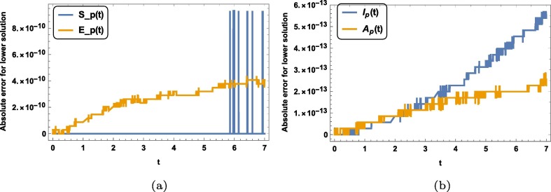
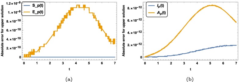
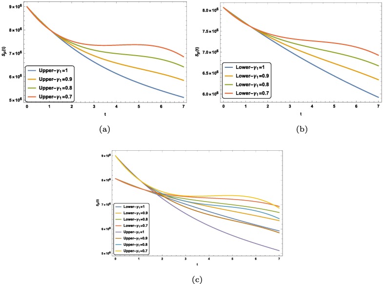
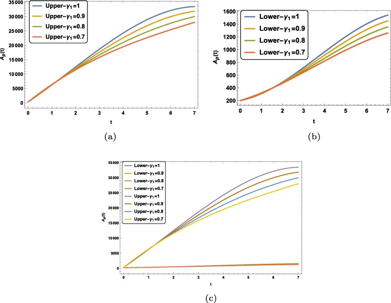
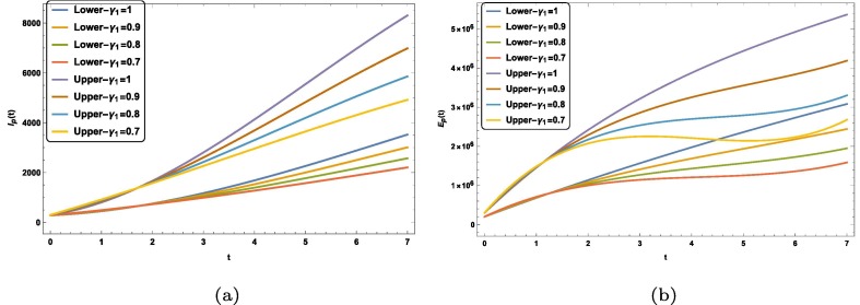
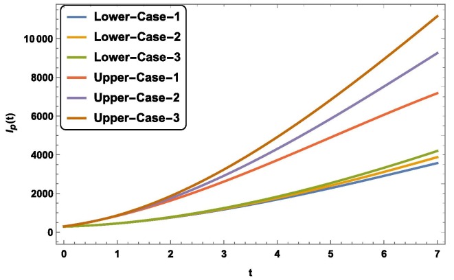
We see from the graphs of errors for different unknowns that our method is valid and feasible for a system of fuzzy fractional ordinary differential equations with Mittag–Leffler law. Now we study the dynamics of susceptible, exposed, infected and asymptotically infected people with different fractional order. Fig. 1 (a) is plotted between susceptible people versus time in case of upper solution and Fig. 1(b) is plotted between exposed people versus time in case of lower solution. We see in Fig. 1(a) and Fig. 1(b) both that number of exposed people increases with time. We observe that this growth increases as we increases the fractional order ${\gamma }_2$ from $0.7$ to 1. Fig. 2 (a) and Fig. 2(b) are plotted between asymptotically infected people $I_p\left(t\right)$ versus time in case of lower and upper solution. Fig. 2(a) and Fig. 2(b) predicts that number of asymptotically infected people will increase with time. Fig. 3 (a) and Fig. 3(b) represents the $S_p\left(t\right)$ for lower, upper and both solution for different fractional order for $N=4$. Fig. 4 (a) and Fig. 4(b) represents the $A_p\left(t\right)$ for lower, upper and both solution for different fractional order for $N=4$. Fig. 5 (a) and Fig. 5(b) represents the growth of infected people $I_p\left(t\right)$ and $E_p\left(t\right)$ with time, respectively. In both case lower and upper solution case this growth increases. And as fractional order increases from $0.7$ to integer order 1 this growth increases with order in both upper and lower case. Fig. 5(b) is plotted between fuzzy unknown function named as number of exposed people versus time. The number of exposed people increases like exponentially behavior with time and with increment in fractional order in both upper and lower case solution. To study the behavior of this virus with contacting to infected people, we plotted the graph between the infected people $I_p\left(t\right)$ versus time. We see in Fig. 6 that number of infected people increases with time. And an important fact can be seen that it increases as contact rate ${\eta }_p$ increases.

Fig. 1.

Variation of absolute error for susceptible, exposed, infected and asymptotically infected people in case of lower solution for N = 6.

Fig. 2.

Variation of absolute error for susceptible, exposed, infected and asymptotically infected people in case of upper solution for N = 6.

Fig. 3.

Graphical representation of $S_p\left(t\right)$ for lower, upper and both solution for different fractional order for $N=4$.

Fig. 4.

Graphical representation of $A_p\left(t\right)$ for lower, upper and both solution for different fractional order for $N=4$.

Fig. 5.

Graphical representation of $I_p\left(t\right)$ and $E_p\left(t\right)$ for different fractional order for $N=4$.

Fig. 6.

Graphical representation of $I_p\left(t\right)$ with different contact rate case1-$[0.05,0.1]$, case 2-$[50,100]$ and case 3-$[100,200]$ for $N=4$.

Conclusion

The present paper is devoted to numerical study of fractional mathematical model of COVID-19 in fuzzy environment. We have used the non-singular fractional derivative with Mittag–Leffler law. First of all, we derived the numerical approximation of fractional derivative of polynomial function ${(t-a)}^n$. By using this approximation we developed the operational matrix of fractional differentiation on domain $[0,a],a⩾1$. We solved COVID-19 model by using Legendre operational matrix. From the error graphs, we can conclude that our method is valid for a system of fuzzy fractional ordinary differential equation with Mittag–Leffler law and has a good accuracy. The dynamics of model with different fractional exponent is depicted by figures with showing the effect of fuzzy environment. The effect of contact rate on infected persons is also shown graphically. Our study is consistent with practical results which say this virus spread and no of infected people increases with increase in contact rate.

CRediT authorship contribution statement

A.A. Alderremy: Conceptualization, Methodology. J.F. Gómez-Aguilar: Conceptualization, Methodology, Writing - original draft, Software, Supervision. Shaban Aly: Data curation, Writing - original draft. Khaled M. Saad: Conceptualization, Methodology, Writing - original draft.

Declaration of Competing Interest

The authors declare that they have no known competing financial interests or personal relationships that could have appeared to influence the work reported in this paper.

References

- 1.Kilbas A., Srivastava H., Trujillo J.J. vol. 204. Amsterdam Amsterdam; Elsevier (North-Holland): 2006. (Theory and Applications of the Fractional Differential Equations). [Google Scholar]
- 2.Podlubny I. Academic Press; San Diego, CA: 1998. Fractional differential equations, to methods of their solution and some of their applications, Fractional Differential Equations: An Introduction to Fractional Derivatives. [Google Scholar]
- 3.Machado J.T., Kiryakova V., Mainardi F. Recent history of fractional calculus. Commun Nonlinear Sci Numer Simul. 2011;16(3):1140–1153. [Google Scholar]
- 4.Qureshi S., Yusuf A. Fractional derivatives applied to mseir problems: comparative study with real world data. Eur Phys J Plus. 2019;134:1–13. [Google Scholar]
- 5.Qureshi S., Yusuf A. Mathematical modeling for the impacts of deforestation on wildlife species using caputo differential operator. Chaos Solitons Fractals. 2019;126:32–40. [Google Scholar]
- 6.Qureshi S., Yusuf A. Modeling chickenpox disease with fractional derivatives: from caputo to atangana-baleanu. Chaos Solitons Fractals. 2019;122:111–118. [Google Scholar]
- 7.Darania P., Ebadian A. A method for the numerical solution of the integro-differential Eqs. 2007;188:657–668. [Google Scholar]
- 8.Suarez L, Shokooh A. An eigenvector expansion method for the solution of motion containing fractional derivatives 64 (1997).
- 9.Hashim I., Abdulaziz O., Momani S. Homotopy analysis method for fractional ivps. Commun Nonlinear Sci Numer Simul. 2009;14(3):674–684. [Google Scholar]
- 10.Li Y., Sun N. Numerical solution of fractional differential equations using the generalized block pulse operational matrix. Comput Math Appl. 2011;62(3):1046–1054. [Google Scholar]
- 11.Diethelm K., Ford N.J., Freed A.D. A predictor-corrector approach for the numerical solution of fractional differential equations. Nonlinear Dyn. 2002;29(1–4):3–22. [Google Scholar]
- 12.Li Y., Zhao W. Haar wavelet operational matrix of fractional order integration and its applications in solving the fractional order differential equations. Appl Math Comput. 2010;216(8):2276–2285. [Google Scholar]
- 13.Odibat Z. On legendre polynomial approximation with the vim or ham for numerical treatment of nonlinear fractional differential equations. J Comput Appl Math. 2011;235(9):2956–2968. [Google Scholar]
- 14.Jafari H., Yousefi S., Firoozjaee M., Momani S., Khalique C.M. Application of legendre wavelets for solving fractional differential equations. Comput Math Appl. 2011;62(3):1038–1045. [Google Scholar]
- 15.Yuanlu L. Solving a nonlinear fractional differential equation using chebyshev wavelets. Commun Nonlinear Sci Numer Simul. 2010;15(9):2284–2292. [Google Scholar]
- 16.Araci S. Novel identities for q-genocchi numbers and polynomials. J Function Spaces Appl. 2012;2012 [Google Scholar]
- 17.Gürbüz B., Sezer M. Laguerre polynomial solutions of a class of initial and boundary value problems arising in science and engineering fields. Acta Phys Pol, A. 2016;130(1):194–197. [Google Scholar]
- 18.Kaleva O. The calculus of fuzzy valued functions. Appl Math Lett. 1990;3(2):55–59. [Google Scholar]
- 19.Ahmadian A, Suleiman M, Salahshour S. An operational matrix based on legendre polynomials for solving fuzzy fractional-order differential equations. In: Abstract and Applied Analysis, vol. 2013, Hindawi; 2013.
- 20.Krätschmer V. Some complete metrics on spaces of fuzzy subsets. Fuzzy Sets Syst. 2002;130(3):357–365. [Google Scholar]
- 21.Goetschel R., Jr, Voxman W. Topological properties of fuzzy numbers. Fuzzy Sets Syst. 1983;10(1–3):87–99. [Google Scholar]
- 22.Long H.V., Son N.T.K., Tam H.T.T. The solvability of fuzzy fractional partial differential equations under caputo gh-differentiability. Fuzzy Sets Syst. 2017;309:35–63. [Google Scholar]
- 23.Atangana A., Koca I. Chaos in a simple nonlinear system with atangana–baleanu derivatives with fractional order. Chaos Solitons Fractals. 2016;89:447–454. [Google Scholar]
- 24.Atangana A., Gómez-Aguilar J. Numerical approximation of riemann-liouville definition of fractional derivative: From riemann-liouville to atangana-baleanu. Numer Methods Partial Differential Eqs. 2018;34(5):1502–1523. [Google Scholar]
- 25.Atangana A., Khan M.A. Validity of fractal derivative to capturing chaotic attractors. Chaos Solitons Fractals. 2019;126:50–59. [Google Scholar]
- 26.Khan M.A., Atangana A. Modeling the dynamics of novel coronavirus (2019-ncov) with fractional derivative. Alexand Eng J. 2020 [Google Scholar]