

Abstract
The widely spreading COVID-19 has caused thousands of hundreds of mortalities over the world in the past few months. Early diagnosis of the virus is of great significance for both of infected patients and doctors providing treatments. Chest Computerized tomography (CT) screening is one of the most straightforward techniques to detect pneumonia which was caused by the virus and thus to make the diagnosis. To facilitate the process of diagnosing COVID-19, we therefore developed a graph convolutional neural network ResGNet-C under ResGNet framework to automatically classify lung CT images into normal and confirmed pneumonia caused by COVID-19. In ResGNet-C, two by-products named NNet-C, ResNet101-C that showed high performance on detection of COVID-19 are simultaneously generated as well. Our best model ResGNet-C achieved an averaged accuracy at 0.9662 with an averaged sensitivity at 0.9733 and an averaged specificity at 0.9591 using five cross-validations on the dataset, which is comprised of 296 CT images. To our best knowledge, this is the first attempt at integrating graph knowledge into the COVID-19 classification task. Graphs are constructed according to the Euclidean distance between features extracted by our proposed ResNet101-C and then are encoded with the features to give the prediction results of CT images. Besides the high-performance system, which surpassed all state-of-the-art methods, our proposed graph construction method is simple, transferrable yet quite helpful for improving the performance of classifiers, as can be justified by the experimental results.
Keywords: COVID-19, Pneumonia, Graph neural network, ResGNet-C, Deep learning
1. Introduction
The outbreak of a new coronavirus, which was later named as COVID-19, has surprised the world with its high infectivity and fatality rate [1]. Currently, more than seven million people around the world have been diagnosed with the virus while more than 406 thousand of them have died because of the virus, until 9/June/2020. Due to the influence of the virus, millions of cities have locked down which severly caused the economy damage all over the world to slow the spreading of the virus as there is no vaccine available yet. Patients being infected may show symptoms like having fever, coughing in a few days and could develop into severe illness or even die quickly. An early diagnosis turns out to be the most effective way for the necessary treatment and stopping the spreading of the virus. Viral nucleic acid test and CT screening are the two most widely used techniques for clinical diagnosis. However, the viral nucleic acid test requires sophisticated devices and takes a long time to give the diagnostic result [2]. Additionally, the high false-negative rate indirectly facilitates the spread of the viral COVID-19. Compared to the viral nucleic acid test, chest CT images are reported of high sensitivity [3]. However, manual interpretation of CT scanned images is time-consuming and is unstable due to the personal experience of radiologists and artefacts such as fatigue. Therefore, developing an automated computer-aided diagnostic system with high accuracy is demanding.
Recent years, we have witnessed significant advancement of deep learning, which was highly featured by Convolutional neural network (CNN). In 2012, a new structured CNN named AlexNet showed incomparable superiority to other traditional methods on natural image classification task [4]. Later on, the performance of CNNs has been greatly improved thanks to the upgraded hardware and novel architectures. Compared to the Central Processing Unit (CPU), Graphics Processing Unit (GPU) shows more powerful parallel computing power in graphics processing. New generations of GPUs, which benefit from the advancement of Integrated Circuits (IC) and electron components, have been equipped with even stronger computation capability. Besides the improvement of hardware, structural innovations of CNNs considerably boosted the performance of the state-of-the-art networks. By increasing the depth and width of networks, GoogLeNet [5], a 22-layer network, more efficiently utilizes the computing resources in the network compared to the previously developed networks. However, one problem brought in by the increase of networks' depth and width is gradient vanishing in the training process. To mitigate the training difficulty, residual networks [6], which incorporated residual learning, achieved even better performance on ImageNet while the complexity remains lower than VGG [7]. Compared to traditional convolution, depthwise separable convolution produces fewer parameters when the same sizes of the generated output are given [8]. Novel convolution technique named dilated convolution was proposed to enable a larger receptive field of convolutional kernels without introducing extra parameters. Alongside the improved performance of CNNs, CNNs have also been widely used in engineering, business, medicine [9], [10], [11]. CNNs have demonstrated powerful capability on extracting and combining spatial features to form high-level features, which turn out to be more representative compared to manual-crafted features. Recently numerous reports also demonstrated the success of AI and machine learning [13], [14], [15], [16], [17], [18], [19], [20], [21], [22], and other applications on brain functional network [23], [24], [25], [26], [27], indoor detection [28], [29], fingerspelling [30], [31], [32], and image analysis [33]. However, the applications of CNNs are greatly hindered because the underlying relationships between each element are ignored. Graph convolutional neural network (GCN), which can better deal with graph-structured data, therefore, is receiving more attention from different areas. Each element in GCNs is taken as a node while the relationships between elements are denoted by edges. Aggregation of neighbourhood features is one of the keys that differentiates GCNs from CNNs. Given the advantages of GCNs, they have also been widely used in areas including image classification and semantic segmentation [12]. Considering the benefits of GCNs, we developed a high-performance system for the detection of COVID-19 based on GCNs. In this paper, we first proposed a novel ResGNet framework, and then we proposed three different models for the detection of COVID-19 when implemening models under the framework:
-
(i)
We first proposed ResNet101-C model, which takes ResNet101 as the backbone. The models ending with “-C” here and after stands for the classifiers that detect COVID-19. The purposes of the proposition of ResNet101-C are two folds. (a) ResNet101-C alone can be used to classify lung CT images into normal and pneumonia and therefore detect COVID-19. (b) More importantly, after training with the interested training set, ResNet101-C is enabled to extract more representative features for the rest two models NNet-C and ResGNet-C. We first add more layers to the top of ResNet101, which is close to the output, to obtain ResNet101-C and have it trained with the training set. High-level features of 128 dimensions are then extracted from the activation layer in the ResNet101-C for further classification though ResNet101-C alone can work as a classifier for the binary classification task here.
-
(ii)
NNet-C, a one-layer neural network, is a simple classifier that takes features extracted by ResNet101-C as input. Also, the proposition of NNet-C mainly comes from two parts. One is that NNet-C alone is a high-performance classifier on detection of pneumonia caused by COVID-19. Another main reason is that NNet-C, which shares the same architecture as the graph neural network (GNN) in ResGNet-C, can be used as the model for comparison with models built under ResGNet-C framework.
-
(iii)
ResGNet-C. In ResGNet-C, ResNet101-C is reutilized for feature extraction. Graphs of the extracted features are constructed accordingly and are then combined with the extracted features as the input to a 1-layer GNN in ResGNet-C for classification. To build graphs, images both in the train set and test set are divided into batches to obtain features in batches. In each batch of the train set, each feature is taken as one node of the graph while the edges between nodes are built according to the top k neighbours with the highest similarities. Inspired by [34], we hypothesis that there are edges between one node and other top k nearest nodes. The distance between nodes is measure by Euclidean distance while edges are quantified by the adjacency matrix. The 1-layer GNN, though shallow in terms of depth, however, showed powerful performance after trained with graph-combined features.
Experiments on our COVID-19 dataset demonstrated that our proposed ResGNet-C achieved the highest accuracy on the dataset by using the 5-cross-validations, which surpasses all of the state-of-the-art models. The contributions of this paper are mainly three-folds. One is that this is the first attempt to date to combine graph representation with CNN on COVID-19 detection. Another is that we proposed a ResGNet framework that easily integrates graph representation of features, which is also extendable to other diseases detection area. The last and most important one is that we developed three different models for the detection of COVID-19 while ResGNet-C performed best. This paper is organized as follows. In Section 2, we will briefly introduce the basic of GCN. Then we will move to implementations of ResGNet framework in Section 3. Experiment design and results will be presented in 4, 5, respectively, while we conclude this paper in Section 6.
2. Background
Our world has been flooded with countless data from areas of chemistry, biology and computer science. To represent the underlying relationships of data, graphs are widely used. GNNs are therefore developed to the process the graphs constructed based on the data. Given the graph G and one of its nodes n, GNNs can be represented as learnt functions that map G and n to vectors of reals:
| (1) |
where m is the dimension of Euclidean space [35].
GNNs can be extended to GCNs by introducing convolutions. There are considerable works that successfully built graphs for application of GCNs in various areas [12], [36]. A Text GCN was built in [37] that achieved better performance than the state-of-the-art techniques on text classification. The single text graph was created according to word-occurrence in the particular corpus. The recommendation system is another popular application scenario of GCN. In [38], authors encoded graph convolution with RNNs to mine possible pattern of users and items. There are also successful works of GCNs on medical image analysis. To overcome the shortcomings of patched-based in colorectal cancer grading, Yanning et el. proposed so-called CGC-Net that takes the nucleus in a histology image as nodes while cellular interactions are mapped as edges [39]. Another GCN for cervical cell classification was developed in [34]. k-means clustering is applied to features extracted by CNNs to acquire centroids, based on which each node is depicted by the nearest centroid. The element in the adjacency matrix is set to one when two nodes are found to be neighbours to each other according to the Euclidean distance.
As the global situation is worsening due to COVID-19, experts are devoted to solving the global issue collaboratively. To facilitate the detection of COVID-19, researchers from both clinical area [40], [41], [42] and computer science area [43], [44], [45] have contributed their valuable efforts. Bilateral pulmonary parenchyma ground-glass and consolidative pulmonary opacities are typical CT findings, which, therefore, could be determinants on making the diagnosis of COVID-19. It was found by Wang et al. [46] that multilobe lesions appeared in most patients while those lesions were usually shown in the peripheral zone and the central zone. Patchy shadows, ground-glass opacity and consolidation change are demonstrated among patients. Similar conclusions were found by Zhao et al. [47]. As pointed out by them, chest CT images of patients being infected by COVID-19 are highly featured by lungs that were in the presence of bilateral ground-glass lesions. The progressive lesions are, however, consolidations with no migratory lesions. In the computer science community, there are also considerable works that aim at giving reliable diagnostic results based on images. A deep learning model named (COVID-Net) feed with X-rays images was proposed to detect COVID-19 cases. The results on open source repositories showed promising results while the developed AI system is publically available. In [43], the authors developed a detection system by using inception blocks [5]. However, the accuracy, which was 0.7310, is still quite low compared to other existing models. In another work [44], the authors developed a 3D deep learning framework by deploying ResNet50 as the backbone. The sensitivity and specificity were also more than 0.90, which gave an overall accuracy of 0.96. Clinically, sensitivity is more important than specificity to some extent. In work [45], the author developed an automatic detection system that achieved 100% sensitivity.
Though experts are consolidated on providing diagnostic results in faster and more accurate ways. However, there are still many challenges ahead. For radiologists, artificial factors such as fatigue and personal experience would heavily harm the accuracy of the diagnostic results. Also, it is challenging for radiologists to provide accurate results in a limited time. For the automatic detection systems, high sensitivity for most of the systems is still one main obstacle that prevents them from gaining better accuracy given the complexity of images and other possible factors. Also, all of the methods mentioned above ignored to consider the underlying relation between each chest images. Considering this, we proposed our ResGNet framework to pave the way for future research on the application of GCN to the detection of COVID-19. Besides, two other models named ResNet101-C and NNet-C that showed certain capability on detection of COVID-19 are developed as well.
3. Methodology
3.1. Proposed framework: ResGNet
ResGNet frameworks, which is flexible for transplanting to different image classification tasks, consists of pre-trained CNNs for feature extraction and GNN for classification. The pre-trained CNNs could be trained on different image data sets and then be directly transferred to the classification task. However, many works showed that the performance of pre-trained CNNs would be significantly improved if they can be fine-tuned by datasets that are highly similar to the interested datasets [48], [49]. Considering this, the CNNs that are pre-trained on natural images are firstly trained on the concerned datasets. Therefore, the top layers, which are close to the output, of the pre-trained layers have to be modified. After training with the interested datasets, the pre-trained CNNs is then implemented in ResGNet framework. Though the pre-trained networks can be directly used for classification, the performance can be further improved by introducing GNN.
After feeding pre-trained networks with images, features can then be extracted from fully-connected layers in the network. We then take each feature as one node in graph G to build graph representation for GNN,. Graph G is paired with (V, E), where V denotes nodes in the graph while E is the set of edges [35]. For a node classification task, for each node in the graph while N is the number of nodes in the graph G. Therefore, stands for the edge between node and . As E is abstract, the adjacency matrix is used to depict the edges betweeen nodes. When there is an edge between nodes i and j, the corresponding location in the adjacency matrix is set to be one. We assume that there is an edge when the node falls into the top k nearest neighbours of another node according to Euclidean distance as shown in Fig. 1 . Compared to other graph generation model [50], our method of constructing structured graphs is simple and straightforward. Instead of iteratively updating nodes in the graph, we predefined the number of nodes according to batch size N while edges are updated concerning the adjacency matrix.
Fig. 1.

Graph construction.
Let the extracted features of our chest CT images be N×M, Xi and Xj 1 ×M corresponds to node i and node j in X, then distance Disij between node i and node j is calculated according to:
| (2) |
By introducing a knn search method, which looks for top k nearest neighbours with minimum Euclidean distance, we can find the closest top k nearest neighbours. Given node i and a vector of reals
| (3) |
we can find and record k neighbours by simply sorting . We used knn(Xi) to refer to the k nearest neighbours of node Xi. Therefore, the adjacency matrix is built as follows:
| (4) |
Correspondingly, a degree matrix D that has the same dimensions as A can be calculated according to the following equation:
| (5) |
where is the trace of degree matrix D. Given the features N×M in a GCN with multi-layers, node features are updated according to the following rule:
| (6) |
| (7) |
and stands for the nodes’ feature representation in (h + 1)th layer and hth layer, respectively. . Mh +1 is the dimension of feature representation in (h + 1)th layer. is the weights between hth layer and (h + 1) layer. (·) is the softmax activation function, which can be defined as:
| (8) |
N×N indicates the normalized adjacent matrix A. The process of normalizing A can be demonstrated as [51]:
| (9) |
As GNNs are usually no more than two layers [34], [51], we build a one layer GNN in this work. Bias term b is introduced to improve the performance of fitting. Therefore, we have:
| (10) |
Specifically,
| (11) |
which is the features extracted by pre-trained CNNs. The combination of features extracted by pre-trained networks and graph is the key of GNN in the proposed framework. However, we found it effective by simply multiplying with the extracted features, which means:
| (12) |
is then used as the input of GNN to optimize and . The error between and the expected output Y can be written as:
| (13) |
where is the ture category of feature j and is the predicted category of feature j. is then updated according to:
| (14) |
| (15) |
where is the momentum rate.
By training GNN with the combined input , we finally have a model under ResGNet framework. The pseudocode code of ResGNet model is given in Algorithm 1.
| Algorithm 1. Proposed ResGNet Framework |
|---|
| Step 1: Load pre-trained networks trained on ImageNet; |
| Step 2: Replace top layers with new top layers for the classification task; |
| Step 3: Train modified pre-trained network on the target dataset with predefined hyperparameters; |
| Step 4: Generate features through activation layers in the fine-tuned network; |
| Step 5: Divide the features into batches; |
| Step 6: Find top k nearest neighbours for each feature in the batches and build graphs; |
| Step 7: Combine features with graph representation by multiplying features with the normalized adjacency matrix ; |
| Step 8: Train GNN in ResGNet with the combined features and update parameters. |
We, therefore, implemented ResGNet-C under our proposed ResGNet framework. Simultaneously, we then have ResNet101-C for preliminary classification and feature extraction and NNet-C for further classification and comparison. Flow chart of constructing three models is shown in Fig. 2.
Fig. 2.

Acquisition of three models.
3.2. Proposed model 1: ResNet101-C
To obtain the pre-trained network under ResGNet framework, we choose to use ResNet101 to build ResNet101-C. The reason why we use ResNet101 as the backbone here is that ResNet101 showed powerful performance on the image classification task [6]. Same as other networks, ResNet101 includes convolution, batch normalization and pooling units. Convolution is implemented by multiplying images with sliding windows, namely convolution kernels. Usually, the group of convolution kernels increases and the size of output features decreases while the network goes into deeper. Convolutions are usually stacked to form convolution blocks where features within the block remain the same size as the input while the size shrinks due to a larger stride of convolution and pooling. Given the size of the input to convolution is
| (16) |
where CGI is the number of channels of the input, the size of convolutional kernels is defined as
| (17) |
where CGO is the number of channels of the output. If we have the stride of convolution CS and assume the size output is
| (18) |
then the numerical relationship between the size of output and input and kernels are:
| (19) |
Similarly, the size of features shrinks as well after max-pooling when the stride is greater than 1. By doing so, the more abstract features with much fewer dimensions can be extracted. However, what makes ResNet different from other networks was the proposed residual learning. Given identity Z and its mapping F(Z), it was assumed that the underlying mapping of features H(Z) after a series of stacked layers was related to F(Z) and Z by:
| (20) |
H(Z), therefore, can be represented by:
| (21) |
It was believed that H(Z) can then be optimized by optimizing mapping F(Z). Adding of F(Z) and Z is implemented by shortcut connections that skip several convolutional layers and have identity Z added to F(Z) directly.
To obtain ResNet101-C for the classification task, we inserted a dropout layer and two fully connected layers with 128-neurons and 2-neurons as output size between FC1000 layer and the Softmax layer in original ResNet101. Given that the original connections in ResNet101 are FC1000-softmax-classification, then the adapted connections are FC1000-Dropout-FC128-FC2-softmax-classification. Dropout layer is introduced to prevent the overfitting [52]. Also, FC128 is a transitional layer that prevents significant information loss, which could otherwise happen when inputting the features directly into the final FC2 layer. The pseudocode code of implementing ResNet101-C is given in Algorithm 2. By doing so, we can have the architecture of ResNet101-C in following Fig. 3 .
Fig. 3.
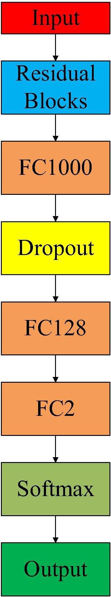
Architecture of ResNet101-C (Residual block denotes previous layers before FC1000 in the original ResNet101. FC1000, FC128 and FC2 are fully connected layers with output sizes of 1000, 128 and 2 respectively. Dropout layer drops part of connections between FC1000 and FC128 during the training session to prevent overfitting.).
| Algorithm 2. Implementation of ResNet101-C |
|---|
| Step 1: Load ResNet101 trained on ImageNet; |
| Step 2: Remove the top layers above FC1000 layer; |
| Step 3: Add a dropout layer as new top layers; |
| Step 4: Add FC128 and FC2 as new top layers; |
| Step 5: Add the softmax layer and classification layer for output, which gives ResNet101-C; |
| Step 6: Training ResNet101-C with the training set of COVID-19. |
| for i = 1: number_of_epochs |
| Step A: shuffle images in the train set |
| Step B: divide train set into batches |
| Step C: train ResNet101-C with each batch |
| end |
3.3. Proposed model 2: NNet-C
To provide a fair comparison with our GNN in ResGNet, we proposed a simple neural network NNet-C that has the same structure as our GNN while the main difference is the input. Given a batch of images , H, W, N stands for height, width, batch size, respectively. Then the output features of ResNet101-C can be obtained by:
| (22) |
where the features . is the operation of feature extraction by applying ResNet101-C. For NNet-C, the input is the features extracted by ResNet101-C in the layer FC128. Our GNN in ResGNet shares the same architecture of NNet-C while NNet-C is also an independent classifier. The architecture of NNet-C is shown in Fig. 4 .
Fig. 4.
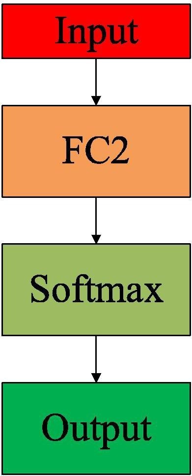
Architecture of NNet-C.
3.4. Proposed model 3: ResGNet-C
For COVID-19 detection, we term our model as ResGNet-C that was implemented under the proposed framework ResGNet. ResNet101-C is used to provide GNN in the proposed ResGNet-C with high-level features. “ResGNet101-C-FC128” means only layers including layer FC128 and before in ResGNet101-C in Fig. 5 are reutilized in ResGNet-C. In Fig. 5, the asterisk in the circle means the production of the adjacency matrix of graphs and features. The proposed GNN in ResGNet has the same structure as NNet-C while the main difference is GNN takes the combined features as input while the input of NNet-C is only the high-level features.
Fig. 5.

ResGNet-C.
3.5. Training
When training our proposed ResGNet-C, images have to be divided into batches while the size of batches N can be customized. Empirically, we set the batch size to be 2P, N = 2P. The details about choosing P will be presented in the experimental section. However, the number of images in the data set doesn’t necessarily to be divisible by the batch size N. Images in the second last batch will be reused in the last batch to make the size of the last batch to be N. The detailed process of acquiring each batch in the data set is shown in Fig. 6 . The top red bar denotes the sequence of images in the data set, which could either be the training set or test set. Given the number of images in the data set is O, the batch size is N, the number of batches
| (23) |
where is the ceiling operation.
Fig. 6.

Batch acquisition.
Each batch of images is first forwarded to ResNet101-C for feature acquisition. Then the graph within features is built by the aforementioned knn algorithm. By multiplying the normalized adjacency matrix with the features, the graph-combined features can then be forward to the classification layer to calculate the errors. The errors are then back-propagated to update the weights in GNN. The data flow of training data in the training period of three proposed models is shown in Fig. 7 . The pseudocode of training ResGNet-C is given in Algorithm 3.
| Algorithm 3. Training process of ResGNet-C |
|---|
| Step 1: Generate training features through ResNet101-C; |
| Step 2: for k = 1: number_of_epochs |
| for n = 1: STr (STr is the number of batches in the training set, which is calculated through equation (23) |
| Step A: Construct relation graph in each batch of features; |
| Step B: Combine features with graph; |
| Step C: forward combined features to GNN; |
| Step D: backwards the errors to update weights in GNN; |
| end |
| end |
| Step 3: Save and store the weights of ResGNet-C. |
Fig. 7.

Data flow of train set in three models.
3.6. Inference
In the inference phase, we followed a similar pattern to build and embed graphs. When inferring new images with the trained ResGNet-C, however, the size of batches is suggested to remain the same as the setting for the training set to maintain the best performance of the trained model. If there are no sufficient images for testing, samples from the training set can be utilized to form at least one batch of images. Details of inference are given in Algorithm 4.
| Algorithm 4. Testing process of ResGNet-C |
|---|
| Step 1: Load trained ResGNet-C; |
| Step 2: Generate testing features through ResNet101-C; |
| Step 3: Divide images in the test set into STe batches according to equation (23). |
| Step 4: Get the predicted categories for images in the test set. |
| for n = 1: STe |
| Step A: Construct graph for each batch of features; |
| Step B: Combine features with the graph; |
| Step C: forward combined features to GNN; |
| Step D: Get the predicted categories of each batch; |
| end |
| Step 5: Calculate the accuracy by comparing the predicted categories to real categories. |
4. Experiment design
4.1. Metrics of validation
When measuring the performance of our proposed models, five indicators including specificity, sensitivity, accuracy, precision, and F1 score, are used in our experiment. True Positive (TP), False Positive (FP), True Negative (TN) and False Negative (FN) are four main components involved in the calculation of the above indicators. TP indicates the number of correctly classified pneumonia caused by COVID-19; TN indicates the number of correctly classified normal images; FP indicates the number of images that are misclassified as pneumonia caused by COVID-19; FN indicates the number of images that are misclassified as normal.
Specificity reflects how our models perform on recognizing normal images from the test set and can be calculated through:
| (24) |
Sensitivity is the percentage of true positive (COVID-19 confirmed pneumonia) images that are correctly recognized and can be defined as:
| (25) |
Accuracy demonstrates the capability of our model on correct classification and can be written as:
| (26) |
Precision describes the percentage of predicted patients are true patients by
| (27) |
F1 score measures the classification ability:
| (28) |
4.2. Choice of best k and N
In ResGNet framework, N determines the sizes of graphs to be built while k determines the number of neighbours that should be consdered when calculating the adjacency matrix A in the graph. Therefore, the choice of k and N should be carefully chosen while training ResGNet-C. To choose the best k and N for our ResGNet-C, we vary both k and N until best k and N found. We use overall accuracy to measure the performance of GNN when different k and N are introduced.
| (29) |
where C(k, N) means the overall accuracy of GNN on test set when k and N are used as the number of neighbours and batch size respectively. k* and N* are the ideal values of k and N. The reason why we use the accuracy on test set is that we aimed at designing models that performed best on unseen data. The search domain of two variables are set as
| (30) |
| (31) |
where stands for the lower bound and upper bound of k. and stands for the lower bound and upper bound of N. The relationship between k and N is that k < N. In total, seven variables, shown in Table 1 , are defined in our algorithm. Details of searching for k* and N* can be seen in Algorithm 5.
| Algorithm 5. Choice of optimal k and N for knn |
|---|
| Criterion: C = Overall Accuracy on the test set |
| Objective Function: See equation (29). |
| Search domain: See equations (30) and (31). |
| Procedures: |
| Step 0: Variable Allocation |
| See Table 1. |
| Step 1: Initialization |
| Initialize k*, k with kLB, |
| k* = k = kLB |
| Initialize N*, N with NLB. |
| N* = N = NLB |
| Initialize variable Current_Accuracy = 0 |
| Set the increment stride of k to be and the stride of N to be . |
| Step 2: Retrain |
| Train GNN with k, N and obtain C(k, N) on test set; |
| Step 3: Update Current_Accuracy & k* & N* |
| if C(k, N) > % find a better solution |
| ; |
| k* = k; |
| N* = N; |
| end |
| Step 4: Update k |
| if (k + < kUB) && (k + < N) |
| k = k + ; |
| Then go back to Step 2; |
| else |
| Go to Step 5; |
| end |
| Step 5: Update N |
| if N + < |
| N = N + ; |
| Then go back to Step 2; |
| else |
| Go to Step 6; |
| end |
| Step 6: Output k* and N*. |
When inference the test images, all of the test images are fed to trained ResNet101-C to get the features. These features can be directly forwarded to NNet-C for classification without partitioning into batches. However, they have to be divided into batches for GNN in ResGNet-C because graphs between features nodes have to be built in a batch-wise form. But the order of images in the test set doesn’t necessarily to be the same when repeatedly redoing test on same test images. The graph representations are robust and are intrinsic with the features of images. Therefore, images in the train set can be sampled to form a batch of the testing images when there are not enough images to be classified.
Table 1.
Variable allocation in optimal k and N for knn algorithm.
| Variable name | Meaning |
|---|---|
| k | Number of neighbours considered |
| A constant denotes the increment stride of k | |
| k* | The variable that stores the best k so far |
| N | Batch size |
| A constant value denotes the increment stride of N | |
| N* | The variable that stores the best N so far |
| Current_Accuracy | A variable that stores the highest accuracy on the test set so far. |
4.3. Experiment setting
In this paper, all of the experiments are carried out on a personal laptop with 16G RAM and GPU GTX1050. There are two sets of parameters for training ResNet101-C, NNet-C and GNN in ResGNet-C. When training ResNet101-C, we have 40 as maximum training epochs, initial learning rate 10−4, batch size 8. The initial learning rate is 10−4 while it halves every five epochs. The stochastic gradient descent with momentum (SGDM) is used as an optimization algorithm. During the training session, the train set shuffles at every epoch. NNet-C is trained with the same hyperparameters. Details are shown in Table 2 .
Table 2.
Hyperparameters of ResNet101-C and NNet-C.
| Parameter | Value |
|---|---|
| Maximum training epoch | 40 |
| Initial learning rate | 10-4 |
| Batch size | 8 |
| Learning rate drop period | 5 |
| Learning rate drop rate | 0.5 |
| Optimization method | SGDM |
| Shuffle of the train set | Each epoch |
The training parameters for GNN are set throughout all of the experiments if no other specifications are given. Batch size and number of neighbours in knn algorithm are two parameters that could significantly affect the performance of ResGNet. The maximum training epoch is 40. When training our GNN with extracted features, the training set shuffles each epoch. Considering that the size of the testing is small, we set the following parameters when searching for best k and N, as can be seen in Table 3 . It would be meaningless when k UB is too close to N, we, therefore, defined the upper bound according to N by:
| (32) |
Table 3.
Hyperparameters of GNN.
| Parameter | Value |
|---|---|
| Lower bound NLB | 16 |
| Upper bound NUB | 32 |
| Stride | 16 |
| Lower bound kLB | 3 |
| Upper bound kUB | |
| Stride ks | 4 |
| Maximum training epoch | 40 |
| Initial learning rate | 10-4 |
| Learning rate drop period | 5 |
| Learning rate drop rate | 0.5 |
| Optimization method | SGDM |
| Shuffle of the train set | Each epoch |
5. Results and discussions
In this section, we will have a detailed introduction to the dataset used in this research, followed by metrics of validation used in the research. To design the best ResGNet model, we tried different batch size N and the number of neighbours k to determine the best parameters for the COVID-19 detection task. By having an internal comparison within three proposed models, it was justified that ResGNet-C performed best though it has great similarity to ResNet101-C and NNet-C on certain aspects. We end up this section by comparing our ResGNet-C with the state-of-the-art methods and found that our ResGNet-C still performs best among all of the methods compared.
5.1. Dataset acquisition
There are in total of 132 cases utilized for analysis in this research. 66 of them, who have confirmed pneumonia caused COVID-19 by the Fourth People’s Hospital of Huai’an City, contributed 148 CT scans that are scanned between January 2020 and March 2020. To balance the data set, we used another 148 CT scans from 66 cases that are randomly selected from 159 healthy examiners. The instrument and settings for CT acquisition are Philips Ingenity 64 row spiral CT machine, Mas:240, KV:120, layer spacing 3 mm, layer thickness 3 mm, Mediastinum window (W: 350, L: 60), thin layer reconstruction according to the lesion display. Two experienced radiologists collaboratively read the radiographs to provide the diagnostic results. When there are disagreements on the diagnostic results, a third radiologist is involved in reaching consensus. Each slice of CT scans is selected based on the following rules: The largest level of the lesions caused by COVID-19 are ensured to be presented in the COVID-19 confirmed images while a random level of the image is selected for normal examiners. Two examples of the images in the data set are given in Fig. 8 below.
Fig. 8.

Sample of images.
Five cross-validation method was deployed to validate the effectiveness of our proposed models. Therefore, 80% of images were portioned into the train set, while 20% left for testing. Details about the train set and test set are given in Table 4 . In each trial of cross-validation, the number of images in the test set is either 58 or 60. The reason why the number varies is that the total number of images in the dataset, which is 296, can not be perfectly divided into 5 batches that of the same size, which results in some batches have 1 or 2 fewer images than the rest of the batches. Therefore, numbers of images in the train set and the test set vary slightly.
Table 4.
Composition of training and test set of each trial.
| Set | COVID-19 | Healthy | Total |
|---|---|---|---|
| Training | 118(119) | 118(119) | 236(238) |
| Test | 30(29) | 30(29) | 60(58) |
| Total | 148 | 148 | 296 |
a(b) represents the number of images may vary from a to b.
5.2. Exploration of the best k and N
When N = 16, the results are given shown in Table 5 . In Table 5 and onwards, bold font indicates the most desirable results. Interestingly, the best performance achieved when batch size N is 16 while k = 3. However, the accuracy of ResGet-C seems to fluctuate when k increases though the Sensitivity increases when k becomes larger. To search for the best k and N in the search domain, we presented the results of classification when N = 32 in Table 6 .
Table 5.
Performance of ResGNet-C when batch size N = 16, k = 3, 7, 11.
| k | Specificity | Sensitivity | F1 | Precision | Accuracy |
|---|---|---|---|---|---|
| 3 | 0.9933 ± 0.0149 | 0.9248 ± 0.0959 | 0.9555 ± 0.0524 | 0.9935 ± 0.0144 | 0.9591 ± 0.0452 |
| 7 | 0.8864 ± 0.1625 | 0.9655 ± 0.0771 | 0.9315 ± 0.0624 | 0.9112 ± 0.1130 | 0.9260 ± 0.0751 |
| 11 | 0.9393 ± 0.0375 | 0.9724 ± 0.0617 | 0.9560 ± 0.0183 | 0.9437 ± 0.0342 | 0.9559 ± 0.0160 |
Table 6.
Performance of ResGNet-C when batch size N = 32 and k = 3, 7, 11, 15, 19, 23, 27.
| k | Specificity | Sensitivity | F1 | Precision | Accuracy |
|---|---|---|---|---|---|
| 3 | 0.9467 ± 0.0691 | 0.9115 ± 0.1133 | 0.9255 ± 0.0633 | 0.9501 ± 0.0626 | 0.9291 ± 0.0571 |
| 7 | 0.9591 ± 0.0446 | 0.9733 ± 0.0365 | 0.9665 ± 0.0114 | 0.9621 ± 0.0407 | 0.9662 ± 0.0122 |
| 11 | 0.9462 ± 0.0301 | 0.9448 ± 0.1234 | 0.9420 ± 0.0570 | 0.9496 ± 0.0282 | 0.9455 ± 0.0467 |
| 15 | 0.9126 ± 0.0732 | 0.9586 ± 0.0925 | 0.9360 ± 0.0374 | 0.9229 ± 0.0606 | 0.9356 ± 0.0349 |
| 19 | 0.9260 ± 0.0499 | 0.9241 ± 0.1696 | 0.9180 ± 0.0859 | 0.9327 ± 0.0442 | 0.9251 ± 0.0656 |
| 23 | 0.9120 ± 0.0196 | 0.9517 ± 0.1079 | 0.9307 ± 0.0653 | 0.9141 ± 0.0242 | 0.9318 ± 0.0589 |
| 27 | 0.9186 ± 0.0201 | 1.0000 ± 0.0000 | 0.9610 ± 0.0093 | 0.9250 ± 0.0171 | 0.9593 ± 0.0101 |
As can be seen, all models with different nearest k neighbours showed over 0.92 accuracies on the classification task here while the model with k = 7 performed best. Also, the accuracy indicates that the performance of the ResGNet-C is not proportional to k but turns out to be best when a proper number of k is chosen.
Also, we noticed that ResGNet-C performed best when k is 0.25*k − 1 of batch size as it was coherent in Fig. 9 . Surprisingly, the sensitivity increases with k while the batch size is fixed. However, the specificity decreases when k increases. Therefore, we may roughly conclude that models trained with different parameters sacrifice specificity for sensitivity when k increases. Therefore, a pair of best k and N that gives the best model can be found. And from the above experiment, we found that the proposed ResGNet-C model performed best when k is 7 while N is fixed to be 32. For the experiment afterwards, we fixed batch size to be 32 while the k is fixed at 7 if there is no other specification.
Fig. 9.

Error bar of choices of best k and N.
5.3. Method comparison
We also internally compared three proposed models. As mentioned before, both of GNN in ResGNet and NNet-C are trained with the same parameters and feed with same features extracted by ResNet101-C. Also, we compared our ResGNet-C with the ResNet101-C to prove the improvement of performance. The simplified receiver operating characteristic curves (ROC) of three models are given in Fig. 10 . The performance of the three models is given in Table 7 and Fig. 11 .
Fig. 10.

The simplified Receiver Operating Characteristic curves of models.
Table 7.
Performance of three proposed models.
| Model | Specificity | Sensitivity | F1 | Precision | Accuracy |
|---|---|---|---|---|---|
| NNet-C (Ours) | 0.8575 ± 0.1186 | 0.8044 ± 0.0949 | 0.8262 ± 0.0648 | 0.8592 ± 0.0916 | 0.8309 ± 0.0659 |
| ResNet101-C (Ours) | 0.9733 ± 0.0365 | 0.8584 ± 0.0354 | 0.9107 ± 0.0347 | 0.9703 ± 0.0407 | 0.9159 ± 0.0326 |
| ResGNet-C (Ours) | 0.9591 ± 0.0446 | 0.9733 ± 0.0365 | 0.9665 ± 0.0114 | 0.9621 ± 0.0407 | 0.9662 ± 0.0122 |
Fig. 11.

Comparison of three proposed models.
As can be seen from the Fig. 10, the ResNet101-C has already achieved high sensitivity, which contributed to the overall good performance on classification. However, the performance of NNet-C becomes even worse.
The reason could be the training parameters are not optimal in terms of feature classification. The other possible reason is the simplicity of NNet-C, which only has no hidden layer but 2 neurons in the last layer. Nevertheless, our proposed ResGNet-C performed best amongst all three models though GNN has the same structure as NNet-C.
It is worth notifying that the accuracy of our model has been significantly increased compared to the accuracy of NNet-C, even surpassed the accuracy of ResNet101-C by a big margin. Therefore, integrating the graph into the classification turns out to be reasonable and helpful. The simplified ROC curves also implied that our proposed method of graph construction is plausible and simple to implement.
5.4. Comparison of our method and state-of-the-art methods
To further validate our proposed ResGNet-C, we compared our method with state-of-the-art methods. The results are given in Table 8 below. Our model performed best in terms of specificity, F1 score, precision, and overall accuracy. Though sensitivity is quite high while comparable to 100%, which is promising via a five cross-validation on the dataset.
Table 8.
Comparison with SOTA methods.
| Model | Specificity | Sensitivity | F1 | Precision | Accuracy |
|---|---|---|---|---|---|
| K-ELM [53] | 0.5682 | 0.6136 | 0.5952 | 0.5909 | 0.5814 |
| ELM-BA [54] | 0.5500 ± 0.0258 | 0.7636 ± 0.0244 | 0.6997 ± 0.0244 | 0.6568 ± 0.0192 | 0.6156 ± 0.0225 |
| Wang [43] | 0. 6700 | 0.7400 | – | – | 0.7310 |
| Li [44] | 0.9000 | 0.9600 | – | – | 0.9600 |
| Mangal [45] | – | 1.0000 | – | – | 0.9050 |
| ResGNet-C (Ours) | 0.9591 ± 0.0446 | 0.9733 ± 0.0365 | 0.9665 ± 0.0114 | 0.9621 ± 0.0407 | 0.9662 ± 0.0122 |
The reasons why ResGNet-C performed best amongst all of the methods are mainly two folds. One is the architectural superiority of ResNet101-C that extracted enough representative features. As can be seen from Table 7, ResNet101-C has achieved an average accuracy at 0.9159, which is already higher than most of the state-of-the-art methods. The other reason is the feature embedding of GNN. As there is no structural difference between NNet-C and GNN, graphs built serve to enhance the features by combining the underlying relationships between features.
In this paper, we proposed a new graph convolutional neural network framework named ResGNet for the detection of pneumonia caused by COVID-19. The key of building ResGNet-C under the framework was to choose the best number of neighbours k and batch size N. By training ResGNet-C for multiple times with different values of k and N, best k and N were chosen when trained ResGNet-C performed best on the test set. To ensure a best-performed model on the test set, transductive learning has been widely used [55], [56]. In transductive learning, samples in the train set and test set are not individually considered for labelling or for classification. Instead, information of neighbours, whether neighbours are in train set or in the test set, is introduced to guide the model to give more desirable results on the test set. Similarly, in our proposed framework, we borrowed the idea of using neighbour information to direct the proposed GNN towards better performance. However, the difference is that we used local neighbour information that is extracted from neighbours that belong to the same batch of the interested sample. Also, in our case here, samples in the test set are completely hidden during the training period, which differentiates our inductive model from the transductive model in the beginning.
6. Conclusion
In this paper, we developed an effective COVID-19 detection system with high sensitivity and specificity. ResGNet, which is a GCN with novel network architecture, is proposed to extract representative features and to classify features into being healthy and being infected. The residual network ResNet101 is used to create ResNet101-C for its high performance on features extracting. By reutilizing ResNet101-C, features are extracted for the graph construction, which contributes to improving the performance of the subsequent GNN in ResGNet-C. It is the first attempt at combining graph knowledge into the detection of COVID-19 and could be the cornerstone for future research. The method we proposed to build the graph is quite simple yet adaptive, which can be easily transplanted to other similar works. Experiments also supported our graph-construction method and the proposed models.
However, there are also some limitations to our work. One is the limited number of images in this research, which indirectly constrains the performance of our models. Also, the search domain of the size of batch N and the number of neighbours k needs further explorations and will be listed in our future works.
CRediT authorship contribution statement
Xiang Yu: Conceptualization, Methodology, Software, Writing - review & editing. Siyuan Lu: Writing - review & editing, Visualization. Lili Guo: Data curation. Shui-Hua Wang: Methodology, Writing - review & editing, Supervision, Validation. Yu-Dong Zhang: Conceptualization, Writing - review & editing, Investigation, Supervision, Validation, Writing - review & editing.
Declaration of Competing Interest
The authors declare that they have no known competing financial interests or personal relationships that could have appeared to influence the work reported in this paper.
Acknowledgement
This paper was supported by Royal Society International Exchanges Cost Share Award, UK (RP202G0230), Medical Research Council Confidence in Concept Award, UK (MC_PC_17171), Hope Foundation for Cancer Research, UK (RM60G0680), British Heart Foundation Accelerator Award, UK; Fundamental Research Funds for the Central Universities (CDLS-2020-03); Key Laboratory of Child Development and Learning Science (Southeast University), Ministry of Education; Guangxi Key Laboratory of Trusted Software (kx201901). Also, Xiang Yu and Siyuan Lu hold CSC scholarship with the University of Leicester.
Biographies
Xiang Yu received his bachelor degree and master degree from Huanggang Normal University and Xiamen University, P.R. China, in 2014 and 2018, respectively. Currently, he is a Ph.D. student in the Department of Informatics, University of Leicester, UK. Also, he was sponsored by CSC and by the University of Leicester as a graduate teaching assistant (GTA). His research interests include medical image segmentation, machine learning and deep learning.
Siyuan Lu received B.S. and M.S. in Nanjing Normal University of Computer Science & Technology 2014 and 2018 respectively. Now He is a PhD candidate in University of Leicester, department of informatics, majoring in image processing and machine learning.
Professor Lili Guo received a bachelor's degree in medical imaging in 2001 and a master's degree in medical imaging in 2007 from Xuzhou Medical College. She received M.D. in medical imaging from Nanjing Medical University in 2016. She worked as postdoc from 2019 in the department of medical imaging of Jinling Hospital. She is currently the director of the CT Department of the affiliated Huai'an No.1 People’s Hospital of Nanjing Medical University and as an Associate Professor and master tutor of Nanjing Medical University. She has conducted several provincial and municipal scientific research projects and published more than 20 papers. The main research interests include the application of radiomics and deep learning in imaging.
Dr. Shui-Hua Wang got her bachelor’s degree in Information Sciences from Southeast University, Nanjing, China in 2008, master’s degree in Electrical Engineering from City college of New York, New York, USA in 2012, and Ph.D. degree in Electrical Engineering from Nanjing University, Nanjing, China in 2017. She worked as an Assistant Professor in Nanjing Normal University from 2013-2018. She also served as Research Associate in Loughborough University from 2018-2019. Now, she is working as Research Associate in University of Leicester, UK. She is currently serving as Guest Editor-in-Chief of Multimedia Systems and Applications, Associate editor of Journal of Alzheimer’s Disease, IEEE Access, IEEE Transactions on Circuits and Systems for Video Technology (TCSVT). Dr. Shui-Hua Wang is a member of IEEE from 2011 and China Computer Federation from 2015. She was rewarded as the Highly cited researchers 2019. She published over 100 papers, including 10 “ESI Highly Cited Papers”. Her citation reached 8052 in Google Scholar, and 4628 in Web of Science. She has conducted many successful industrial projects and academic grants from British Heart Foundation, Nature Science Foundation of China, Royal Society.
Prof. Yu-Dong Zhang received his BE in Information Sciences in 2004, and MPhil in Communication and Information Engineering in 2007, from Nanjing University of Aeronautics and Astronautics. He received the PhD degree in Signal and Information Processing from Southeast University in 2010. He worked as a postdoc from 2010 to 2012 with Columbia University, USA; and as an assistant research scientist from 2012 to 2013 with Research Foundation of Mental Hygiene (RFMH), USA. He served as a full professor from 2013 to 2017 with Nanjing Normal University. Now he serves as Professor with Department of Informatics, University of Leicester, UK. He is the author of over 200 articles. His research interests include deep learning and medical image analysis. He is the editor of Neural Networks, Scientific Reports, IEEE Transactions on Circuits and Systems for Video Technology, etc. Prof. Zhang is the fellow of IET (FIET), and the senior members of IEEE and ACM. He was included in “Most Cited Chinese researchers (Computer Science)” by Elsevier from 2014 to 2018. He was the 2019 recipient of “Highly Cited Researcher” by Web of Science. His citation reached 10799 in Google Scholar, and 5787 in Web of Science. He has conducted many successful industrial projects and academic grants from NSFC, NIH, Royal Society, EPSRC, MRC, and British Council.
Communicated by D.-S. Huang
References
- 1.Baud D., Qi X., Nielsen-Saines K., Musso D., Pomar L., Favre G. Real estimates of mortality following COVID-19 infection. Lancet Infect. Diseases. 2020 doi: 10.1016/S1473-3099(20)30195-X. [DOI] [PMC free article] [PubMed] [Google Scholar]
- 2.Y. Li, L. Xia, Coronavirus Disease 2019 (COVID-19): Role of chest CT in diagnosis and management, Am. J. Roentgenol. (2020) 1–7. [DOI] [PubMed]
- 3.Y. Fang, et al., Sensitivity of chest CT for COVID-19: comparison to RT-PCR, Radiology (2020) 200432. [DOI] [PMC free article] [PubMed]
- 4.S.I. Krizhevsky Alex, H.G. E, Imagenet classification with deep convolutional neural networks, in: Advances in Neural Information Processing Systems, 2012, pp. 1097–1105.
- 5.L. W. Szegedy Christian, Yangqing Jia, Pierre Sermanet, Scott Reed, Dragomir Anguelov, Dumitru Erhan, Going deeper with convolutions, in: Proceedings of the IEEE Conference on Computer Vision and Pattern Recognition, 2015, pp. 1–9
- 6.K. He, X. Zhang, S. Ren, J. Sun, Deep residual learning for image recognition, in: Proceedings of the IEEE Conference on Computer Vision and Pattern Recognition, 2016, pp. 770–778
- 7.Z.A. Simonyan Karen, Very deep convolutional networks for large-scale image recognition, arXiv, 2014
- 8.A.G. Howard, et al., Mobilenets: efficient convolutional neural networks for mobile vision applications, arXiv preprint arXiv:1704.04861, 2017.
- 9.Young T., Hazarika D., Poria S., Cambria E. Recent trends in deep learning based natural language processing. IEEE Comput. Intell. Mag. 2018;13(3):55–75. [Google Scholar]
- 10.Badrinarayanan V., Kendall A., Cipolla R. Segnet: a deep convolutional encoder-decoder architecture for image segmentation. IEEE Trans. Pattern Anal. Mach. Intell. 2017;39(12):2481–2495. doi: 10.1109/TPAMI.2016.2644615. [DOI] [PubMed] [Google Scholar]
- 11.H. Jiang, E. Learned-Miller, Face detection with the faster R-CNN, in: 2017 12th IEEE International Conference on Automatic Face & Gesture Recognition (FG 2017), 2017, IEEE, pp. 650–657
- 12.J. Zhou, et al., Graph neural networks: a review of methods and applications, arXiv preprint arXiv:1812.08434, 2018.
- 13.D.-S. Huang, Systematic theory of neural networks for pattern recognition, Publishing House of Electronic Industry of China, Beijing, vol. 201, 1996.
- 14.Huang D.-S. Radial basis probabilistic neural networks: model and application. Int. J. Pattern Recognit. Artif. Intell. 1999;13(07):1083–1101. [Google Scholar]
- 15.Huang D.-S. A constructive approach for finding arbitrary roots of polynomials by neural networks. IEEE Trans. Neural Networks. 2004;15(2):477–491. doi: 10.1109/TNN.2004.824424. [DOI] [PubMed] [Google Scholar]
- 16.Huang D.-S., Du J.-X. A constructive hybrid structure optimization methodology for radial basis probabilistic neural networks. IEEE Trans. Neural Networks. 2008;19(12):2099–2115. doi: 10.1109/TNN.2008.2004370. [DOI] [PubMed] [Google Scholar]
- 17.Huang D.-S., Ip H.H., Chi Z. A neural root finder of polynomials based on root moments. Neural Comput. 2004;16(8):1721–1762. [Google Scholar]
- 18.Huang D.-S., Ip H.-H.-S., Law K.C.K., Chi Z. Zeroing polynomials using modified constrained neural network approach. IEEE Trans. Neural Networks. 2005;16(3):721–732. doi: 10.1109/TNN.2005.844912. [DOI] [PubMed] [Google Scholar]
- 19.Huang D.-S., Jiang W. A general CPL-AdS methodology for fixing dynamic parameters in dual environments. IEEE Trans. Syst. Man Cybern. B (Cybern.) 2012;42(5):1489–1500. doi: 10.1109/TSMCB.2012.2192475. [DOI] [PubMed] [Google Scholar]
- 20.Wang X.-F., Huang D.-S. A novel density-based clustering framework by using level set method. IEEE Trans. Knowl. Data Eng. 2009;21(11):1515–1531. [Google Scholar]
- 21.Wang X.-F., Huang D.-S., Xu H. An efficient local Chan-Vese model for image segmentation. Pattern Recogn. 2010;43(3):603–618. [Google Scholar]
- 22.Zhao Z.-Q., Glotin H., Xie Z., Gao J., Wu X. Cooperative sparse representation in two opposite directions for semi-supervised image annotation. IEEE Trans. Image Process. 2012;21(9):4218–4231. doi: 10.1109/TIP.2012.2197631. [DOI] [PubMed] [Google Scholar]
- 23.Jiao Z., Ji Y., Jiao T., Wang S.-H. Extracting sub-networks from brain functional network using graph regularized nonnegative matrix factorization. Comput. Model. Eng. Sci. 2020;123(2):845–871. [Google Scholar]
- 24.Jiao Z., Xia Z., Cai M., Zou L., Xiang J., Wang S. Hub recognition for brain functional networks by using multiple-feature combination. Comput. Electr. Eng. 2018;69:740–752. [Google Scholar]
- 25.Jiao Z., Xia Z., Ming X., Cheng C., Wang S.-H. Multi-scale feature combination of brain functional network for eMCI classification. IEEE Access. 2019;7:74263–74273. [Google Scholar]
- 26.Jiao Z.-Q., Zou L., Cao Y., Qian N., Ma Z.-H. Effective connectivity analysis of fMRI data based on network motifs. J. Supercomput. 2014;67(3):806–819. [Google Scholar]
- 27.Jiao Z., Ma K., Wang H., Zou L., Zhang Y. Research on node properties of resting-state brain functional networks by using node activity and ALFF. Multimedia Tools Appl. 2018;77(17):22689–22704. [Google Scholar]
- 28.Xu Y., Ahn C.K., Shmaliy Y.S., Chen X., Li Y. Adaptive robust INS/UWB-integrated human tracking using UFIR filter bank. Measurement. 2018;123:1–7. [Google Scholar]
- 29.Xu Y., Li Y., Ahn C.K., Chen X. Seamless indoor pedestrian tracking by fusing INS and UWB measurements via LS-SVM assisted UFIR filter. Neurocomputing. 2020 [Google Scholar]
- 30.X. Jiang, Fingerspelling identification for Chinese sign language via AlexNet-based transfer learning and Adam optimizer, Sci. Program. 2020 (2020) Art No. 3291426.
- 31.Jiang X., Chang L. Classification of Alzheimer’s disease via eight-layer convolutional neural network with batch normalization and dropout techniques. J. Med. Imag. Health Inf. 2020;10(5):1040–1048. [Google Scholar]
- 32.X. Jiang, Z. Zhu, M. Zhang, Recognition of Chinese finger sign language via gray-level co-occurrence matrix and K-nearest neighbor algorithm, in: 3rd International Conference on Electronic Information Technology and Computer Engineering (EITCE), Xiamen, China, 18–20 Oct. 2019, IEEE, pp. 152–156. doi: 10.1109/EITCE47263.2019.9094915.
- 33.C. Tang, E. Lee, Hearing loss identification via wavelet entropy and combination of Tabu search and particle swarm optimization, in: 23rd International Conference on Digital Signal Processing (DSP), Shanghai, China, 2018, IEEE, pp. 1–5.
- 34.J. Shi, R. Wang, Y. Zheng, Z. Jiang, L. Yu, Graph Convolutional Networks for Cervical Cell Classification, 2019 [DOI] [PubMed]
- 35.Scarselli F., Gori M., Tsoi A.C., Hagenbuchner M., Monfardini G. The graph neural network model. IEEE Trans. Neural Networks. 2008;20(1):61–80. doi: 10.1109/TNN.2008.2005605. [DOI] [PubMed] [Google Scholar]
- 36.Z. Wu, S. Pan, F. Chen, G. Long, C. Zhang, S.Y. Philip, A comprehensive survey on graph neural networks, IEEE Trans. Neural Networks Learn. Syst. (2020). [DOI] [PubMed]
- 37.L. Yao, C. Mao, Y. Luo, Graph convolutional networks for text classification, in: Proceedings of the AAAI Conference on Artificial Intelligence, 2019, vol. 33, pp. 7370–7377
- 38.Monti F., Bronstein M., Bresson X. Geometric matrix completion with recurrent multi-graph neural networks. Adv. Neural Inf. Process. Syst. 2017:3697–3707. [Google Scholar]
- 39.Y. Zhou, S. Graham, N. Alemi Koohbanani, M. Shaban, P.-A. Heng, N. Rajpoot, Cgc-net: cell graph convolutional network for grading of colorectal cancer histology images, in: Proceedings of the IEEE International Conference on Computer Vision Workshops, 2019, pp. 0–0
- 40.Chung M., et al. CT imaging features of 2019 novel coronavirus (2019-nCoV) Radiology. 2020;295(1):202–207. doi: 10.1148/radiol.2020200230. [DOI] [PMC free article] [PubMed] [Google Scholar]
- 41.S. Yang, et al., Clinical and CT features of early-stage patients with COVID-19: a retrospective analysis of imported cases in Shanghai, China, Eur. Respirat. J. (2020) 2000407. doi: 10.1183/13993003.00407-2020. [DOI] [PMC free article] [PubMed]
- 42.Huang G., et al. Timely diagnosis and treatment shortens the time to resolution of coronavirus disease (COVID-19) pneumonia and lowers the highest and last CT scores from sequential chest CT. Am. J. Roentgenol. 2020:1–7. doi: 10.2214/AJR.20.23078. [DOI] [PubMed] [Google Scholar]
- 43.S. Wang, et al., A deep learning algorithm using CT images to screen for Corona Virus Disease (COVID-19), medRxiv, 2020 [DOI] [PMC free article] [PubMed]
- 44.L. Li, et al., Artificial intelligence distinguishes covid-19 from community acquired pneumonia on chest ct, Radiology (2020) 200905.
- 45.A. Mangal, et al., CovidAID: COVID-19 Detection Using Chest X-Ray, arXiv preprint arXiv:2004.09803, 2020.
- 46.Wang K., Kang S., Tian R., Zhang X., Zhang X., Wang Y. Imaging manifestations and diagnostic value of chest CT of coronavirus disease 2019 (COVID-19) in the Xiaogan area, (in eng) Clin. Radiol. 2020;75(5):341–347. doi: 10.1016/j.crad.2020.03.004. [DOI] [PMC free article] [PubMed] [Google Scholar]
- 47.Zhao X., et al. The characteristics and clinical value of chest CT images of novel coronavirus pneumonia. Clin. Radiol. 2020;75(5):335–340. doi: 10.1016/j.crad.2020.03.002. [DOI] [PMC free article] [PubMed] [Google Scholar]
- 48.J. Yosinski, J. Clune, Y. Bengio, H. Lipson, How transferable are features in deep neural networks?, in: Advances in Neural Information Processing Systems, 2014, pp. 3320–3328.
- 49.Benjamin H.L., Huynh Q., Giger M.L. Digital mammographic tumor classification using transfer learning from deep convolutional neural networks. J. Med. Imag. 2016;3(3) doi: 10.1117/1.JMI.3.3.034501. [DOI] [PMC free article] [PubMed] [Google Scholar]
- 50.Y. Li, O. Vinyals, C. Dyer, R. Pascanu, P. Battaglia, Learning deep generative models of graphs, arXiv preprint arXiv:1803.03324, 2018.
- 51.T.N. Kipf, M. Welling, Semi-supervised classification with graph convolutional networks, arXiv preprint arXiv:1609.02907, 2016.
- 52.Srivastava Nitish H.G., Krizhevsky Alex, Sutskever Ilya, Salakhutdinov R. Dropout: a simple way to prevent neural networks from overfitting. J. Mach. Learn. Res. 2014;15(1):1929–1958. [Google Scholar]
- 53.Yang J. A pathological brain detection system based on kernel based ELM. Multimedia Tools Appl. 2018;77(3):3715–3728. doi: 10.1007/s11042-016-3559-z. [DOI] [Google Scholar]
- 54.Lu S. A pathological brain detection system based on extreme learning machine optimized by bat algorithm. CNS Neurol. Disorders Drug Targets. 2017;16(1):23–29. doi: 10.2174/1871527315666161019153259. [DOI] [PubMed] [Google Scholar]
- 55.Bianchini M., Belahcen A., Scarselli F. Conference of the Italian Association for Artificial Intelligence. Springer; 2016. A comparative study of inductive and transductive learning with feedforward neural networks; pp. 283–293. [Google Scholar]
- 56.Arnold A., Nallapati R., Cohen W.W. Seventh IEEE International Conference on Data Mining Workshops (ICDMW 2007) IEEE; 2007: 2007. A comparative study of methods for transductive transfer learning; pp. 77–82. [Google Scholar]