Optimal surveillance mitigation of COVID'19 disease outbreak: Fractional order optimal control of compartment model

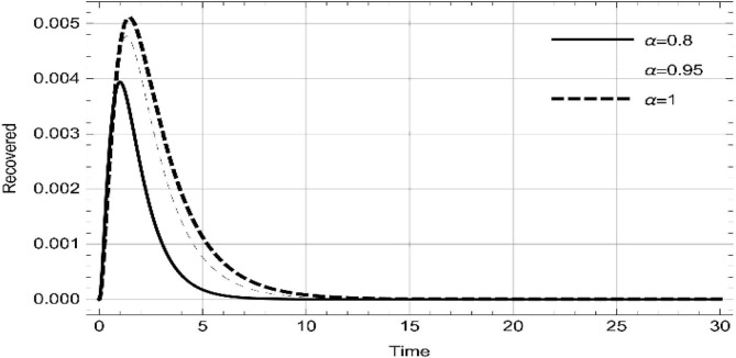
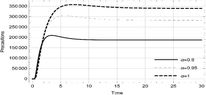
Abstract

In present time, the whole world is in the phase of war against the deadly pandemic COVID'19 and working on different interventions in this regard. Variety of strategies are taken into account from ground level to the state to reduce the transmission rate. For this purpose, the epidemiologists are also augmenting their contribution in structuring such models that could depict a scheme to diminish the basic reproduction number. These tactics also include the awareness campaigns initiated by the stakeholders through digital, print media and etc. Analyzing the cost and profit effectiveness of these tactics, we design an optimal control dynamical model to study the proficiency of each strategy in reducing the virulence of COVID'19. The aim is to illustrate the memory effect on the dynamics of COVID'19 with and without prevention measures through fractional calculus. Therefore, the structure of the model is in line with generalized proportional fractional derivative to assess the effects at each chronological change. Awareness about using medical mask, social distancing, frequent use of sanitizer or cleaning hand and supportive care during treatment are the strategies followed worldwide in this fight. Taking these into consideration, the optimal objective function proposed for the surveillance mitigation of COVID'19, is contemplated as the cost function. The effect analysis is supported through graphs and tabulated values. In addition, sensitivity inspection of basic reproduction number is also carried out with respect to different values of fractional index and cost function. Ultimately, social distancing and supportive care of infected are found to be significant in decreasing the basic reproduction number more rapidly.

Introduction

A deadly coronavirus that basically initiated from Wuhan city of China, all of a sudden incarcerated the people all around the world. This strain of severe acute respiratory syndrome coronavirus 2 (SARS-CoV-2) has affected more than 210 countries and territories. It has brought devastating consequences on public health as well as on social and economic activities. Governments around the world prompted surveillance on mitigating the global spread of COVID'19. Among many of these dramatic measures, majority are substantiating to be effective in reducing the virus transmission. Imposing curfew and locking down the cities in addition public awareness campaigns such as, stay-at-home, encouraging social distancing, cleanliness that include frequent washing hand, using sanitizers through digital and print media are the key measures in restraining this virus. On enforcing these policies and engaging communities in these campaigns, undoubtedly enormous social and economic cost is expected. But until an effectual vaccine or treatment becomes available, these strategies may play important roles [1], [2], [3], [4], [5], [6].

Variety of research has been conducted at an extraordinary pace to analyze the COVID'19 in different perspectives [7], [8], [9]. Epidemiological dynamical systems to control the breakout of this pandemic through basic reproduction number has been obtained by various researchers [10], [11], [12]. Clinical studies to determine therapeutic solutions through the findings of the biological features of this virus [13]. Perceptions on impact of government's preventing strategies on other environmental, social and economic activities [14]. Decision making models to consider an effective managing prevention strategy of COVID'19 transition [15]. Machine learning models to predict the high risk and efficiently triage the patients with high accuracy [16]. Mathematical models fit out to be substantial contrivances in investigating the dynamical controls of the infectious diseases[17]. Research articles, based on optimal control models can be found in the literature to a great extent in this regard [18], [19], [20], [21], [22], [23], [24]. In the recent times of battle against COVID'19, numerous authors have added their valuable contributions in this connection. Grigorieva et al. formulate two SEIR-type model to investigate the cost-effective quarantine strategies and analyzed the optimal solutions numerically [25]. Analysis of interventions of COVID'19 through transmission model and observing the most effective non-pharmaceutical strategies to lessen the disease nuisance in Pakistan is found in the literature [26]. In particular, plenty of endeavors have been carried out in different context of cost-effective strategy, to control the transmission of this deadly pandemic [27], [28].

In this attempt, we design mathematical model that covers two major areas, epidemiology together with dynamical optimal control. Firstly, the compartmental model is taken into account with the control variables and stability analysis are carried out. Secondly, optimizing cost functions is subjected to the compartmental model to assess the cost-effectiveness of the prevention strategies. As aforementioned, there exist significant mathematical efforts in this connection, but the novelties that invigorate the proposed assessment can be classified as:

• •This study is not only susceptible, exposed, quarantine, infected and recovery compartments, but also the isolation and precautions. Thus, the model is named as SEQIMRP i.e. susceptible-expose-quarantined-infected-isolated-recovered-protected.
• •The non-pharmaceutical control variables, awareness campaigns about using mask, encouraging social distancing, signifying frequent use of sanitizer and washing hands, supportive care during treatment.
• •Regulatory of basic reproduction number through these campaigns.
• •Incorporating fractional order derivative for dynamical scrutiny of the model with.

This significant contribution will undoubtedly add great perspicacity of COVID'19 interventions. The proposed SEQIMRP model with proportional fractional [29] signifies the broader application of the fractional definition. Its expansion elegantly converts the fractional order derivative operator into integer order that the fractional order index reallocates linearly in the equations. By virtue of this, the dynamics of COVID’19, for instance the basic reproduction number and equilibrium points can be interpreted with memory effects. Subsequently, historical values of these parameters or the compartmental functions will enable to devise defensive precautionary steps, revealed from the past experiences. In addition, the effect of memory on the optimality of awareness strategies is also illustrated through the proportional fractional derivative. The designed system provides a novel contribution in epidemiological study of epidemic and pandemic diseases. It will instruct the healthcare researchers a new mode of generating results and might be capable to investigating prior information about the risk factors or transmission rate for preparatory measures. The remaining paper contains sections of formulating the dynamical system, stability analysis of equilibrium points and optimality assessment. Furthermore, numerical discussions are also carried out to evidently establish an effective conclusion.

Model formulation for COVID'19 optimal control

Susceptible-expose-quarantined-infected-isolated-recovered-protected (SEQIMRP)

Mathematical models based on disease dynamics are quite helpful in studying the functional behavior of any virus, which then helps to overcome or lessen its contaminating breakout. The destructive coronavirus converted into a pandemic within a few months and affected billions of peoples around a globe. Early laboratory research and scientific experiments to construct a drug or vaccine could not triumph. Many epidemiological models also expressed significant contributions in this connection to determine the basic reproduction number and predict the dispersion, recovery and mortality rates [11], [12], [30]. Here, to analyze the dynamical behavior and impact of COVID'19 pandemic, a system of differential equations is designed with respect to compartmental classes and prevention measures on the basis of following assumptions.

• •Regardless of different risk rate of COVID'19 for different age-group and pre-existing disease carriers, the model assumes a homogeneous mixing of individuals in the population.
• •Prevention strategies: Usage of medical mask $\left(\mathit{mm}\right)$, social distancing $\left(\mathit{sd}\right)$, frequently cleaning hands$\left(\mathit{ch}\right)$ and supportive care$\left(\mathit{sc}\right)$ during treatments are taken into account as control variables of the optimal system.
• •The individuals in any compartment, following the operational prevention strategies, are assumed as will not get infected and are defined by means of protected compartment.
• •Susceptible is outlined in the form of logistic growth that encompasses maximum sustainability to survive in the available resources in an environment.
• •Exposed are quarantined that might recover and use prevention measures later to insulate themselves from virus.
• •Treatment of infected COVID'19 patients is the isolation process, which is explained in the isolation compartment. These compartments with the supportive care from staff might recover and move to recovery compartment.
• •Treated individuals after recovery do not participate in transmitting the disease as they use the operational prevention strategies.
• •The assessments of basic reproduction number and stability analysis are carried out in fractional calculus environment.

Hence, the fractional order epidemiological model, susceptible-expose-quarantined-infected-isolated-recovered-protected (SEQIMRP) is mathematically signified as:

$${}^{PF}D_t^{\alpha }S\left(t\right)=r_{s}S\left(t\right)\left(1-\frac{S\left(t\right)}{k_S}\right)-\left(\mathit{mm}\left(t\right)+sd\left(t\right)+ch\left(t\right)\right)S\left(t\right)-\beta S\left(t\right)I\left(t\right)-d_{s}S\left(t\right)$$

$${}^{PF}D_t^{\alpha }E\left(t\right)=\beta S\left(t\right)I\left(t\right)-\left(\mathit{mm}\left(t\right)+sd\left(t\right)+ch\left(t\right)\right)E\left(t\right)-\gamma E\left(t\right)-d_{E}E\left(t\right)$$

$${}^{PF}D_t^{\alpha }Q\left(t\right)=\gamma E\left(t\right)-\left(\mathit{mm}\left(t\right)+sd\left(t\right)+ch\left(t\right)+sc\left(t\right)\right)Q\left(t\right)-\eta Q\left(t\right)-{\psi }_{Q}Q\left(t\right)-d_{Q}Q\left(t\right)$$ (1)

$${}^{PF}D_t^{\alpha }I\left(t\right)=\eta Q\left(t\right)-\left(\mathit{mm}\left(t\right)+sd\left(t\right)+ch\left(t\right)+sc\left(t\right)\right)I\left(t\right)-\sigma I\left(t\right)-d_{I}I\left(t\right)$$

$${}^{PF}D_t^{\alpha }M\left(t\right)=\sigma I\left(t\right)-\left(\mathit{mm}\left(t\right)+sd\left(t\right)+ch\left(t\right)+sc\left(t\right)\right)M\left(t\right)-{\psi }_{M}M\left(t\right)-\rho M\left(t\right)$$

$${}^{PF}D_t^{\alpha }R\left(t\right)={\psi }_{Q}Q\left(t\right)+{\psi }_{M}M\left(t\right)-\left(\mathit{mm}\left(t\right)+sd\left(t\right)+ch\left(t\right)\right)R\left(t\right)-d_{R}R\left(t\right)$$

$$\begin{array}{c}{}^{PF}D_t^{\alpha }P\left(t\right)=\left(mm\left(t\right)+sd\left(t\right)+ch\left(t\right)\right)\left(S\left(t\right)+E\left(t\right)+R\left(t\right)\right)+\left(mm\left(t\right)+sd\left(t\right)+ch\left(t\right)+sc\left(t\right)\right)Q\left(t\right)\\ +\left(mm\left(t\right)+sd\left(t\right)+ch\left(t\right)+sc\left(t\right)\right)\left(I\left(t\right)+M\left(t\right)\right)-d_{P}P\end{array}$$

with initial conditions,

$$\begin{array}{c}S\left(0\right)=O_1,E\left(0\right)=O_2,Q\left(0\right)=O_3,I\left(0\right)=O_4,\\ M\left(0\right)=O_5,R\left(0\right)=O_6,P\left(0\right)=O_7.\end{array}$$ (2)

where, $O_i\left(0\right)\in {\mathfrak{R}}_{+}^7$ for$i=1,2,\dots ,7$. Table 1 further elaborates the dimensions of all the variables and parameters of system (1). Moreover, pictorial demonstration of the compartmental system, representing the flow of the diseases transmission is also given in Fig. 1 . Assume$\mathrm{N}\left(t\right)$ is the total population density of individuals that can be structured as:

$$\mathrm{N}\left(t\right)=S\left(t\right)+E\left(t\right)+Q\left(t\right)+I\left(t\right)+M\left(t\right)+R\left(t\right)+P\left(t\right)$$ (3)

Table 1.

Variables and parameters of the SEQIMRP.

Compart-mental functions	Descriptions	Units	Initial values(population = in millions & time = days)	Source
$N\left(t\right)$	Total population	Population / day	113	Estimated
$S\left(t\right)$	Susceptible	Population / day	111	Estimated
$E\left(t\right)$	Exposed	Population / day	0	Estimated
$Q\left(t\right)$	Quarantined	Population / day	0	Estimated
$I\left(t\right)$	Infected	Population / day	2	Estimated
$M\left(t\right)$	Infected isolated	Population / day	0	Estimated
$R\left(t\right)$	Recovered	Population / day	0	Estimated
$P\left(t\right)$	Protected	Population / day	0	Estimated
$\alpha$	Order of fractional derivative	Dimensionless	$0<\alpha ⩽1$	Fitted
Parameters	Descriptions	Units	Value	Source
$\xi$	R is taking part in social distancing	Individuals/(individuals × day)	14.771	Fitted
$\beta$	Contact rate of susceptible with infected	Individuals/(individuals × day)	14.781	Fitted
$\gamma$	Rate of exposed individuals quarantined	Individuals/(individuals × day)	1.887 × 10-7	Fitted
$\eta$	Rate of treated infected and quarantined	Individuals/(area × day)	0.13266	Fitted
$\sigma$	Rate of susceptible exposed to quarantine	Individuals/(individuals × day)	0.0714	Fitted
$r_S$	Intrinsic Growth rate of susceptible individuals	Individuals/(individuals × day)	$30$	Fitted
$k_S$	Carrying capacity of susceptible individuals	Individuals/(individuals × day)	100,000	Fitted
$\sigma$	Rate of susceptible exposed to infection	Individuals/(individuals × day)	0.1259	Fitted
$\rho$	Death due to COVID'19 disease	Individuals/(individuals × day)	1.782 × 10-5	[35]
${\psi }_Q$	Recovery rate of the quarantine individuals	Individuals/(individuals × day)	0.11624	Fitted
${\psi }_M$	Recovery rate of the isolated infected individuals	Individuals/(individuals × day)	0.33029	Fitted
$d_S$	Susceptible death rate	Individuals/(individuals × day)	0.15	Fitted
$d_E$	Exposed death rate	Individuals/(individuals × day)	0.84	Fitted
$d_Q$	Quarantined death rate	Individuals/(individuals × day)	0.84	Fitted
$d_I$	Infected death rate	Individuals/(individuals × day)	0.9	Fitted
$d_R$	Recovered death rate	Individuals/(individuals × day)	0.11	Fitted
$d_P$	Precautionary death rate	Individuals/(individuals × day)	0.84	Fitted
$\mathit{mm}$	Rate of individuals using medical mask	Individuals/(individuals × day)	0–1	Fitted
$\mathit{sd}$	Rate of individuals taking part in social distancing	Individuals/(individuals × day)	0–1	Fitted
$\mathit{ch}$	Rate of individuals frequently cleaning hand	Individuals/(individuals × day)	0–1	Fitted
$\mathit{sc}$	Rate of individuals who follow step of supportive care during treatment.	Individuals/(individuals × day)	0–1	Fitted

Fig. 1.

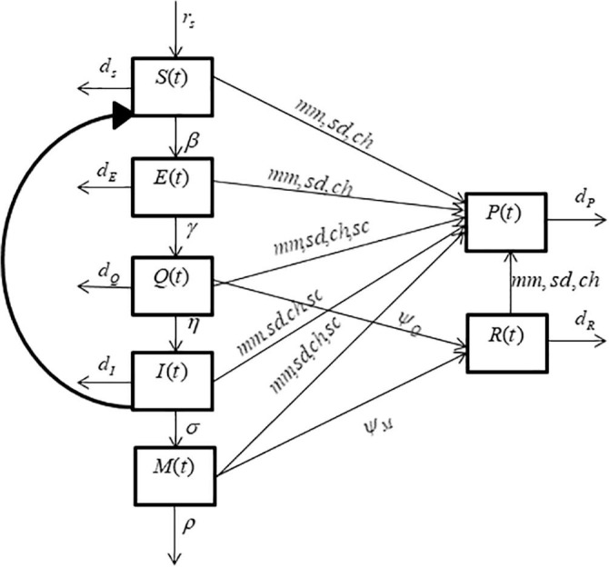
Pictorial illustration of SEQIMRP model.

Moreover, ${}^{\mathit{P}\mathit{F}}D_{\mathit{t}}^{\mathit{\alpha }}$ articulates proportional fractional derivative of order$\alpha \in \left(0,1\right]$ [29], which can be expanded as for any continuous function $y\left(t\right)$,

$${}^{PF}D_t^{\alpha }y\left(t\right)={\ell }_0\left(\alpha ,t\right)\frac{dy\left(t\right)}{\mathit{dt}}+{\ell }_1\left(\alpha ,t\right)y\left(t\right),0<\alpha ⩽1$$ (4)

where, ${\ell }_0\left(\alpha ,t\right)\ne 0$ for $\alpha \in \left(0,1\right]$, with $\underset{\alpha \to 0^{+}}{lim}{\ell }_0\left(\alpha ,t\right)=0$ and $\underset{\alpha \to 1^{-}}{lim}{\ell }_0\left(\alpha ,t\right)=1$. Additionally,${\ell }_1\left(\alpha ,t\right)\ne 0$ for $\alpha \in \left[0,1\right)$, with $\underset{\alpha \to 0^{+}}{lim}{\ell }_1\left(\alpha ,t\right)=1$and$\underset{\alpha \to 1^{-}}{lim}{\ell }_1\left(\alpha ,t\right)=0$. Let, ${\ell }_0\left(\alpha ,t\right)=\alpha$ and${\ell }_1\left(\alpha ,t\right)=1-\alpha$, so Eq. (4) becomes

$${}^{PF}D_t^{\alpha }y\left(t\right)=\alpha \frac{dy\left(t\right)}{\mathit{dt}}+\left(1-\alpha \right)y\left(t\right)$$ (5)

Assume that all control functions (prevention steps) are constant within time, therefore, by applying expansion (5) on system (1), we get the system as:

$$\dot{S}\left(t\right)=\frac{1}{\alpha }\left(r_{s}S\left(t\right)\left(1-\frac{S\left(t\right)}{k_S}\right)-\left(\mathit{mm}+sd+ch\right)S\left(t\right)-\beta S\left(t\right)I\left(t\right)-d_{s}S\left(t\right)-\left(1-\alpha \right)S\left(t\right)\right)$$

$$\dot{E}\left(t\right)=\frac{1}{\alpha }\left(\beta S\left(t\right)I\left(t\right)-\left(\mathit{mm}+sd+ch\right)E\left(t\right)-\gamma E\left(t\right)-d_{E}E\left(t\right)-\left(1-\alpha \right)E\left(t\right)\right)$$

$$\dot{Q}\left(t\right)=\frac{1}{\alpha }\left(\gamma E\left(t\right)-\left(\mathit{mm}+sd+ch+sc\right)Q\left(t\right)-\eta Q\left(t\right)-{\psi }_{Q}Q\left(t\right)-d_{Q}Q\left(t\right)-\left(1-\alpha \right)Q\left(t\right)\right)$$

$$\dot{I}\left(t\right)=\frac{1}{\alpha }\left(\eta Q\left(t\right)-\left(\mathit{mm}+sd+ch+sc\right)I\left(t\right)-\sigma I\left(t\right)-d_{I}I\left(t\right)-\left(1-\alpha \right)I\left(t\right)\right)$$ (6)

$$\dot{M}\left(t\right)=\frac{1}{\alpha }\left(\sigma I\left(t\right)-\left(\mathit{mm}+sd+ch+sc\right)M\left(t\right)-{\psi }_{M}M\left(t\right)-\rho M\left(t\right)-\left(1-\alpha \right)M\left(t\right)\right)$$

$$\dot{R}\left(t\right)=\frac{1}{\alpha }\left({\psi }_{Q}Q\left(t\right)+{\psi }_{M}M\left(t\right)-\left(\mathit{mm}+sd+ch\right)R\left(t\right)-d_{R}R\left(t\right)-\left(1-\alpha \right)R\left(t\right)\right)$$

$$\dot{P}\left(t\right)=\frac{1}{\alpha }\left(\begin{array}{c}\left(\mathit{mm}+sd+ch\right)\left(S\left(t\right)+E\left(t\right)+R\left(t\right)\right)+\left(mm+sd+ch+sc\right)Q\left(t\right)-d_{P}P\\ +\left(\mathit{mm}+sd+ch+sc\right)\left(I\left(t\right)+M\left(t\right)\right)-\left(1-\alpha \right)P\left(t\right)\end{array}\right)$$

with the same initial conditions (2). System (6) evidently depicts the lucidity of the proportional fractional derivative, which greatly reduces the manipulation complexities of system (1).

Theorem 1 (Boundedness) —

Let $\mathrm{\Pi }\in {\mathfrak{R}}_{+}^7$ is the set of all feasible solutions of the system (6), then there exists uniformly bounded subset of ${\mathfrak{R}}_{+}^7$ such that:

$$\mathrm{\Pi }=\left\{\left(S,E,Q,I,M,R,P\right)\in {\mathfrak{R}}_{+}^7;\mathrm{N}\left(t\right)⩽\frac{r_S}{d_{\mathrm{N}}^{\ast }{k}_S}\right\}$$ (7)

Proof:

By applying proportional fractional derivative and its expansion, as defined in the Eqs. (4)-(5), on Eq. (3), we get the expression of the form:

$$\mathrm{N}\left(t\right)=\frac{1}{\alpha }\left(\dot{S}\left(t\right)+\dot{E}\left(t\right)+\dot{Q}\left(t\right)+\dot{I}\left(t\right)+\dot{M}\left(t\right)+\dot{R}\left(t\right)+\dot{P}\left(t\right)-\left(1-\alpha \right)\mathrm{N}\left(t\right)\right)$$ (8)

On simplifying by using system (6) and suppose $d_{\mathrm{N}}^{\ast }$ be total proportion of deaths in all compartments i.e.

$$d_{\mathrm{N}}^{\ast }\mathrm{N}\left(t\right)=d_{S}S\left(t\right)+d_{E}E\left(t\right)+d_{Q}Q\left(t\right)+d_{I}I\left(t\right)+d_{R}R\left(t\right)+\rho M\left(t\right)+d_{P}P\left(t\right)$$ (9)

In addition, since$0<\alpha ⩽1$

$$\dot{\mathrm{N}}\left(t\right)⩽r_{S}S\left(t\right)\left(1-\frac{S\left(t\right)}{k_S}\right)-d_{\mathrm{N}}^{\ast }\mathrm{N}\left(t\right)$$ (10)

where $0<\frac{S\left(t\right)}{k_S}⩽1$, so the above inequality reduces to

$$\dot{\mathrm{N}}\left(t\right)⩽\frac{r_S}{k_S}-d_{\mathrm{N}}^{\ast }\mathrm{N}\left(t\right)$$ (11)

On integrating

$$\mathrm{N}\left(t\right)⩽e^{-t{d}_{\mathrm{N}}^{\ast }}\mathrm{N}\left(0\right)+\frac{r_S}{d_{\mathrm{N}}^{\ast }{k}_S}$$ (12)

Therefore as $t\to \infty$ , we obtained the final statement of boundedness as

$$\mathrm{N}\left(t\right)⩽\frac{r_S}{d_{\mathrm{N}}^{\ast }{k}_S}$$ (13)

Theorem 2 (Existence and Uniqueness) —

Assume the matrix of right hand side of system (6) be the real-valued function $\mathbf{\Lambda }\left(\mathit{F}\left(t\right)\right):{\mathfrak{R}}_{+}^7\to {\mathfrak{R}}_{+}^7$, such that $\mathbf{\Lambda }\left(\mathit{F}\left(t\right)\right)$ and $\frac{\partial \mathbf{\Lambda }\left(\mathit{F}\left(t\right)\right)}{\partial \mathit{F}\left(t\right)}$ are continuous and

$$∥\mathbf{\Lambda }\left(\mathit{F}\left(t\right)\right)∥⩽\left(\frac{\mathrm{X}}{\left|\alpha \right|}-\nu \right)∥\mathit{F}\left(t\right)∥,\forall \mathit{F}\left(t\right)\in {\mathfrak{R}}_{+}^{7}and0<\alpha ⩽1$$ (14)

Then, satisfying the initial conditions (2), there exists a unique, non-negative and bounded solution of the system (6).

Proof:

Boundedness of system (6) can be followed from Theorem 1, now assume, the system (6) can be expressed as:

$$\dot{\mathit{F}}\left(t\right)=\mathbf{\Lambda }\left(\mathit{F}\left(t\right)\right)$$

where,

$$\mathit{F}\left(t\right)={\left[\begin{array}{ccccccc}S\left(t\right)& E\left(t\right)& Q\left(t\right)& I\left(t\right)& M\left(t\right)& R\left(t\right)& P\left(t\right)\end{array}\right]}^T$$ (15)

and

$$\mathbf{\Lambda }\left(\mathit{F}\left(t\right)\right)=\frac{1}{\alpha }\left[\begin{array}{c}{r}_{s}S\left(t\right)\left(1-\frac{S\left(t\right)}{k_S}\right)-\left(\mathit{mm}+sd+ch\right)S\left(t\right)-\beta S\left(t\right)I\left(t\right)-d_{s}S\left(t\right)-\left(1-\alpha \right)S\left(t\right)\\ \beta S\left(t\right)I\left(t\right)-\left(\mathit{mm}+sd+ch\right)E\left(t\right)-\gamma E\left(t\right)-d_{E}E\left(t\right)-\left(1-\alpha \right)E\left(t\right)\\ \gamma E\left(t\right)-\left(\mathit{mm}+sd+ch+sc\right)Q\left(t\right)-\eta Q\left(t\right)-{\psi }_{Q}Q\left(t\right)-d_{Q}Q\left(t\right)-\left(1-\alpha \right)Q\left(t\right)\\ \eta Q\left(t\right)-\left(\mathit{mm}+sd+ch+sc\right)I\left(t\right)-\sigma I\left(t\right)-d_{I}I\left(t\right)-\left(1-\alpha \right)I\left(t\right)\\ \sigma I\left(t\right)-\left(\mathit{mm}+sd+ch+sc\right)M\left(t\right)-{\psi }_{M}M\left(t\right)-\rho M\left(t\right)-\left(1-\alpha \right)M\left(t\right)\\ {\psi }_{Q}Q\left(t\right)+{\psi }_{M}M\left(t\right)-\left(\mathit{mm}+sd+ch\right)R\left(t\right)-d_{R}R\left(t\right)-\left(1-\alpha \right)R\left(t\right)\\ \left(\mathit{mm}+sd+ch\right)\left(S\left(t\right)+E\left(t\right)+R\left(t\right)\right)+\left(\mathit{mm}+sd+ch+sc\right)\left(Q\left(t\right)+I\left(t\right)+M\left(t\right)\right)\\ -d_{P}P-\left(1-\alpha \right)P\left(t\right)\end{array}\right]$$ (16)

Eq. (16) can be further expanded into:

$$\mathbf{\Lambda }\left(\mathit{F}\left(t\right)\right)=\frac{1}{\alpha }\left({\mathrm{\Omega }}_1\mathit{F}\left(t\right)+S\left(t\right){\mathrm{\Omega }}_2\mathit{F}\left(t\right)+I\left(t\right){\mathrm{\Omega }}_3\mathit{F}\left(t\right)-\left(\alpha -1\right)\mathit{F}\left(t\right)\right)$$ (17)

such that

$${\mathrm{\Omega }}_1={\left[\begin{array}{ccccccc}{r}_S-M_1-d_S& 0& 0& 0& 0& 0& 0\\ 0& -M_1-\gamma -d_E& 0& 0& 0& 0& 0\\ 0& 0& -M_2-\eta -{\psi }_Q-d_Q& 0& 0& 0& 0\\ 0& 0& \eta & -M_2-\sigma -d_I& 0& 0& 0\\ 0& 0& 0& \sigma & -M_2-{\psi }_M-\rho & 0& 0\\ 0& 0& {\psi }_Q& 0& {\psi }_M& -M_1-d_R& 0\\ M_1& M_1& M_2& M_2& M_2& M_1& -d_P\end{array}\right]}_{7\times 7}$$

$$M_1=mm+sd+ch$$

$$M_2=mm+sd+ch+sc$$

${\mathrm{\Omega }}_2={\left[-\begin{array}{cc}{r}_S/k_S& \mathbf{0}\end{array}\right]}_{1\times 7}$ and ${\mathrm{\Omega }}_3={\left[\begin{array}{cccc}-\beta & 0& \beta & \mathbf{0}\end{array}\right]}_{1\times 7}$. Then, Eq. (17) can be rewritten as,

$$\begin{array}{c}∥\mathbf{\Lambda }\left(\mathit{F}\left(t\right)\right)∥=∥\frac{1}{\alpha }\left({\mathrm{\Omega }}_1\mathit{F}\left(t\right)+S\left(t\right){\mathrm{\Omega }}_2\mathit{F}\left(t\right)+I\left(t\right){\mathrm{\Omega }}_3\mathit{F}\left(t\right)-\left(\alpha -1\right)\mathit{F}\left(t\right)\right)∥\\ ⩽\left|\frac{1}{\alpha }\right|\left(\left(∥{\mathrm{\Omega }}_1∥+∥{\mathrm{\Omega }}_2∥+∥{\mathrm{\Omega }}_3∥+\left|\left(\alpha -1\right)\right|\right)∥\mathit{F}\left(t\right)∥\right)\end{array}$$

Let $\mathrm{X}=∥{\mathrm{\Omega }}_1∥+∥{\mathrm{\Omega }}_2∥+∥{\mathrm{\Omega }}_3∥$, so the final statement is achieved as for $0<\alpha ⩽1$ ,

$$∥\mathbf{\Lambda }\left(\mathit{F}\left(t\right)\right)∥⩽\left(\frac{\mathrm{X}}{\left|\alpha \right|}-\nu \right)∥\mathit{F}\left(t\right)∥$$

where $\nu =\left|\left(\frac{1}{\alpha }-1\right)\right|$. Next, we prove the non-negativity of the solutions by using the positivity of initial conditions (2) i.e.,$O_i>0$ for $i=1,2,\dots ,7$. Considering first equation of system (6), it can be deduced to:

$$\begin{array}{c}\dot{S}\left(t\right)=\frac{1}{\alpha }\left(r_{s}S\left(t\right)\left(1-\frac{S\left(t\right)}{k_S}\right)-\left(\mathit{mm}+sd+ch\right)S\left(t\right)-\beta S\left(t\right)I\left(t\right)-d_{s}S\left(t\right)-\left(1-\alpha \right)S\left(t\right)\right)\\ ⩾-\frac{1}{\alpha }\left(\mathit{mm}+sd+ch+d_S+\left(1-\alpha \right)\right)S\left(t\right)\end{array}$$

On manipulating, we get

$$S\left(t\right)⩾O_1{e}^{-\left(\left(\mathit{mm}+sd+ch+d_S+\left(1-\alpha \right)\right)/\alpha \right)t}$$ (18)

Since $0⩽e^{-\left(\left(\mathit{mm}+sd+ch+d_S+\left(1-\alpha \right)\right)/\alpha \right)t}⩽1$ for $t>0$, therefore Eq. (18) reduces to,

$$S\left(t\right)⩾0$$

Thus, proved the non-negativity of $S\left(t\right)$. Analogously, all the remaining equations of system (6) can be proved to have non-negative solutions with the assumption of positive initial conditions.

Optimal control problem

Furthermore, the dynamical model (6) of COVID'19 would be incomplete if the assumption of optimal control of infection and intervention cost is not incorporated. Therefore, we formulate optimal control problem by means of the cost function type of quadratic function as:

$$J\left(Y_i,{\mathit{U}}_k\right)={\int }_0^{t_f}\left(\sum _{i=1}^7{w}_i{Y}_i^2+{\phi }_{1}m{m}^2+{\phi }_{2}s{d}^2+{\phi }_{3}c{h}^2+{\phi }_{4}s{c}^2\right)dt$$ (19)

where,$\forall Y_i⩾0$ for $i=1,2,...7$are replace by $S,E,Q,I,M,R,P,$respectively. Moreover, here $w_i$ , for $i=1,2,...,7$, are the weights of human population cost, whereas ${\phi }_K$ , for $K=1,2,3,4$, are the weights of undertaken intervention cost for COVID'19. At this juncture, intervention cost comes from government campaigns of using mask, social distancing and frequently washing hand. In addition, the hospitalization cost for drugs, ventilators and trained medical staffs for supportive care of the COVID'19 infected individuals also become higher with the increase in number of patients. Therefore, if greater cost is implemented of campaigns of enforcing the people on usage of mask, social distancing and frequently washing hand will reduce the COVID'19 transmission, which on the other hand it reduces the supportive care cost. Thus, we assume ${\phi }_K>0$ , for $K=1,2,3,4$. Analogously, the objective of the present scenario is to control the spread out of COVID'19, which ultimately leads to minimize the infected individuals, therefore we consider $w_4>0$and remaining equal to zero.

Basic reproduction number $R_0$

In this sequel, we utilize the next generation method, to structure the $R_0$ for the governing model (6). For this purpose, a sub-model of the SEQIMRP is considered that includes the four infected classes i.e. exposed, quarantine, infected and isolated individuals. Therefore, the equation:

$$\frac{d\overrightarrow{\mathit{X}}}{\mathit{dt}}=\mathrm{F}\left(\overrightarrow{\mathbf{X}}\right)-\mathrm{V}\left(\overrightarrow{\mathbf{X}}\right)$$ (20)

will have $\overrightarrow{\mathit{X}}$ as a vector of the$E\left(t\right)$,$Q\left(t\right)$, $I\left(t\right),$ and $M\left(t\right)$, which is outlined as,

$$\overrightarrow{\mathit{X}}={\left[\begin{array}{ccc}E& Q& IM\end{array}\right]}^t$$

with, $\mathrm{F}\left(\overrightarrow{\mathbf{X}}\right)$ expressed as,

$$\mathrm{F}\left(\overrightarrow{\mathbf{X}}\right)={\left[\begin{array}{ccc}\beta \mathrm{S}\mathrm{I}/\alpha & 0& 0\end{array}0\right]}^{\mathrm{t}}$$

On the other hand,$\mathrm{V}\left(\overrightarrow{\mathbf{X}}\right)$, can be further split down as,

$$\mathrm{V}\left(\overrightarrow{\mathbf{X}}\right)=\left[\begin{array}{c}\left(mm+sd+ch+\gamma +d_E+\left(1-\alpha \right)\right)E\left(\mathit{t}\right)/\alpha \\ \begin{array}{c}\left(mm+sd+ch+sc+\eta +{\psi }_Q+d_Q+\left(1-\alpha \right)\right)Q\left(\mathit{t}\right)/\alpha \\ \left(mm+sd+ch+sc+\sigma +d_I+\left(1-\alpha \right)\right)I\left(\mathit{t}\right)/\alpha \end{array}\\ \left(mm+sd+ch+sc+{\psi }_M+\rho +\left(1-\alpha \right)\right)M\left(\mathit{t}\right)/\alpha \end{array}\right]-\left[\begin{array}{c}\begin{array}{c}0\\ \gamma E\left(\mathit{t}\right)/\alpha \end{array}\\ \eta Q\left(\mathit{t}\right)/\alpha \\ \sigma I\left(\mathit{t}\right)/\alpha \end{array}\right]$$

Taking Jacobian matrix of Eq. (20) at disease free equilibrium point,${\mathrm{\Pi }}_1\left(-k_S\left(1+d_S-r_S+mm+sd+ch-\alpha \right)/r_S,0,0,0,0,0,0\right)$, we get,

$$\mathit{J}\left[\frac{d\overrightarrow{\mathbf{X}}}{dt}\right]=\mathbf{F}\mathbf{-}\mathbf{V}=\left(\begin{array}{cccc}0& 0& {\mathrm{H}}_{13}& 0\\ 0& 0& 0& 0\\ 0& 0& 0& 0\\ 0& 0& 0& 0\end{array}\right)-\left(\begin{array}{cccc}{\mathrm{\Delta }}_{11}& 0& 0& 0\\ {\mathrm{\Delta }}_{21}& {\mathrm{\Delta }}_{22}& 0& 0\\ 0& {\mathrm{\Delta }}_{32}& {\mathrm{\Delta }}_{33}& 0\\ 0& 0& {\mathrm{\Delta }}_{43}& {\mathrm{\Delta }}_{44}\end{array}\right)$$ (21)

where,

${\mathrm{H}}_{13}=$ $-\beta k{}_S\left(1+d_S-r_S+mm+sd+ch-\alpha \right)/\alpha r_S$

${\mathrm{\Delta }}_{11}=\left(\mathit{mm}+sd+ch+\gamma +d_E+\left(1-\alpha \right)\right)/\alpha$

${\mathrm{\Delta }}_{21}=-\gamma /\alpha$, ${\mathrm{\Delta }}_{22}=\left(\mathit{mm}+sd+ch+sc+\eta +{\psi }_Q+d_Q+\left(1-\alpha \right)\right)/\alpha$,

${\mathrm{\Delta }}_{32}=-\eta /\alpha ,$ ${\mathrm{\Delta }}_{33}=\left(\mathit{mm}+sd+ch+sc+\sigma +d_I+\left(1-\alpha \right)\right)/\alpha ,$

${\mathrm{\Delta }}_{43}=-\sigma /\alpha ,$ ${\mathrm{\Delta }}_{44}=\left(\mathit{mm}+sd+ch+sc+{\psi }_M+\rho +\left(1-\alpha \right)\right)/\alpha$

From Eq. (21), we can extract and manipulate,

$$\mathbf{K}=\mathbf{F}{\mathbf{V}}^{-1}$$

The spectral radius $\mathrm{\Lambda }\left(\mathbf{K}\right)$ is the required basic reproduction number, so after some simplification we get

$$\begin{array}{c}{R}_0=-k_S\beta \gamma \eta \left(1+d_S-r_S+mm+sd+ch-\alpha \right)/r{}_S\left(1+d_E+mm+sd+ch-\alpha +\gamma \right)\\ \left(1+d_I+mm+sd+ch+sc-\alpha +\sigma \right)\left(1+d_Q+mm+sd+ch+sc-\alpha +\eta +{\psi }_Q\right)\end{array}$$ (22)

Consequently, the generated $R_0$ contains the fractional derivative index $\alpha$ as well, which advantageously enables to inspect $R_0$. The health care researchers will be capable to investigate the trajectory of basic reproduction number for the COVID'19 at small change.

Dynamical anatomization

In this section, on the strength of proportional fractional derivative, dynamical analysis of equilibrium points and optimality conditions are discussed in fractional environment as follows:

Systematic stability analysis

Theorem 3 (Trivial Equilibrium Point) —

The trivial equilibrium solution, ${\mathrm{\Pi }}_0\left(0,0,0,0,0,0,0\right)\in {\mathfrak{R}}_{+}^7$, of system (6), is asymptotically unstable, for $0<\alpha ⩽1$.

Proof:

It can be easily proved by eigenvalues of $\mathit{J}$ at ${\mathrm{\Pi }}_0\left(0,0,0,0,0,0,0\right)\in {\mathfrak{R}}_{+}^7$, for all $0<\alpha ⩽1$,

${\lambda }_1=\frac{-1-d_P+\alpha }{\alpha }$,${\lambda }_2=\frac{-1-d_R-mm-sd-ch+\alpha }{\alpha }$,${\lambda }_3=\frac{-1-d_S+r_S-mm-sd-ch+\alpha }{\alpha }$,${\lambda }_4=\frac{-1-d_E-mm-sd-ch+\alpha -\gamma }{\alpha }$,

${\lambda }_5=\frac{-1-d_I-mm-sd-ch-sc+\alpha -\sigma }{\alpha }$,${\lambda }_6=\frac{-1-mm-sd-ch-sc+\alpha -\rho -{\psi }_M}{\alpha }$ , ${\lambda }_7=\frac{-1-d_Q-mm-sd-ch-sc+\alpha -\eta -{\psi }_Q}{\alpha }$.

Since$r_S>1+d_S+mm+sd+ch-\alpha$, it is clear that${\lambda }_3>0$, for$0<\alpha ⩽1$. Thus, ${\mathrm{\Pi }}_0\in {\mathfrak{R}}_{+}^7$ is unstable.

Theorem 4 (Disease Free Equilibrium Point) —

The disease-free equilibrium of the system (6)

$${\mathrm{\Pi }}_1\left(-k_S\left(1+d_S-r_S+mm+sd+ch-\alpha \right)/r_S,0,0,0,0,0,0\right)\in {\mathfrak{R}}_{+}^7$$

For $r_S>1+d_S+mm+sd+ch-\alpha$, is locally asymptotically stable if $R_0<1$ and unstable when $R_0>1$, for $0⩽\alpha <1$.

Proof:

On manipulating Jacobian at ${\mathrm{\Pi }}_1\left(-k_S\left(1+d_S-r_S+mm+sd+ch-\alpha \right)/r_S,0,0,0,0,0,0\right)\in {\mathfrak{R}}_{+}^7$, the negative eigenvalues i.e. ${\lambda }_i\in {\mathfrak{R}}_{-}^7$ for $i=1,2,3,4$, are attained as:

${\lambda }_1=\frac{1+d_S-r_S+mm+sd+ch-\alpha }{\alpha }$,${\lambda }_2=\frac{-1-d_P+\alpha }{\alpha }$,${\lambda }_3=\frac{-1-d_R-mm-sd-ch+\alpha }{\alpha }$,${\lambda }_4=\frac{-1-mm-sd-ch-sc+\alpha -\rho -{\psi }_M}{\alpha }$,

with the equation,

$$P\left(\lambda \right)={\lambda }^3+b_2{\lambda }^2+b_1\lambda +b_0\left(1-R_0\right)=0$$ (23)

where

$$b_2=\frac{1}{\alpha }\left(3+d_E+d_I+d_Q+3mm+3sd+3ch+2sc-3\alpha +\gamma +\eta +\sigma +{\psi }_Q\right),$$

$$\begin{array}{l}{b}_1=\frac{1}{{\alpha }^2}\left(\begin{array}{c}3+2d_Q+6mm+2mm{d}_Q+3m{m}^2+6sd+2sd{d}_Q+6mmsd+3s{d}^2\\ +6ch+2ch{d}_Q+6mmch+6sdch+3c{h}^2+4sc+sc{d}_Q+4mmsc+4sdsc\\ +4chsc+s{c}^2-\alpha \left(6+2d_Q+6mm+6sd+6ch+4sc-3\alpha \right)\\ +\gamma \left(2+d_Q+2mm+2sd+2ch+2sc-2\alpha \right)\\ +\eta \left(2+2mm+2sd+2ch+2sc-2\alpha +\gamma \right)\\ +\sigma \left(2+d_Q+2mm+2sd+2ch+sc-2\alpha +\gamma +\eta \right)\\ +\left(2+2mm+2sd+2ch+sc-2\alpha +\gamma +\sigma \right){\psi }_Q\\ +d_I\left(2+d_Q+2mm+2sd+2ch+sc-2\alpha +\gamma +\eta +{\psi }_Q\right)\\ +d_E\left(2+d_I+d_Q+2mm+2sd+2ch+2sc-2\alpha +\eta +\sigma +{\psi }_Q\right)\end{array}\right),\\ b_0=\frac{Z}{{\alpha }^3}\end{array}$$

where

$$\begin{array}{c}Z=\left(1+d_E+mm+sd+ch-\alpha +\gamma \right)\left(1+d_I+mm+sd+ch+sc-\alpha +\sigma \right)\\ \left(1+d_Q+mm+sd+ch+sc-\alpha +\eta +{\psi }_Q\right)\end{array}$$

On applying Routh-Hurwitz criteria [31], [32], [33], [34] i.e. if $b_2>0$, $b_0\left(1-R_0\right)>0$ and $b_1{b}_2>b_0\left(1-R_0\right),$then polynomial (23) is greater than zero and thus all the real part of the eigenvalues must be negative. It can be evidently seen that $b_i>0$for $i=0,1,2$, now the thing which left to prove is $\left(1-R_0\right)>0$. Hence, ${\mathrm{\Pi }}_1\in {\mathfrak{R}}_{+}^7$is locally asymptotically stable if $R_0<1$ and if $R_0>1$, $\left(1-R_0\right)<0$ implies$P\left(\lambda \right)<0$ that is Eq. (23) must have a nonnegative real part, thus ${\mathrm{\Pi }}_1\in {\mathfrak{R}}_{+}^7$ becomes unstable.

Theorem 5 (Endemic Equilibrium Point) —

The endemic equilibrium ${\mathrm{\Pi }}_2\left(\widehat{S},\widehat{E},\widehat{Q},\widehat{I},\widehat{M},\widehat{R},\widehat{P}\right)\in {\mathfrak{R}}_{+}^7$ is locally asymptotically stable if and only if, $R_0>1$ , for $0⩽\alpha <1$.

Proof:

The Jacobian at ${\mathrm{\Pi }}_2\left(\widehat{S},\widehat{E},\widehat{Q},\widehat{I},\widehat{M},\widehat{R},\widehat{P}\right)\in {\mathfrak{R}}_{+}^7$, generates the negative real eigenvalues,

$${\lambda }_1=\frac{-1-d_P+\alpha }{\alpha }{\lambda }_2=\frac{-1-d_R-mm-sd-ch+\alpha }{\alpha }{\lambda }_3=\frac{-1-mm-sd-ch-sc+\alpha -\rho -{\psi }_M}{\alpha }$$

with the polynomial equation,

$$D\left(\lambda \right)={\lambda }^4+K_3{\lambda }^3+K_2{\lambda }^2+K_1\lambda +K_0=0$$ (24)

where,

$$K_3=\frac{-\left(1+d_S-r_S+mm+sd+ch-\alpha \right)}{\alpha R_0}+b_2$$

$$K_2=\left(K_3-b_2\right)b_2+\frac{B}{{\alpha }^2}$$

$$K_1=\left(\frac{B\left(K_3-b_2\right)}{{\alpha }^2}\right)$$

$$K_0=\frac{\left(1+d_S-r_S+mm+sd+ch-\alpha \right)}{{\alpha }^4{R}_0}\left(\frac{k_S\left(1+d_S-r_S+mm+sd+ch-\alpha \right)\beta \gamma \eta }{r_S}+A\right)$$

where,

$$\begin{array}{c}A=1+d_Q+3mm+2d_{Q}mm+3m{m}^2+d_{Q}m{m}^2+m{m}^3+3sd+2d_{Q}sd+6mmsd\\ +2d_{Q}mmsd+3m{m}^{2}sd+3s{d}^2+d_{Q}s{d}^2+3mms{d}^2+s{d}^3+3ch+2d_{Q}ch\\ +6mmch+2d_{Q}mmch+3m{m}^{2}ch+6sdch+2d_{Q}sdch+6mmsdch\\ +3s{d}^{2}ch+3c{h}^2+d_{Q}c{h}^2+3mmc{h}^2+3sdc{h}^2+c{h}^3+2sc+d_{Q}sc\\ +4mmsc+d_{Q}mmsc+2m{m}^{2}sc+4sdsc+d_{Q}sdsc+4mmsdsc+2s{d}^{2}sc\\ +4chsc+d_{Q}chsc+4mmchsc+4sdchsc+24c{h}^{2}sc+s{c}^2+mms{c}^2+sds{c}^2+chs{c}^2\\ -\alpha \left(\begin{array}{c}3+2d_Q+6mm+2d_{Q}mm+3m{m}^2+6sd+2d_{Q}sd+6mmsd+3s{d}^2+6ch+2d_{Q}ch\\ +6mmch+6sdch+3c{h}^2+4sc+d_{Q}sc+4mmsc+4sdsc+4chsc\\ +s{c}^2-3\alpha -d_Q\alpha -3mm\alpha -3sd\alpha -3ch\alpha -2sc\alpha -{\alpha }^2\end{array}\right)\\ +\gamma \left(\begin{array}{c}1+d_Q+2mm+d_{Q}mm+m{m}^2+2sd+d_{Q}sd+2mmsd+s{d}^2+2ch\\ +d_Q{u}_{3}ch+2mmch+2sdch+c{h}^2+2sc+d_{Q}sc+2mmsc+2sdsc\\ +2chsc+s{c}^2-2\alpha -2mm\alpha -2sd\alpha -2ch\alpha -2sc\alpha +{\alpha }^2\end{array}\right)\\ +\eta \left(\begin{array}{c}1+2mm+m{m}^2+2sd+2mmsd+s{d}^2+2ch+2mmch+2sdch+s{d}^2+sc\\ +mmsc+sdsc+chsc-2\alpha -2mm\alpha -2sd\alpha -2ch\alpha -sc\alpha +{\alpha }^2\end{array}\right)\\ +\sigma \left(\begin{array}{c}1+d_Q+2mm+d_{Q}mm+m{m}^2+2sd+d_{Q}sd+2mmsd+s{d}^2\\ +2ch+d_{Q}ch+2mmch+2sdch+c{h}^2+sc+mmsc+sdsc\\ +chsc-2\alpha -d_Q\alpha -2mm\alpha -2sd\alpha -2ch\alpha -sc\alpha +a^2\end{array}\right)\\ +\gamma \sigma \left(1+d_Q+mm+sd+ch+sc-\alpha \right)+\eta \sigma \left(1+mm+sd+ch-\alpha +\gamma \right)\\ +\left(1+mm+sd+ch-\alpha +\gamma \right)\left(1+mm+sd+ch+sc-\alpha +\sigma \right){\psi }_Q+\gamma \eta \left(1+mm+sd+ch+sc-\alpha -k_S\beta \right)\\ +d_I\left(1+mm+sd+ch-\alpha +\gamma \right)\left(1+d_Q+mm+sd+ch+sc-\alpha +\eta +{\psi }_Q\right)\\ +d_E\left(1+d_I+mm+sd+ch+sc-\alpha +\sigma \right)\left(1+d_Q+mm+sd+ch+sc-\alpha +\eta +{\psi }_Q\right)\end{array}$$

and

$$\begin{array}{c}B=3+2d_Q+6mm+2d_{Q}mm+3m{m}^2+6sd+2d_{Q}sd+6mmsd+3s{d}^2+6ch\\ +2d_{Q}ch+6mmch+6sdch+3c{h}^2+4sc++d_{Q}sc+4mmsc\\ +4sdsc+4scch+s{c}^2-6\alpha -2d_Q\alpha -6mm\alpha -6sd\alpha -6ch\alpha \\ -4sc\alpha +3{\alpha }^2+2\gamma +d_Q\gamma +2mm\gamma +2sd\gamma +2ch\gamma +2sc\gamma \\ -2\alpha \gamma +2\eta +2mm\eta +2sd\eta +2ch\eta +sc\eta -2\alpha \eta +\gamma \eta +2\sigma +d_Q\sigma \\ +2mm\sigma +2sd\sigma +2ch\sigma +sc\sigma -2\alpha \sigma +\gamma \sigma +\eta \sigma +\left(2+2mm+2sd+2ch+sc-2\alpha +\gamma +\sigma \right){\psi }_Q\\ +d_I\left(2+d_Q+2mm+2sd+2ch+sc-2\alpha +\gamma +\eta +{\psi }_Q\right)\\ +\left(2+d_I+d_Q+2mm+2sd+2ch+2sc-2\alpha +\eta +\sigma +{\psi }_Q\right).\end{array}$$

The factor $\left(\frac{k_S\left(1+d_S-r_S+mm+sd+ch-\alpha \right)\beta \gamma \eta }{r_S}+A\right)<0$, if the magnitude of $\frac{k_S\left(1+d_S-r_S+mm+sd+ch-\alpha \right)\beta \gamma \eta }{r_S}>A$, which implies that $K_0$ becomes positive if and only if $R_0>1$. Thus with reference to Lemma 5.1 of [20], the positive constant of the polynomial $D\left(\lambda \right)$ implies ${\mathrm{\Pi }}_2\left(\widehat{S},\widehat{E},\widehat{Q},\widehat{I},\widehat{M},\widehat{R},\widehat{P}\right)\in {\mathfrak{R}}_{+}^7$ is locally asymptotically stable if $R_0>1$.

Characterization of optimal control

It is evidently clear from Theorem 1 that there exist a unique solution of system (6). Now to optimize the solution, we define the Lagrangian by

$$L\left(Y_i\right)=\sum _{i=1}^7{w}_i{Y}_i^2+{\phi }_{1}m{m}^2+{\phi }_{2}s{d}^2+{\phi }_{3}c{h}^2+{\phi }_{4}s{c}^2$$ (25)

In addition, describing the Hamiltonian $H$as the inner product of the right hand side of the state system (6) and the adjoint variables $\mathrm{\Omega }=\left({\omega }_1,{\omega }_2,{\omega }_3,{\omega }_4,{\omega }_5,{\omega }_6,{\omega }_7\right)$, we get

$$\begin{array}{c}\mathrm{H}\left(S,E,Q,I,M,R,P,\mathrm{\Omega },t\right)=L\left(Y_i\right)+{\omega }_1\left(t\right)\dot{S}\left(t\right)+{\omega }_2\left(t\right)\dot{E}\left(t\right)+{\omega }_3\left(t\right)\dot{Q}\left(t\right)+{\omega }_4\left(t\right)\dot{I}\left(t\right)\\ +{\omega }_5\left(t\right)\dot{M}\left(t\right)+{\omega }_6\left(t\right)\dot{R}\left(t\right)+{\omega }_7\left(t\right)\dot{P}\left(t\right)\end{array}$$ (26)

where $\mathrm{\Omega }$ is to be determined. Now, utilizing the Pontryagin’s maximum principle for the Hamiltonian $H$, following theorem is obtained to determine the adjoint variables.

Theorem 6 (Existence of adjoint variable) —

For the controlling functions $m{m}^{*}$, $s{d}^{\ast }$, $c{h}^{*}$ and $s{c}^{\ast }$ together with the solution $\left(S^{\ast }\left(t\right),E^{\ast }\left(t\right),I^{\ast }\left(t\right),Q^{\ast }\left(t\right),M^{\ast }\left(t\right),R^{\ast }\left(t\right),P^{\ast }\left(t\right)\right)$ of the corresponding system (6), there exists adjoint variables $\mathrm{\Omega }=\left({\omega }_1,{\omega }_2,{\omega }_3,{\omega }_4,{\omega }_5,{\omega }_6,{\omega }_7\right)$ that satisfy,

$$\begin{array}{c}\frac{d{\omega }_1\left(t\right)}{\mathit{dt}}=\frac{-\left(-1-d_S-\frac{r_{S}S\ast \left(t\right)}{k_S}+r_S\left(1-\frac{S\ast \left(t\right)}{k_S}\right)-mm-sd-ch+\alpha -I\ast \left(t\right)\beta \right){\omega }_1\left(t\right)}{\alpha }\\ -\frac{I\ast \left(t\right)\beta {\omega }_2\left(t\right)}{\alpha }-\frac{\left(\mathit{mm}+sd+ch\right){\omega }_7\left(t\right)}{\alpha }\end{array}$$

$$\frac{d{\omega }_2\left(t\right)}{\mathit{dt}}=\frac{-\left(-1-d_E-mm-sd-ch+\alpha -\gamma \right){\omega }_2\left(t\right)}{\alpha }-\frac{\gamma {\omega }_3\left(t\right)}{\alpha }-\frac{\left(\mathit{mm}+sd+ch\right){\omega }_7\left(t\right)}{\alpha }$$

$$\begin{array}{c}\frac{d{\omega }_3\left(t\right)}{\mathit{dt}}=\frac{-\left(-1-d_Q-mm-sd-ch-sc+\alpha -\eta -{\psi }_Q\right){\omega }_3\left(t\right)}{\alpha }\\ -\frac{\eta {\omega }_4\left(t\right)}{\alpha }-\frac{{\psi }_Q{\omega }_6\left(t\right)}{\alpha }-\frac{\left(\mathit{mm}+sd+ch+sc\right){\omega }_7\left(t\right)}{\alpha }\end{array}$$

$$\begin{array}{c}\frac{d{\omega }_4\left(t\right)}{\mathit{dt}}=-2I^{\ast }\left(t\right)w_4+\frac{S^{\ast }\left(t\right)\beta {\omega }_1\left(t\right)}{\alpha }-\frac{S^{\ast }\left(t\right)\beta {\omega }_2\left(t\right)}{\alpha }-\frac{\left(\mathit{mm}+sd+ch+sc\right){\omega }_7\left(t\right)}{\alpha }\\ -\frac{\left(-1-d_I-m{m}^{*}-sd-ch-sc+\alpha -\sigma \right){\omega }_4\left(t\right)}{\alpha }-\frac{\sigma {\omega }_5\left(t\right)}{\alpha }\end{array}$$

$$\begin{array}{c}\frac{d{\omega }_5\left(t\right)}{\mathit{dt}}=\frac{-\left(-1-mm-sd-ch-sc+\alpha -\rho -{\psi }_M\right){\omega }_5\left(t\right)}{\alpha }\\ -\frac{{\psi }_M{\omega }_6\left(t\right)}{\alpha }-\frac{\left(\mathit{mm}+sd+ch+sc\right){\omega }_7\left(t\right)}{\alpha }\end{array}$$

$$\frac{d{\omega }_6\left(t\right)}{\mathit{dt}}=\frac{-\left(-1-d_R-mm-sd-ch+\alpha \right){\omega }_6\left(t\right)}{\alpha }-\frac{\left(\mathit{mm}+sd+ch\right){\omega }_7\left(t\right)}{\alpha }$$

$$\frac{d{\omega }_7\left(t\right)}{\mathit{dt}}=-\frac{\left(-1-d_P+\alpha \right){\omega }_7\left(t\right)}{\alpha }$$ (27)

$$\mathit{withtransversality}{\omega }_i\left(T\right)=0,i=1,2,...,7whereT=t_{\mathit{final}}$$ (28)

Furthermore, the optimal control pairs are descripted as:

$$\begin{array}{c}m{m}^{*}=max\left(min\left(\frac{B_0}{2\alpha {\phi }_1},m{m}^{max}\right),0\right),\\ s{d}^{*}=max\left(min\left(\frac{B_0}{2\alpha {\phi }_2},s{d}^{max}\right),0\right),\\ c{h}^{*}=max\left(min\left(\frac{B_0}{2\alpha {\phi }_3},c{h}^{max}\right),0\right),\\ s{c}^{*}=max\left(min\left(\frac{Q^{\ast }\left(t\right){\omega }_3\left(t\right)+I^{\ast }\left(t\right){\omega }_4\left(t\right)+M^{\ast }\left(t\right){\omega }_5\left(t\right)-{\omega }_7\left(t\right)\left(I^{\ast }\left(t\right)+M^{\ast }\left(t\right)+Q^{\ast }\left(t\right)\right)}{2\alpha {\phi }_4},s{c}^{max}\right),0\right),\end{array}$$

$$\begin{array}{c}{B}_0=S^{\ast }\left(t\right){\omega }_1\left(t\right)+E^{\ast }\left(t\right){\omega }_2\left(t\right)+Q^{\ast }\left(t\right){\omega }_3\left(t\right)+I^{\ast }\left(t\right){\omega }_4\left(t\right)+M^{\ast }\left(t\right){\omega }_5\left(t\right)+R^{\ast }\left(t\right){\omega }_6\left(t\right)\\ -{\omega }_7\left(t\right)\left(E^{\ast }\left(t\right)+I^{\ast }\left(t\right)+M^{\ast }\left(t\right)+Q^{\ast }\left(t\right)+R^{\ast }\left(t\right)+S^{\ast }\left(t\right)\right)\end{array}$$

Proof:

By using Pontryagin’s maximum principle in state, the adjoint equations with transversality conditions is stated as:

$$\begin{array}{c}\frac{d{\omega }_1\left(t\right)}{\mathit{dt}}=\frac{-\partial H}{\partial S}=\frac{-\left(-1-d_S-\frac{r_{S}S\ast \left(t\right)}{k_S}+r_S\left(1-\frac{S\ast \left(t\right)}{k_S}\right)-mm-sd-ch+\alpha -I\ast \left(t\right)\beta \right){\omega }_1\left(t\right)}{\alpha }\\ -\frac{I\ast \left(t\right)\beta {\omega }_2\left(t\right)}{\alpha }-\frac{\left(\mathit{mm}+sd+ch\right){\omega }_7\left(t\right)}{\alpha }\end{array}$$

$$\frac{d{\omega }_2\left(t\right)}{\mathit{dt}}=\frac{-\partial H}{\partial E}=\frac{-\left(-1-d_E-mm-sd-ch+\alpha -\gamma \right){\omega }_2\left(t\right)}{\alpha }-\frac{\gamma {\omega }_3\left(t\right)}{\alpha }-\frac{\left(\mathit{mm}+sd+ch\right){\omega }_7\left(t\right)}{\alpha }$$

$$\begin{array}{c}\frac{d{\omega }_3\left(t\right)}{\mathit{dt}}=\frac{-\partial H}{\partial Q}=\frac{-\left(-1-d_Q-mm-sd-ch-sc+\alpha -\eta -{\psi }_Q\right){\omega }_3\left(t\right)}{\alpha }\\ -\frac{\eta {\omega }_4\left(t\right)}{\alpha }-\frac{{\psi }_Q{\omega }_6\left(t\right)}{\alpha }-\frac{\left(\mathit{mm}+sd+ch+sc\right){\omega }_7\left(t\right)}{\alpha }\end{array}$$

$$\begin{array}{c}\frac{d{\omega }_4\left(t\right)}{\mathit{dt}}=\frac{-\partial H}{\partial I}=-2I^{\ast }\left(t\right)w_4+\frac{S^{\ast }\left(t\right)\beta {\omega }_1\left(t\right)}{\alpha }-\frac{S^{\ast }\left(t\right)\beta {\omega }_2\left(t\right)}{\alpha }-\frac{\left(\mathit{mm}+sd+ch+sc\right){\omega }_7\left(t\right)}{\alpha }\\ -\frac{\left(-1-d_I-m{m}^{*}-sd-ch-sc+\alpha -\sigma \right){\omega }_4\left(t\right)}{\alpha }-\frac{\sigma {\omega }_5\left(t\right)}{\alpha }\end{array}$$

$$\begin{array}{c}\frac{d{\omega }_5\left(t\right)}{\mathit{dt}}=\frac{-\partial H}{\partial M}=\frac{-\left(-1-mm-sd-ch-sc+\alpha -\rho -{\psi }_M\right){\omega }_5\left(t\right)}{\alpha }\\ -\frac{{\psi }_M{\omega }_6\left(t\right)}{\alpha }-\frac{\left(\mathit{mm}+sd+ch+sc\right){\omega }_7\left(t\right)}{\alpha }\end{array}$$

$$\frac{d{\omega }_6\left(t\right)}{\mathit{dt}}=\frac{-\partial H}{\partial R}=\frac{-\left(-1-d_R-mm-sd-ch+\alpha \right){\omega }_6\left(t\right)}{\alpha }-\frac{\left(\mathit{mm}+sd+ch\right){\omega }_7\left(t\right)}{\alpha }$$

$$\frac{d{\omega }_7\left(t\right)}{\mathit{dt}}=\frac{-\partial H}{\partial P}=-\frac{\left(-1-d_P+\alpha \right){\omega }_7\left(t\right)}{\alpha }$$

with transversality ${\omega }_i\left(T\right)=0,i=1,2,...,7$where $T=t_{\mathit{final}}$. By using optimality condition, we deduce the optimal control pairs as:

$$\frac{\partial H}{\partial mm}=0\Rightarrow m{m}^{\ast }=\frac{B_0}{2\alpha {\phi }_1}$$

$$\frac{\partial H}{\partial sd}=0\Rightarrow s{d}^{*}=\frac{B_0}{2\alpha {\phi }_2}$$

$$\frac{\partial H}{\partial ch}=0\Rightarrow c{h}^{*}=\frac{B_0}{2\alpha {\phi }_3}$$

$$\frac{\partial H}{\partial sc}=0\Rightarrow s{c}^{\ast }=\frac{Q^{\ast }\left(t\right){\omega }_3\left(t\right)+I^{\ast }\left(t\right){\omega }_4\left(t\right)+M^{\ast }\left(t\right){\omega }_5\left(t\right)-{\omega }_7\left(t\right)\left(I^{\ast }\left(t\right)+M^{\ast }\left(t\right)+Q^{\ast }\left(t\right)\right)}{2\alpha {\phi }_4}$$

Further, taking into account the property of the control space, we achieve,

$m{m}^{\ast }\left(t\right)=\left\{\begin{array}{ccc}0& if& X_1⩽0\\ X_1& if& 0⩽X_1⩽m{m}^{max}\\ m{m}^{max}& if& X_1⩾m{m}^{max}\end{array}\right)$, $s{d}^{\ast }\left(t\right)=\left\{\begin{array}{ccc}0& if& X_2⩽0\\ X_2& if& 0⩽X_2⩽s{d}^{max}\\ s{d}^{max}& if& X_2⩾s{d}^{max}\end{array}\right)$ $c{h}^{\ast }\left(t\right)=\left\{\begin{array}{ccc}0& if& X_3⩽0\\ X_3& if& 0⩽X_3⩽c{h}^{max}\\ c{h}^{max}& if& X_3⩾c{h}^{max}\end{array}\right)$, $s{c}^{\ast }\left(t\right)=\left\{\begin{array}{ccc}0& if& X_4⩽0\\ X_4& if& 0⩽X_4⩽s{c}^{max}\\ s{c}^{max}& if& X_4⩾s{c}^{max}\end{array}\right).$

where,

$$X_1=\frac{B_0}{2\alpha {\phi }_1}$$

$$X_2=\frac{B_0}{2\alpha {\phi }_2}$$

$$X_3=\frac{B_0}{2\alpha {\phi }_3}$$

$$X_4=\frac{Q^{\ast }\left(t\right){\omega }_3\left(t\right)+I^{\ast }\left(t\right){\omega }_4\left(t\right)+M^{\ast }\left(t\right){\omega }_5\left(t\right)-{\omega }_7\left(t\right)\left(I^{\ast }\left(t\right)+M^{\ast }\left(t\right)+Q^{\ast }\left(t\right)\right)}{2\alpha {\phi }_4}$$

Ultimately, the control pair and state variables are found by using the following composed systems:

$$\dot{S}\left(t\right)=\frac{1}{\alpha }\left(r_{s}S\left(t\right)\left(1-\frac{S\left(t\right)}{k_S}\right)-\left(m{m}^{*}\left(t\right)+s{d}^{*}\left(t\right)+c{h}^{*}\left(t\right)\right)S\left(t\right)-\beta S\left(t\right)I\left(t\right)-d_{s}S\left(t\right)-\left(1-\alpha \right)S\left(t\right)\right)$$

$$\dot{E}\left(t\right)=\frac{1}{\alpha }\left(\beta S\left(t\right)I\left(t\right)-\left(m{m}^{*}\left(t\right)+s{d}^{*}\left(t\right)+c{h}^{*}\left(t\right)\right)E\left(t\right)-\gamma E\left(t\right)-d_{E}E\left(t\right)-\left(1-\alpha \right)E\left(t\right)\right)$$

$$\dot{Q}\left(t\right)=\frac{1}{\alpha }\left(\gamma E\left(t\right)-\left(m{m}^{*}\left(t\right)+s{d}^{*}\left(t\right)+c{h}^{*}\left(t\right)+s{c}^{*}\left(t\right)\right)Q\left(t\right)-\eta Q\left(t\right)-{\psi }_{Q}Q\left(t\right)-d_{Q}Q\left(t\right)-\left(1-\alpha \right)Q\left(t\right)\right)$$

$$\begin{array}{l}\dot{I}\left(t\right)=\frac{1}{\alpha }\left(\eta Q\left(t\right)-\left(m{m}^{*}\left(t\right)+s{d}^{*}\left(t\right)+c{h}^{*}\left(t\right)+s{c}^{*}\left(t\right)\right)I\left(t\right)-\sigma I\left(t\right)-d_{I}I\left(t\right)-\left(1-\alpha \right)I\left(t\right)\right),\\ \dot{M}\left(t\right)=\frac{1}{\alpha }\left(\sigma I\left(t\right)-\left(m{m}^{*}\left(t\right)+s{d}^{*}\left(t\right)+c{h}^{*}\left(t\right)+s{c}^{*}\left(t\right)\right)M\left(t\right)-{\psi }_{M}M\left(t\right)-\rho M\left(t\right)-\left(1-\alpha \right)M\left(t\right)\right)\end{array}$$

$$\dot{R}\left(t\right)=\frac{1}{\alpha }\left({\psi }_{Q}Q\left(t\right)+{\psi }_{M}M\left(t\right)-\left(m{m}^{*}\left(t\right)+s{d}^{*}\left(t\right)+c{h}^{*}\left(t\right)\right)R\left(t\right)-d_{R}R\left(t\right)-\left(1-\alpha \right)R\left(t\right)\right)$$

$$\dot{P}\left(t\right)=\frac{1}{\alpha }\left(\begin{array}{c}\left(m{m}^{*}\left(t\right)+s{d}^{*}\left(t\right)+c{h}^{*}\left(t\right)\right)\left(S\left(t\right)+E\left(t\right)+R\left(t\right)\right)+\left(m{m}^{*}\left(t\right)+s{d}^{*}\left(t\right)+c{h}^{*}\left(t\right)+s{c}^{*}\left(t\right)\right)Q\left(t\right)\\ +\left(m{m}^{*}\left(t\right)+s{d}^{*}\left(t\right)+c{h}^{*}\left(t\right)+s{c}^{*}\left(t\right)\right)\left(I\left(t\right)+M\left(t\right)\right)-d_{P}P-\left(1-\alpha \right)P\left(t\right)\end{array}\right)$$

and

$$\begin{array}{c}\frac{d{\omega }_1\left(t\right)}{\mathit{dt}}=\frac{-\left(-1-d_S-\frac{r_{S}S\ast \left(t\right)}{k_S}+r_S\left(1-\frac{S\ast \left(t\right)}{k_S}\right)-\left(m{m}^{*}\left(t\right)+s{d}^{*}\left(t\right)+c{h}^{*}\left(t\right)\right)+\alpha -I\ast \left(t\right)\beta \right){\omega }_1\left(t\right)}{\alpha }\\ -\frac{I\ast \left(t\right)\beta {\omega }_2\left(t\right)}{\alpha }-\frac{\left(m{m}^{*}\left(t\right)+s{d}^{*}\left(t\right)+c{h}^{*}\left(t\right)\right){\omega }_7\left(t\right)}{\alpha }\end{array}$$

$$\begin{array}{c}\frac{d{\omega }_2\left(t\right)}{\mathit{dt}}=\frac{-\left(-1-d_E-\left(m{m}^{*}\left(t\right)+s{d}^{*}\left(t\right)+c{h}^{*}\left(t\right)\right)+\alpha -\gamma \right){\omega }_2\left(t\right)}{\alpha }-\frac{\gamma {\omega }_3\left(t\right)}{\alpha }\\ -\frac{\left(m{m}^{*}\left(t\right)+s{d}^{*}\left(t\right)+c{h}^{*}\left(t\right)\right){\omega }_7\left(t\right)}{\alpha }\end{array}$$

$$\begin{array}{c}\frac{d{\omega }_3\left(t\right)}{\mathit{dt}}=\frac{-\left(-1-d_Q-\left(m{m}^{*}\left(t\right)+s{d}^{*}\left(t\right)+c{h}^{*}\left(t\right)+s{c}^{*}\left(t\right)\right)+\alpha -\eta -{\psi }_Q\right){\omega }_3\left(t\right)}{\alpha }\\ -\frac{\eta {\omega }_4\left(t\right)}{\alpha }-\frac{{\psi }_Q{\omega }_6\left(t\right)}{\alpha }-\frac{\left(m{m}^{*}\left(t\right)+s{d}^{*}\left(t\right)+c{h}^{*}\left(t\right)+s{c}^{*}\left(t\right)\right){\omega }_7\left(t\right)}{\alpha }\end{array}$$

$$\begin{array}{c}\frac{d{\omega }_4\left(t\right)}{\mathit{dt}}=-2I^{\ast }\left(t\right)w_4+\frac{S^{\ast }\left(t\right)\beta {\omega }_1\left(t\right)}{\alpha }-\frac{S^{\ast }\left(t\right)\beta {\omega }_2\left(t\right)}{\alpha }\frac{-\left(-1-d_I-\left(m{m}^{*}\left(t\right)+s{d}^{*}\left(t\right)+c{h}^{*}\left(t\right)+s{c}^{*}\left(t\right)\right)+\alpha -\sigma \right){\omega }_4\left(t\right)}{\alpha }\\ -\frac{\sigma {\omega }_5\left(t\right)}{\alpha }-\frac{\left(m{m}^{*}\left(t\right)+s{d}^{*}\left(t\right)+c{h}^{*}\left(t\right)+s{c}^{*}\left(t\right)\right){\omega }_7\left(t\right)}{\alpha }\end{array}$$

$$\begin{array}{c}\frac{d{\omega }_5\left(t\right)}{\mathit{dt}}=\frac{-\left(-1-\left(m{m}^{*}\left(t\right)+s{d}^{*}\left(t\right)+c{h}^{*}\left(t\right)+s{c}^{*}\left(t\right)\right)+\alpha -\rho -{\psi }_M\right){\omega }_5\left(t\right)}{\alpha }\\ -\frac{{\psi }_M{\omega }_6\left(t\right)}{\alpha }-\frac{\left(m{m}^{*}\left(t\right)+s{d}^{*}\left(t\right)+c{h}^{*}\left(t\right)+s{c}^{*}\left(t\right)\right){\omega }_7\left(t\right)}{\alpha }\end{array}$$

$$\begin{array}{c}\frac{d{\omega }_6\left(t\right)}{\mathit{dt}}=\frac{-\left(-1-d_R-\left(m{m}^{*}\left(t\right)+s{d}^{*}\left(t\right)+c{h}^{*}\left(t\right)\right)+\alpha \right){\omega }_6\left(t\right)}{\alpha }\\ -\frac{\left(m{m}^{*}\left(t\right)+s{d}^{*}\left(t\right)+c{h}^{*}\left(t\right)\right){\omega }_7\left(t\right)}{\alpha }\end{array}$$

$$\frac{d{\omega }_7\left(t\right)}{\mathit{dt}}=-\frac{\left(-1-d_P+\alpha \right){\omega }_7\left(t\right)}{\alpha }$$

Numerical simulation and deliberation

In this segment, numerical investigations of the aforementioned system are carried out by considering some numerical values of the parameters, as shown in Table 1. The graphical predisposition analysis of $R_0$ with respect to the strategies are also added in the discussion. Moreover, the simulations of all compartmental class, with prevention and without prevention campaign cases are plotted and tabulated by using Mathematica 11.0.

Sensitivity analysis of parameters with optimality

The sensitivity analysis of $R_0$ by means of control variables are described in Table 2 and Fig. 2, Fig. 3, Fig. 4, Fig. 5, Fig. 6, Fig. 7 for the parameters mentioned in Table 1 and at different values of $\alpha$. These control variables define the strategic campaigns utilized to prevent the deadly transmission of the COVID'19. It can be clearly seen from the Fig. 2, Fig. 3, Fig. 4, Fig. 5, Fig. 6, Fig. 7 that at each value of $\alpha$, the influential strength of each campaign together minimizes the significance of $R_0$. The generation of colorized output in these figures, ranging from light to dark, indicates the gradual decrease in $R_0$ from largest to lowest value. The obtained value of $R_0$ without any awareness campaign is greater than 1, which gradually reduces to less than 1 on increasing awareness campaigns that can be seen from the Table 2 and Fig. 2, Fig. 3, Fig. 4, Fig. 5, Fig. 6, Fig. 7. Furthermore, the lines of $R_0$ on the Fig. 2, which are attained by fixing $\mathit{ch}=0.1$and $\mathit{sc}=0.1$and varying $\mathit{mm}$ and $\mathit{sd}$ represent decrease in value starting from 1.4 to 0.4. In the same way, Fig. 3, Fig. 5 plotted for $\mathit{mm}=0.1,sc=0.1$ and $\mathit{mm}=0.1,sd=0.1$, respectively which demonstrate the same pattern of decrease in $R_0$. On the other hand, Fig. 4 exhibit the decrease in $R_0$ starting from 1.8 to 0.4, for $\mathit{mm}=0.1,sd=0.1$. Similarly, same sketches are found in Fig. 6, Fig. 7, which are produced by fixing $\mathit{mm}=0.1,ch=0.1$ and $\mathit{sd}=0.1,ch=0.1$, accordingly. Besides, Table 2 explains the sensitivity of $R_0$ with some different values of intervention strategies, which elucidates that for $\mathit{mm}=0.3,sd=0.7,ch=0.5,sc=0.9$, the value of $R_0$ decreases more rapidly than the other combinations, at each value of $\alpha$. In addition, the last column of Table 2 also elaborates the minimum cost function $J$ against each mitigation strategy for weights $w_4=200,{\phi }_1=100,{\phi }_2=20,{\phi }_3=150$and ${\phi }_4=300$. Evidently, the optimal values of $J$ for the cost efforts of surveillance mitigations, $\mathit{mm}=0.3,sd=0.7,ch=0.5,sc=0.9$, which greatly reduce $R_0$ are 9068.92, 9090.57 and 9098.23 for $\alpha =0.8,0.95,1$, respectively and $t\in \left[0,30\right]$. According to these values, increasing the awareness about social distancing and supportive care of the infected individuals will significantly affect the transmission of COVID'19 with optimal cost efforts, comparative to other combinations of mitigations.

Table 2.

Sensitivity inspection of $R_0$ and optimal surveillance $J$ based on prevention strategies for weights $w_4=200,{\phi }_1=100,{\phi }_2=20,{\phi }_3=150,{\phi }_4=300$, $t\in \left[0,30\right]$and at different values of $\alpha$.

$\alpha$	Intervention Strategies	$R_0$	J
0.8	$\mathit{mm}=0,sd=0,ch=0,sc=0$	2.08323	6171.69
	$\mathit{mm}=0.3,sd=0.5,ch=0.65,sc=0.9$	0.236717	9702.47
	$\mathit{mm}=0.3,sd=0.7,ch=0.5,sc=0.9$	0.227723	9068.92
	$\mathit{mm}=0.6,sd=0.5,ch=0.3,sc=0.9$	0.246215	9017.57
0.95	$\mathit{mm}=0,sd=0,ch=0,sc=0$	2.83546	9622.94
	$\mathit{mm}=0.3,sd=0.5,ch=0.65,sc=0.9$	0.266884	9724.52
	$\mathit{mm}=0.3,sd=0.7,ch=0.5,sc=0.9$	0.252657	9090.57
	$\mathit{mm}=0.6,sd=0.5,ch=0.3,sc=0.9$	0.278141	9040.02
1	$\mathit{mm}=0,sd=0,ch=0,sc=0$	3.17529	10815.9
	$\mathit{mm}=0.3,sd=0.5,ch=0.65,sc=0.9$	0.278141	9732.32
	$\mathit{mm}=0.3,sd=0.7,ch=0.5,sc=0.9$	0.266884	9098.23
	$\mathit{mm}=0.6,sd=0.5,ch=0.3,sc=0.9$	0.290079	9047.98

Fig. 2.

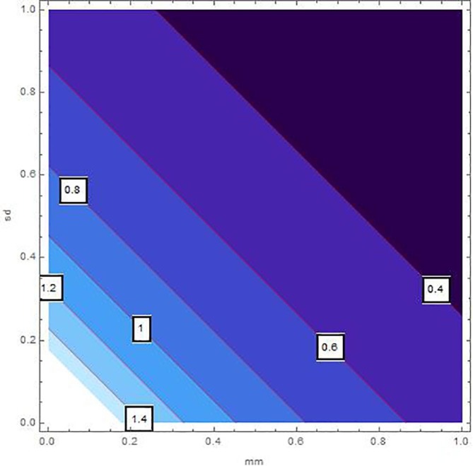
Sensitivity inspection of $R_0$ with respect to $\mathit{mm}$ and $\mathit{sd}$ for $\mathit{ch}=0.1,sc=0.1$, at $\alpha =0.95$.

Fig. 3.

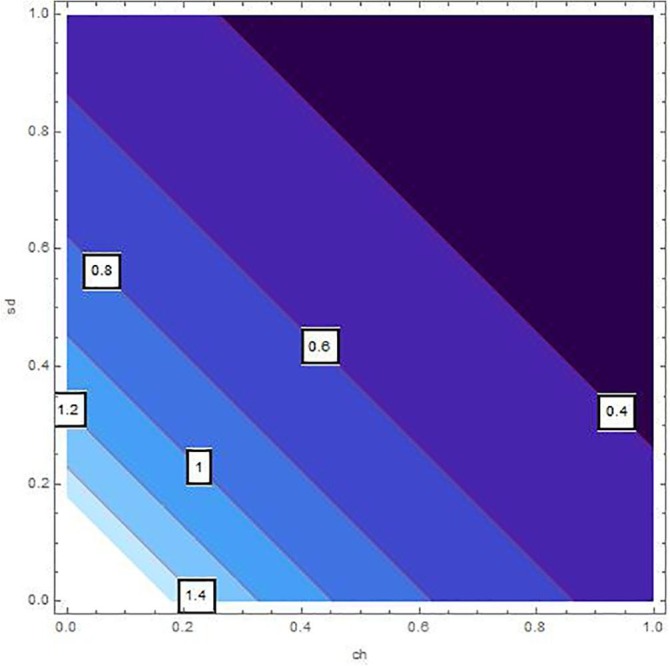
Sensitivity inspection of $R_0$ with respect to $\mathit{ch}$ and $\mathit{sd}$ for $\mathit{mm}=0.1,sc=0.1$, at $\alpha =0.95$.

Fig. 4.

Sensitivity inspection of $R_0$ with respect to $\mathit{ch}$ and $\mathit{sc}$ for $\mathit{mm}=0.1,sd=0.1$, at $\alpha =0.95$.

Fig. 5.

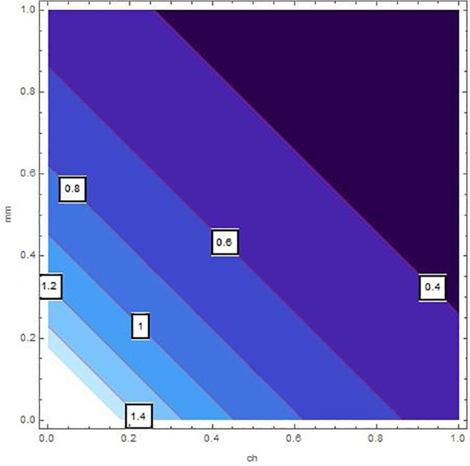
Sensitivity inspection of $R_0$ with respect to $\mathit{ch}$ and $\mathit{mm}$ for $\mathit{sd}=0.1,sc=0.1$, at $\alpha =0.95$.

Fig. 6.

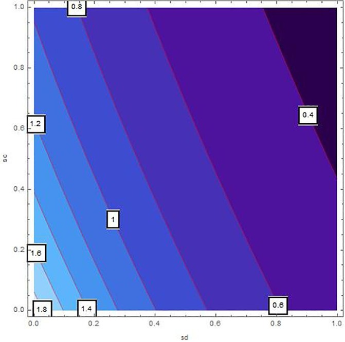
Sensitivity inspection of $R_0$ with respect to $\mathit{sd}$ and $\mathit{sc}$ for $\mathit{mm}=0.1,ch=0.1$, at $\alpha =0.95$.

Fig. 7.

Sensitivity inspection of $R_0$ with respect to $\mathit{mm}$ and $\mathit{sc}$ for $\mathit{sd}=0.1,ch=0.1$, at $\alpha =0.95$.

Equilibrium states and optimality

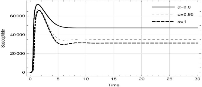
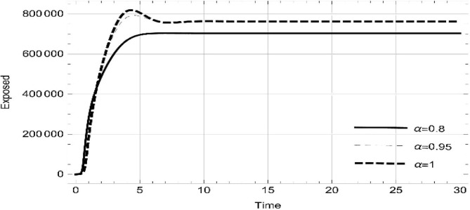
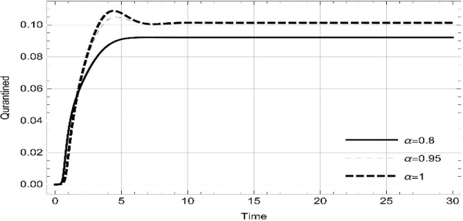
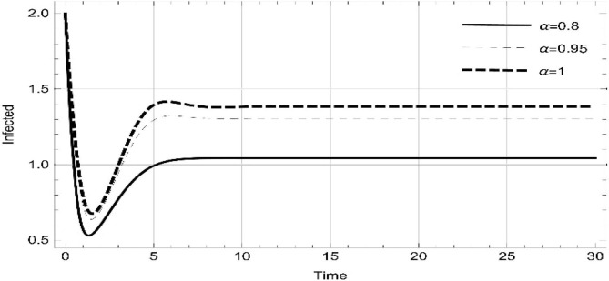
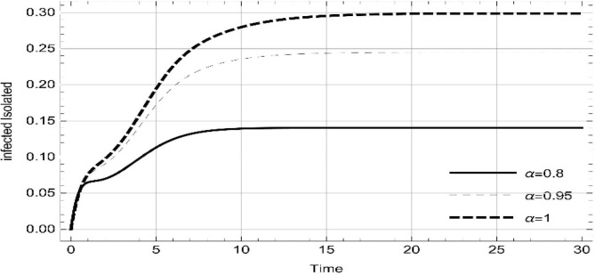
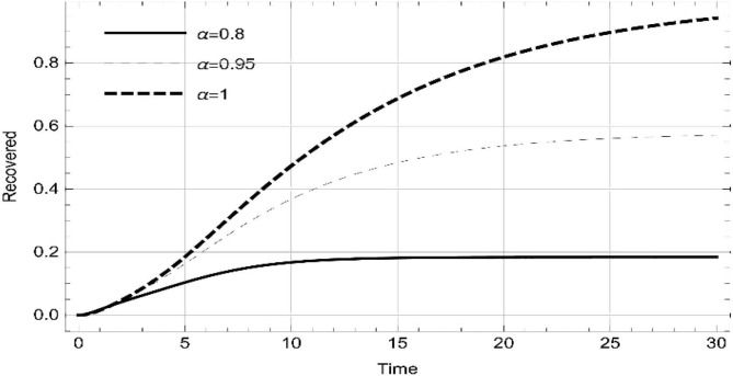
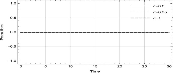
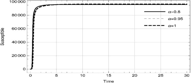
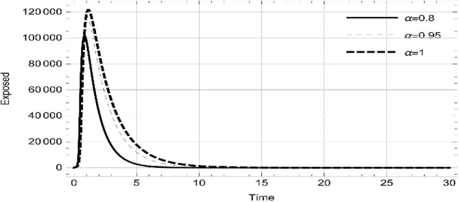
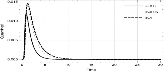
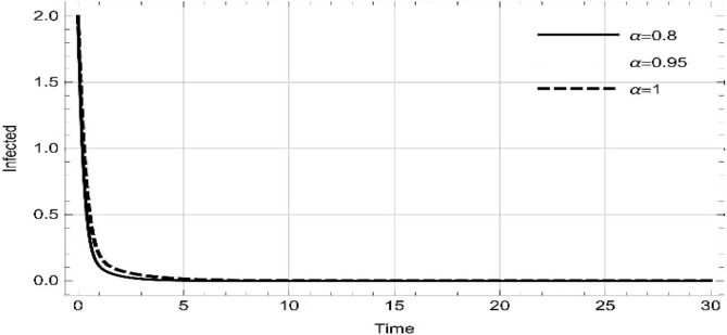
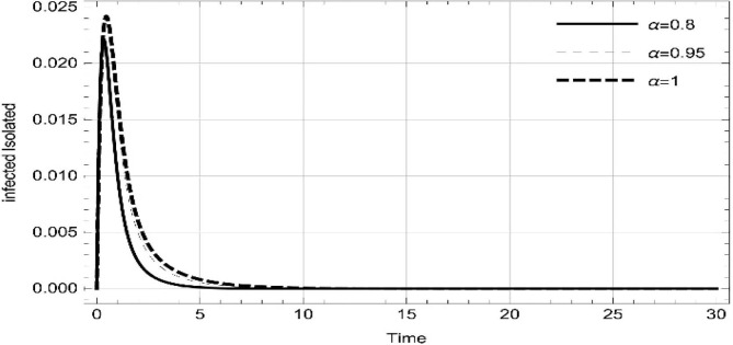
Moreover, solving SEQIMRP system different plots are attained that define the stability of ${\mathrm{\Pi }}_1$ and ${\mathrm{\Pi }}_2$. In the current scenario, evaluations of these equilibrium points are produced on the basis of the prevention campaigns. Commencing from Table 3 , the values are generated for $\mathit{mm}=0,sd=0,ch=0$ and $\mathit{sc}=0$, at $\alpha \in \left(0,1\right]$and $t\in \left[0,30\right]$. Manifestly, it can be seen when no prevention measures are taken $R_0$ increases gradually and endemic state of the pandemic becomes stable. Additionally, Fig. 8, Fig. 9, Fig. 10, Fig. 11, Fig. 12, Fig. 13, Fig. 14 also plotted for $\mathit{mm}=0,sd=0,ch=0$ and $\mathit{sc}=0$, at $\alpha =0.8,0.95,1$ and $t\in \left[0,30\right]$ represent the stability of the deadly endemic state of COIVD'19 for the current rate of transmission, recovery and mortality. Since, no prevention measures are taken at initial spread stage of COVID'19, therefore the curve of protected population yields a constant straight line on zero. This further elaborates the circumstances where everyone is at high risk of being infected that the pandemic situation becomes worst.

Table 3.

Basic reproduction number $R_0$ and endemic equilibrium points ${\mathrm{\Pi }}_2$, for parameters describe in Table 1, for $\mathit{mm}=0,sd=0,ch=0$ and $\mathit{sc}=0$, at different values of $\alpha$and $t\in \left[0,30\right]$.

$\alpha$	$R_0$	$S\left(t\right)$	$E\left(t\right)$	$Q\left(t\right)$	$I\left(t\right)$	$M\left(t\right)$	$R\left(t\right)$	$P\left(t\right)$
0.4	1.07658	90564.3	130,860	0.0166747	0.14077	0.0108021	0.00775503	0
0.5	1.2482	78379.6	341,367	0.0437936	0.394839	0.0339465	0.0267258	0
0.6	1.46208	67141.9	503,966	0.0650954	0.629689	0.0615493	0.0546976	0
0.7	1.73309	56834.8	623,165	0.0810462	0.84565	0.0957691	0.100128	0
0.8	2.08323	47,442	703,299	0.0921023	1.04305	0.140393	0.184117	0
0.9	2.54613	38947.9	748,529	0.0987099	1.22222	0.202724	0.373485	0
1.	3.17529	31335.7	762,847	0.101305	1.38348	0.298912	1.00458	0

Fig. 8.

Dynamics of $S\left(t\right)\in {\mathrm{\Pi }}_2$ of SEQIMRP, for parameters described in Table 1 and $\mathit{mm}=0,sd=0,ch=0$ and $\mathit{sc}=0$, at $\alpha =0.8,0.95,1$and $t\in \left[0,30\right]$.

Fig. 9.

Dynamics of $E\left(t\right)\in {\mathrm{\Pi }}_2$ of SEQIMRP, for parameters described in Table 1 and $\mathit{mm}=0,sd=0,ch=0$ and $\mathit{sc}=0$, at $\alpha =0.8,0.95,1$and $t\in \left[0,30\right]$.

Fig. 10.

Dynamics of $Q\left(t\right)\in {\mathrm{\Pi }}_2$ of SEQIMRP, for parameters described in Table 1 and $\mathit{mm}=0,sd=0,ch=0$ and $\mathit{sc}=0$, at $\alpha =0.8,0.95,1$and $t\in \left[0,30\right]$.

Fig. 11.

Dynamics of $I\left(t\right)\in {\mathrm{\Pi }}_2$ of SEQIMRP, for parameters described in Table 1 for $\mathit{mm}=0,sd=0,ch=0$ and $\mathit{sc}=0$, at $\alpha =0.8,0.95,1$and $t\in \left[0,30\right]$.

Fig. 12.

Dynamics of $M\left(t\right)\in {\mathrm{\Pi }}_2$ of SEQIMRP, for parameters described in Table 1 and $\mathit{mm}=0,sd=0,ch=0$ and $\mathit{sc}=0$, at $\alpha =0.8,0.95,1$and $t\in \left[0,30\right]$.

Fig. 13.

Dynamics of $R\left(t\right)\in {\mathrm{\Pi }}_2$ of SEQIMRP, for parameters described in Table 1 and $\mathit{mm}=0,sd=0,ch=0$ and $\mathit{sc}=0$, at $\alpha =0.8,0.95,1$and $t\in \left[0,30\right]$.

Fig. 14.

Dynamics of $P\left(t\right)\in {\mathrm{\Pi }}_2$ of SEQIMRP, for parameters described in Table 1 and $\mathit{mm}=0,sd=0,ch=0$ and $\mathit{sc}=0$, at $\alpha =0.8,0.95,1$and $t\in \left[0,30\right]$.

Contrarily Table 4 depicts the values, which are generated for $\mathit{mm}=0.2,sd=0.3,ch=0.35$ and $\mathit{sc}=0.65$, at $\alpha \in \left(0,1\right]$ and $t\in \left[0,30\right]$. Evidently from Table 4, when prevention measures are taken into account to some extent, we attain the disease-free state of the dynamics at each value of $\alpha$. In addition, it also shows the value of $R_0$ to be less than one, which is proved in Theorem 4. Fig. 15, Fig. 16, Fig. 17, Fig. 18, Fig. 19, Fig. 20, Fig. 21 graphically demonstrate the stability of ${\mathrm{\Pi }}_1$ for $\mathit{mm}=0.2,sd=0.3,ch=0.35$ and $\mathit{sc}=0.65$, at $\alpha =0.8,0.95,1$ and $t\in \left[0,30\right]$. Contrary to endemic, in disease free case the infected cells become zero whereas susceptible and protected individuals remain at a population level other than zero. Running awareness campaigns about using mask, social distancing, hand wash and also invigorating supportive care of the patients will decrease the basic reproduction number and eventually the deadly spread of COVID'19.

Table 4.

Basic reproduction number $R_0$ and disease free equilibrium points ${\mathrm{\Pi }}_1$, for parameters describe in Table 1, for $\mathit{mm}=0.2,sd=0.3,ch=0.35$ and $\mathit{sc}=0.65$, at different values of $\alpha$and $t\in \left[0,30\right]$.

$\alpha$	$R_0$	$S\left(t\right)$	$E\left(t\right)$	$Q\left(t\right)$	$I\left(t\right)$	$M\left(t\right)$	$R\left(t\right)$	$P\left(t\right)$
0.4	0.297661	94566.7	0	0	0	0	0	97904.3
0.5	0.324551	94,900	0	0	0	0	0	111,349
0.6	0.354992	95233.3	0	0	0	0	0	128,931
0.7	0.389628	95566.7	0	0	0	0	0	152,907
0.8	0.429253	95,900	0	0	0	0	0	187,538
0.9	0.474857	96233.3	0	0	0	0	0	241,958
1.	0.527691	96566.7	0	0	0	0	0	339,915

Fig. 15.

Dynamics of $S\left(t\right)\in {\mathrm{\Pi }}_1$ of SEQIMRP, for parameters described in Table 1 and $\mathit{mm}=0.2,sd=0.3,ch=0.35$ and $\mathit{sc}=0.65$, at $\alpha =0.8,0.95,1$and $t\in \left[0,30\right]$.

Fig. 16.

Dynamics of $E\left(t\right)\in {\mathrm{\Pi }}_1$ of SEQIMRP, for parameters described in Table 1 and $\mathit{mm}=0.2,sd=0.3,ch=0.35$ and $\mathit{sc}=0.65$, at $\alpha =0.8,0.95,1$and $t\in \left[0,30\right]$.

Fig. 17.

Dynamics of $Q\left(t\right)\in {\mathrm{\Pi }}_1$ of SEQIMRP, for parameters described in Table 1 and $\mathit{mm}=0.2,sd=0.3,ch=0.35$ and $\mathit{sc}=0.65$, at $\alpha =0.8,0.95,1$and $t\in \left[0,30\right]$.

Fig. 18.

Dynamics of $I\left(t\right)\in {\mathrm{\Pi }}_1$ of SEQIMRP, for parameters described in Table 1 and $\mathit{mm}=0.2,sd=0.3,ch=0.35$ and $\mathit{sc}=0.65$, at $\alpha =0.8,0.95,1$and $t\in \left[0,30\right]$.

Fig. 19.

Dynamics of $M\left(t\right)\in {\mathrm{\Pi }}_1$ of SEQIMRP, for parameters described in Table 1 and $\mathit{mm}=0.2,sd=0.3,ch=0.35$ and $\mathit{sc}=0.65$, at $\alpha =0.8,0.95,1$and $t\in \left[0,30\right]$.

Fig. 20.

Dynamics of $R\left(t\right)\in {\mathrm{\Pi }}_1$ of SEQIMRP, for parameters described in Table 1 and $\mathit{mm}=0.2,sd=0.3,ch=0.35$ and $\mathit{sc}=0.65$, at $\alpha =0.8,0.95,1$and $t\in \left[0,30\right]$.

Fig. 21.

Dynamics of $P\left(t\right)\in {\mathrm{\Pi }}_1$ of SEQIMRP, for parameters described in Table 1 and $\mathit{mm}=0.2,sd=0.3,ch=0.35$ and $\mathit{sc}=0.65$, at $\alpha =0.8,0.95,1$and $t\in \left[0,30\right]$.

Conclusion

The declaration of PHEIC by the WHO about the COVID'19 outbreak, agitate the scientific community and the healthcare professionals of the countries. After the failure of several experiments on the inoculations, the only operational plan of action to decelerate the spread of COVID'19 is to adopt non-pharmaceutical restrictions. For this purpose, different unprecedented measures are taken into account such as lockdown, closure of institutions and initiating different awareness campaigns. Here, we discussed the cost and public effectiveness of the awareness campaigns taken into consideration by the stakeholders. These maneuvers include the strict imposition of using medical mask in public places, social distancing of 6 feet, frequent use of hand wash and sanitizers, training medical staffs and officers for extraordinary supportive care of COVID'19 patients in hospitals. The optimal control function was designed with the epidemic dynamical system SEQIMRP to mutually study its dynamical stability and the feasibility of the prevention tactics. The system was formulated with the proportional fractional derivative, in order to analyze the basic reproduction number at each chronological change. Ultimately, through the aforementioned analytical and numerical illustrations, the following propitious facts can be extracted:

• •The strategies of using medical mask, social distancing, frequently sanitizing hands and supportive care of COVID'19 for speedy recovery are significant attempts to win this battle against this pandemic.
• •The awareness and necessitating of these lines of attacks may change the state of pandemic into a stable disease-free environment.
• •These can greatly lesser the basic reproduction number from $R_0>1$ to $R_0<1$.
• •The optimal surveillance mitigation with respect to cost effectiveness, social distancing and supportive care may reduce the diffusion of COVID'19 more hastily.
• •Illustrations at different fractional derivative index show systematic reading in the susceptible, expose, quarantined, infected, isolated, recovered and protected population.
• •Without precautions, as the fractional derivative approaches the whole change, the readings represent step by step increase in susceptible, expose, quarantined, infected, isolated and recovered population.
• •Following precautions, as the fractional derivative approaches the whole change, the number individuals in protection increases gradually, while expose, quarantined, infected, isolated and recovered remain zero.
• •Competency in prior recognition of the track of COVID'19 transmission risk through the proportional fractional derivative model.
• •Proficiently trace the basic reproduction number and take preparatory measures before becoming a deadly pandemic.

In the current phase, understanding the epidemiological characteristics is a serious bone of contention question for researchers and health professionals. The successful investigations may significantly help out the stakeholders in making effective standard operational procedures of interventions. The designed model SEQIMRP will categorically aid a great contribution in dynamically scrutinizing and exhibiting the optimal strategy to control the deadly escalation of COVID'19.

Funding

This research received no external funding.

Declaration of Competing Interest

The authors declare that they have no known competing financial interests or personal relationships that could have appeared to influence the work reported in this paper.

References

- 1.Prather K.A., Wang C.C., Schooley R.T. Reducing transmission of SARS-CoV-2. Science. 2020;368(6498):1422–1424. doi: 10.1126/science.abc6197. [DOI] [PubMed] [Google Scholar]
- 2.Van Bavel J.J. Using social and behavioural science to support COVID-19 pandemic response. Nat Hum Behav. 2020:1–12. doi: 10.1038/s41562-020-0884-z. [DOI] [PubMed] [Google Scholar]
- 3.Haushofer J., Metcalf C.J.E. Which interventions work best in a pandemic? Science. 2020;368(6495):1063–1065. doi: 10.1126/science.abb6144. [DOI] [PubMed] [Google Scholar]
- 4.Larson H.J. A call to arms: helping family, friends and communities navigate the COVID-19 infodemic. Nat Rev Immunol. 2020;20(8):449–450. doi: 10.1038/s41577-020-0380-8. [DOI] [PMC free article] [PubMed] [Google Scholar]
- 5.Breevoort A., Carosso G.A., Mostajo-Radji M.A. High-altitude populations need special considerations for COVID-19. Nat Commun. 2020;11(1):1–3. doi: 10.1038/s41467-020-17131-6. [DOI] [PMC free article] [PubMed] [Google Scholar]
- 6.Walker P.G. The impact of COVID-19 and strategies for mitigation and suppression in low-and middle-income countries. Science. 2020 doi: 10.1126/science.abc0035. [DOI] [PMC free article] [PubMed] [Google Scholar]
- 7.Cobey S. Modeling infectious disease dynamics. Science. 2020;368(6492):713–714. doi: 10.1126/science.abb5659. [DOI] [PubMed] [Google Scholar]
- 8.Dobson A.P. Ecology and economics for pandemic prevention. Science. 2020;369(6502):379–381. doi: 10.1126/science.abc3189. [DOI] [PubMed] [Google Scholar]
- 9.Wood H. New insights into the neurological effects of COVID-19. Nature Reviews Neurology. 2020:1. doi: 10.1038/s41582-020-0386-7. [DOI] [PMC free article] [PubMed] [Google Scholar]
- 10.Mangoni, L. and M. Pistilli, Epidemic analysis of Covid-19 in Italy by dynamical modelling. Available at SSRN 3567770, 2020.
- 11.Annas S. Stability analysis and numerical simulation of SEIR model for pandemic COVID-19 spread in Indonesia. Chaos, Solitons Fractals. 2020;139:110072. doi: 10.1016/j.chaos.2020.110072. [DOI] [PMC free article] [PubMed] [Google Scholar]
- 12.Li, J., et al., Estimation of the epidemic properties of the 2019 novel coronavirus: A mathematical modeling study. 2020.
- 13.Nishiga M. COVID-19 and cardiovascular disease: from basic mechanisms to clinical perspectives. Nat Rev Cardiol. 2020;17(9):543–558. doi: 10.1038/s41569-020-0413-9. [DOI] [PMC free article] [PubMed] [Google Scholar]
- 14.Rutz C. COVID-19 lockdown allows researchers to quantify the effects of human activity on wildlife. Nat Ecol Evol. 2020;4(9):1156–1159. doi: 10.1038/s41559-020-1237-z. [DOI] [PubMed] [Google Scholar]
- 15.Habersaat K.B. Ten considerations for effectively managing the COVID-19 transition. Nat Hum Behav. 2020;4(7):677–687. doi: 10.1038/s41562-020-0906-x. [DOI] [PubMed] [Google Scholar]
- 16.Liang W. Early triage of critically ill COVID-19 patients using deep learning. Nat Commun. 2020;11(1) doi: 10.1038/s41467-020-17280-8. [DOI] [PMC free article] [PubMed] [Google Scholar]
- 17.Qureshi S., Yusuf A. Fractional derivatives applied to MSEIR problems: Comparative study with real world data. Eur. Phys. J. Plus. 2019;134(4) doi: 10.1140/epjp/i2019-12661-7. [DOI] [Google Scholar]
- 18.Abbasi Z. Optimal Control Design of Impulsive SQEIAR Epidemic Models with Application to COVID-19. Chaos, Solitons Fractals. 2020;139:110054. doi: 10.1016/j.chaos.2020.110054. [DOI] [PMC free article] [PubMed] [Google Scholar]
- 19.Wang, R. and Q. Wang, Determination and estimation of optimal quarantine duration for infectious diseases with application to data analysis of COVID-arXiv preprint arXiv:2006.05002, 2020. [DOI] [PMC free article] [PubMed]
- 20.Yaro D. Analysis and Optimal Control of Fractional-Order Transmission of a Respiratory Epidemic Model. Int. J. Appl. Comput. Math. 2019;5(4) doi: 10.1007/s40819-019-0699-7. [DOI] [PMC free article] [PubMed] [Google Scholar]
- 21.Yousefpour A., Jahanshahi H., Bekiros S. Optimal policies for control of the novel coronavirus (COVID-19) Chaos, Solitons Fractals. 2020 doi: 10.1016/j.chaos.2020.109883. [DOI] [PMC free article] [PubMed] [Google Scholar]
- 22.Kouidere A. A mathematical modeling with optimal control strategy of transmission of COVID-19 pandemic virus. Commun. Math. Biol. Neurosci. 2020;2020 [Google Scholar]
- 23.Khajji B. A multi-region discrete time mathematical modeling of the dynamics of Covid-19 virus propagation using optimal control. J. Appl. Math. Comput. 2020;64(1-2):255–281. doi: 10.1007/s12190-020-01354-3. [DOI] [PMC free article] [PubMed] [Google Scholar]
- 24.Tajadodi H. Optimal control problems with Atangana-Baleanu fractional derivative. Optimal Control Applications and Methods. 2020 [Google Scholar]
- 25.Grigorieva, E., E. Khailov, and A. Korobeinikov, Optimal quarantine strategies for covid-19 control models. arXiv preprint arXiv:2004.10614, 2020. [DOI] [PMC free article] [PubMed]
- 26.Ullah S., Khan M.A. Modeling the impact of non-pharmaceutical interventions on the dynamics of novel coronavirus with optimal control analysis with a case study. Chaos, Solitons Fractals. 2020;139:110075. doi: 10.1016/j.chaos.2020.110075. [DOI] [PMC free article] [PubMed] [Google Scholar]
- 27.Ahmed I. Analysis of Caputo fractional-order model for COVID-19 with lockdown. Adv Differ Equ. 2020;2020(1) doi: 10.1186/s13662-020-02853-0. [DOI] [PMC free article] [PubMed] [Google Scholar]
- 28.Rahman M.U. Investigating a nonlinear dynamical model of COVID-19 disease under fuzzy caputo, random and ABC fractional order derivative. Chaos, Solitons Fractals. 2020;140 doi: 10.1016/j.chaos.2020.110232. [DOI] [PMC free article] [PubMed] [Google Scholar]
- 29.Jarad F., Abdeljawad T., Alzabut J. Generalized fractional derivatives generated by a class of local proportional derivatives. Eur. Phys. J. Spec. Top. 2017;226(16-18):3457–3471. [Google Scholar]
- 30.Çakan S. Dynamic Analysis of a Mathematical Model with Health Care Capacity for Pandemic COVID-19. Chaos, Solitons Fractals. 2020 doi: 10.1016/j.chaos.2020.110033. [DOI] [PMC free article] [PubMed] [Google Scholar]
- 31.El-Saka H.A.A., Arafa A.A.M., Gouda M.I. Dynamical analysis of a fractional SIRS model on homogenous networks. Advances in Difference Equations. 2019;2019(1):144. [Google Scholar]
- 32.Khan N.A. Fractional order ecological system for complexities of interacting species with harvesting threshold in imprecise environment. Adv Differ Equ. 2019;2019(1) doi: 10.1186/s13662-019-2331-x. [DOI] [Google Scholar]
- 33.Ahmed E., El-Sayed A.M.A., El-Saka H.A.A. On some Routh–Hurwitz conditions for fractional order differential equations and their applications in Lorenz, Rössler, Chua and Chen systems. Phys Lett A. 2006;358(1):1–4. [Google Scholar]
- 34.Razzaq O.A. Economic Growth by Means of Interspecific Functional Response of Capital-Labour in Dynamical System. International Journal of Analysis and Applications. 2019;17(4):630–651. [Google Scholar]
- 35.COVID-19 CORONAVIRUS PANDEMIC. Worldometers.