Constrained spherical deconvolution of nonspherically sampled diffusion MRI data

Abstract

Constrained spherical deconvolution (CSD) of diffusion‐weighted MRI (DW‐MRI) is a popular analysis method that extracts the full white matter (WM) fiber orientation density function (fODF) in the living human brain, noninvasively. It assumes that the DW‐MRI signal on the sphere can be represented as the spherical convolution of a single‐fiber response function (RF) and the fODF, and recovers the fODF through the inverse operation. CSD approaches typically require that the DW‐MRI data is sampled shell‐wise, and estimate the RF in a purely spherical manner using spherical basis functions, such as spherical harmonics (SH), disregarding any radial dependencies. This precludes analysis of data acquired with nonspherical sampling schemes, for example, Cartesian sampling. Additionally, nonspherical sampling can also arise due to technical issues, for example, gradient nonlinearities, resulting in a spatially dependent bias of the apparent tissue densities and connectivity information. Here, we adopt a compact model for the RFs that also describes their radial dependency. We demonstrate that the proposed model can accurately predict the tissue response for a wide range of b‐values. On shell‐wise data, our approach provides fODFs and tissue densities indistinguishable from those estimated using SH. On Cartesian data, fODF estimates and apparent tissue densities are on par with those obtained from shell‐wise data, significantly broadening the range of data sets that can be analyzed using CSD. In addition, gradient nonlinearities can be accounted for using the proposed model, resulting in much more accurate apparent tissue densities and connectivity metrics.

Nonspherically sampled diffusion MRI data can arise either by choice of the sampling scheme (such as diffusion spectrum imaging) or due to gradient nonlinearities, precluding spherical deconvolution (SD) analysis. We adopt a compact response function model that accurately describes the b‐value dependency, enabling SD of nonspherically sampled data and the correction of gradient nonlinearities. With the proposed method, a broader range of data sets can be analyzed with SD approaches, as well as allowing more accurate downstream processing such as fiber tracking and connectomics.

1. INTRODUCTION

Diffusion‐weighted MRI (DW‐MRI) can probe tissue microstructure in a completely noninvasive manner, in vivo. This is achieved by measuring the signal attenuation due to the random motion of water molecules within the tissue of interest (Stejskal & Tanner, 1965). In brain white matter (WM) fibers, the coherent arrangement imparts a directional dependence on the DW signal (Moseley et al., 1990). By measuring this signal along several noncollinear directions, it is possible to estimate the local WM fiber orientations (Dell'Acqua & Tournier, 2019). This information can be used to perform fiber tractography and investigate the long‐range connections between different regions in the brain (Jeurissen, Descoteaux, Mori, & Leemans, 2019).

A widely used approach to estimate the local fiber orientations is spherical deconvolution (SD) (Tournier, Calamante, & Connelly, 2007; Tournier, Calamante, Gadian, & Connelly, 2004), which estimates the fiber orientation density function (fODF) in each voxel, irrespective of the amount of underlying WM fiber populations. SD assumes that the DW signal in a single WM voxel, when sampled in many directions with a constant b‐value (i.e., sampled on a single shell), can be represented as the spherical convolution of the WM response function (RF) and the fODF. The WM RF is the DW signal of a single bundle of coherently oriented WM fibers. If this function is known, it is possible to deconvolve the signal with the RF to infer the fODF.

While SD can provide high‐quality fODF estimates in pure WM, in voxels partially containing other tissue types a single RF is no longer appropriate and produces unreliable, noisy fiber orientation estimates. To address this issue, multitissue SD (MT‐SD) of multishell DW‐MRI data exploits the unique b‐value dependences of the different tissue types to tease them apart (Jeurissen, Tournier, Dhollander, Connelly, & Sijbers, 2014). By sampling the DW signal with multiple b‐values (i.e., multiple shells) and estimating the RFs for each tissue type, it is possible to find the apparent tissue densities as well as the fODFs.

The WM RF is of critical importance for the accurate estimation of the fODF. Ideally, it corresponds to the DW signal that would be acquired for a unit volume of WM coherently aligned along a single axis. It can be obtained directly from the data by selecting voxels that are deemed to contain a single coherent fiber bundle (Tournier et al., 2004, 2007) either by explicit thresholding of brain regions with high fractional anisotropy (FA) (Tournier et al., 2004), or through recursive calibration of the fiber response (Tournier, Calamante, & Connelly, 2013). Because the signal response for each b‐value is a function over the sphere, spherical harmonics (SH) basis functions are a natural candidate for a parametric representation. However, a limitation of using SH coefficients is that their estimation requires the DW measurements to be densely distributed on shells in b‐space. Due to this, data acquired with sparse shell samplings cannot be readily analyzed with SD. In addition, nonspherical sampling schemes such as Cartesian sampling used in diffusion spectrum imaging (DSI) (Wedeen, Hagmann, Tseng, Reese, & Weisskoff, 2005) or CUbe and SPhere acquisitions (Scherrer & Warfield, 2012) preclude SD‐analysis as well.

Moreover, the physical laws that govern magnetic fields can lead to nonspherical DW sampling. Indeed, the Maxwell equations that describe the DW gradients imply transverse magnetic field components that contribute to undesirable spatial dependencies of the b‐values and DW directions across the brain (Bammer et al., 2003; Baron, Lebel, Wilman, & Beaulieu, 2012; Borkowski & KrzyŻak, 2018; Mesri, David, Viergever, & Leemans, 2019). As the magnitude of these concomitant fields increases with the square of the gradient strength, high quality data sets acquired with strong gradients, like those of the Human Connectome Project (HCP), are subjected to significant nonlinearities (Sotiropoulos et al., 2013). However, the SH representation of the RFs assumes perfect spherical sampling with spatially invariant b‐values, an assumption that is invalidated as a result of these nonlinearities.

Second‐order tensor models have also been used to represent RFs and are compatible with nonspherically sampled DW data sets (Anderson, 2005; Dell'Acqua et al., 2007; Kaden, Knösche, & Anwander, 2007). However, their inability to accurately represent the nonmonoexponential decay of the DW signal at higher b‐values limits their applicability in modern DW data sets (Jensen & Helpern, 2010). The Simple Harmonic Oscillator‐based Reconstruction and Estimation (SHORE) basis is capable of describing both the angular and radial dependencies of the DW signal (Özarslan, Koay, & Basser, 2013), but requires a larger number of parameters to achieve this.

In this work, we employ a compact higher‐order tensor model that provides an accurate description of the tissue RFs over a continuous range of b‐values and directions, and we apply it to SD of nonspherically sampled DW data sets.

Note that Guo, Leemans, Viergever, Dell'Acqua, and de Luca (2020) simultaneously proposed a multishell SD approach that could, in principle, also be used to perform SD of nonspherically sampled DW data.

2. THEORY

2.1. Spherical deconvolution

SD assumes that the DW signal results from the spherical convolution of the RF and the fODF:

$$S_b\left(\mathit{g}\right)={\int }_{S^2}{R}_b\left(\mathit{g};\mathit{n}\right)f\left(\mathit{n}\right)d\mathit{n}=R_b\otimes f$$ (1)

with S _b(g) the measured DW signal for some magnetic field gradient direction g (with |g| = 1) and at a constant b‐value. The signal response at a constant b‐value of a single fiber population along a direction n for a gradient direction g is denoted with R _b(g;n). The quantity of interest, the fODF f(n), represents the density of fibers in the direction n. If R _b(g;n) is known, the fODF can be obtained from the measured signal S _b(g) using SD:

$$\widehat{f}\left(\mathit{n}\right)=R_b\left(\mathit{g};\mathit{n}\right){\otimes }^{-1}{S}_b\left(\mathit{g}\right)$$ (2)

Since deconvolution is ill‐conditioned, a nonnegativity constraint is typically imposed to prevent unphysical negative amplitudes in the estimated fODF, a technique referred to as constrained SD (Tournier et al., 2007).

2.2. RF parametrization

2.2.1. Per b‐value parametrization

Currently, RFs are parametrized per b‐value using real‐valued SH coefficients (truncated up to a maximum harmonic order l = l _max):

$$R_b\left(\mathit{g}\right)=\sum _{l=0}^{l_{\mathit{max}}}\sum _{m=-l}^l{c}_l^m{Y}_l^m\left(\mathit{g}\right)$$ (3)

where R _b(g) is the signal response at a constant b‐value for a single fiber population along the z‐axis, $Y_l^m$ are the SH basis functions, and $c_l^m$ are the series coefficients (Tournier et al., 2007). As R _b(g) exhibits antipodal symmetry in q‐space, only even orders need to be considered. In addition, as WM tissue RFs can be assumed to exhibit axial symmetry about the z‐axis, only the m = 0 SH, also known as the zonal SH (ZSH), have to be taken into account:

$$R_b\left(\mathit{g}\right)=\sum _{l=0,2,\cdots }^{l_{\mathit{max}}}{c}_l^0{Y}_l^0\left(\mathit{g}\right)$$ (4)

Typically, the series is truncated at l _max = 8 for anisotropic tissue types such as WM, resulting in five coefficients to describe the single‐shell response (Tournier et al., 2013). While the ZSH representation is compact, it can only describe the angular dependency of the DW signal. This precludes RF representation of data with nonspherical acquisition schemes. It also means that, in the case of multishell data, the ZSH coefficients are estimated separately for each shell (Jeurissen et al., 2014).

2.2.2. Across b‐value parametrization

Some authors have modeled tissue RFs for variable b‐values using a second‐order tensor model, also known as the diffusion tensor imaging (DTI) model (Anderson, 2005; Dell'Acqua et al., 2007; Kaden et al., 2007):

$$R\left(b,\mathit{g}\right)=S_0{e}^{-\mathit{bD}\left(\mathit{g}\right)}$$ (5)

with S ₀ the signal with no diffusion‐weighting and D(g) the apparent diffusivity in a particular gradient direction g:

$$D\left(\mathit{g}\right)=\sum _{i,j=1}^3{g}_i{D}_{\mathit{ij}}{g}_j$$ (6)

When constraining the DW signal to be axially symmetric (AS) about a known axis, the DTI model simplifies to just three parameters: S ₀, axial diffusivity and radial diffusivity. In this work, this model will be called the DTI AS model. For isotropic RFs, the DTI model requires just two parameters: S ₀ and mean diffusivity (MD). This isotropic model will be referred to as DTI ISO. In principle, such responses enable SD of multishell, as well as nonspherically sampled data. However, the DTI model is known to be a poor fit for data with high b‐values. To address this issue, the model can be extended with a fourth‐order tensor, also known as the diffusion kurtosis imaging (DKI) model (Jensen & Helpern, 2010):

$$R\left(b,\mathit{g}\right)=S_0{e}^{-\mathit{bD}\left(\mathit{g}\right)+b^{2}W\left(\mathit{g}\right)}$$ (7)

with

$$W\left(\mathit{g}\right)=\sum _{i,j,k,l=1}^3{g}_i{g}_j{W}_{\mathit{\text{ijkl}}}{g}_k{g}_l$$ (8)

As opposed to the full DKI model, we assume axial symmetry about a known axis, requiring only six parameters to represent an anisotropic RF across shells (referred to as DKI AS), and three parameters for isotropic RFs (referred to as DKI ISO). A derivation of AS and isotropic fourth‐order tensors is given in the appendix. Note that this simplification is similar in spirit to the model proposed by Hansen, Shemesh, and Jespersen (2016), where axial symmetry was used to reduce minimal acquisition requirements for DKI.

To account for a nondecaying signal component not modeled by DKI, an additional offset parameter C is added to the RF model (Alexander et al., 2010):

$$R\left(b,\mathit{g}\right)=S_0{e}^{-\mathit{bD}\left(\mathit{g}\right)+b^{2}W\left(\mathit{g}\right)}+C$$ (9)

resulting in a total of seven parameters to represent an anisotropic RF across shells (DKI AS + offset), and four parameters in the case of isotropic RFs (DKI ISO + offset).

To ensure that the signal can only decrease with increasing b‐value in any gradient direction we enforce that, for all b ∈ [0, b _max]:

$$\frac{\mathit{dS}}{\mathit{db}}\le 0$$ (10)

as in Tabesh, Jensen, Ardekani, and Helpern (2011). Combining Equations (9) and (10) results in the following linear constraint:

$$2W\left(\mathit{g}\right)b_{\mathit{max}}-D\left(\mathit{g}\right)\le 0$$ (11)

The total amount of parameters n _θ for each response model, as well as their symmetry constraints are listed in Table 1.

TABLE 1.

Breakdown of the number of parameters of the models used to represent the different tissue compartments. The full models without symmetry constraints (DTI and DKI) are included for comparison, but were not used in any experiments. The acronyms “AS” and “ISO” refer to axial symmetry about the z‐axis and isotropic symmetry, respectively. The amount of parameters contributed by each term γ in Equation (9) is denoted with n _γ. The total amount of parameters is denoted with n _γ

Model type	Symmetry	$n_{S_0}$	n D	n W	n C	n γ
DTI	Point	1	6	0	0	7
DKI	Point	1	6	15	0	22
DTI AS	Point + axial	1	2	0	0	3
DKI AS	Point + axial	1	2	3	0	6
DKI AS + offset	Point + axial	1	2	3	1	7
DTI ISO	Isotropic diffusion	1	1	0	0	2
DKI ISO	Isotropic diffusion	1	1	1	0	3
DKI ISO + offset	Isotropic diffusion	1	1	1	1	4

Abbreviations: AS, axially symmetric; DKI, diffusion kurtosis imaging.

2.3. Implementation of the deconvolution operation

The single‐shell constrained SD operation can be formulated as a constrained linear least squares problem of the form:

$$\widehat{\mathit{x}}=\arg \underset{\mathit{x}}{\min }{\left|\left|\mathit{Ax}-\mathit{y}\right|\right|}_2^2\text{subject to}\mathit{Cx}\ge \mathbf{0}$$ (12)

where x is the unknown column vector of coefficients of the fODF, y is the column vector of DW signal intensities measured on a single shell in q‐space, A is the matrix relating the fODF coefficients to the measured DW signal by means of spherical convolution, and C is the matrix relating the fODF coefficients to the fODF amplitudes, effectively enforcing nonnegativity of the fODF.

The convolution matrix A can be decomposed as:

$$\mathit{A}=\mathit{Q}\mathit{R}$$ (13)

where Q is the matrix relating the coefficients of the single‐shell signal to the signal amplitudes, and R is the single‐shell forward convolution matrix in coefficient space. When using the SH basis to represent the functions on the sphere, Q contains the SH basis functions evaluated along the gradient directions, and R can be constructed directly from the ZSH coefficients of the single‐shell response. For a detailed explanation on how to construct R from the ZSH coefficients, see appendix 2 of Tournier et al. (2007).

Jeurissen et al. (2014) showed that Equation (12) can be adapted to accommodate m shells in q‐space:

$$\widehat{\mathit{x}}=\arg \underset{\mathit{x}}{\min }{\left|\left|\left[\begin{array}{l}{\mathit{A}}_1\\ ⋮\\ {\mathit{A}}_m\end{array}\right]\mathit{x}-\left[\begin{array}{l}{\mathit{y}}_1\\ ⋮\\ {\mathit{y}}_m\end{array}\right]\right|\right|}_2^2\text{subject to}\mathit{Cx}\ge \mathbf{0}$$ (14)

where y _i is the column vector of q‐space samples on the ith shell and A _i a matrix relating the fODF coefficients to the DW signal intensities measured on the ith shell through spherical convolution. As in Equation (13), the convolution matrices A _i can be decomposed as:

$${\mathit{A}}_i={\mathit{Q}}_i{\mathit{R}}_i$$ (15)

where Q _i is the matrix relating the coefficients of the signal at the ith shell to the corresponding amplitudes, and R _i is the forward convolution matrix in coefficient space for the ith shell. When using the SH basis to represent the functions on the sphere, Q _i contains the SH basis functions evaluated along the gradient directions of the ith shell and R _i can be constructed directly from the ZSH coefficients of the response as explained above.

In this work, Equation (14) is generalized to accommodate m arbitrary q‐space samples:

$$\widehat{\mathit{x}}=\arg \underset{\mathit{x}}{\min }{\left|\left|\left[\begin{array}{l}{\mathit{a}}_1\\ ⋮\\ {\mathit{a}}_m\end{array}\right]\mathit{x}-\left[\begin{array}{l}{y}_1\\ ⋮\\ y_m\end{array}\right]\right|\right|}_2^2\text{subject to}\mathit{Cx}\ge \mathbf{0}$$ (16)

where y _i are the individual q‐space samples and a _i a vector relating the fODF coefficients to the ith q‐space sample through spherical convolution. The convolution vector a _i can be decomposed as in Equations (13) and (15):

$${\mathit{a}}_i={\mathit{q}}_i{\mathit{R}}_i$$ (17)

where q _i is a vector relating the coefficients of the signal at the b‐value of the ith q‐space sample to the amplitude of the ith q‐space sample, and R _i is the forward convolution matrix in coefficient space for the b‐value of ith q‐space sample. When using the SH basis to represent the functions on the sphere, q _i contains the SH basis functions evaluated along the gradient direction of the ith q‐space sample and R _i can be constructed from the ZSH coefficients of the signal response for the b‐value corresponding to the ith q‐space sample as explained earlier. Because the response model in Equation (9) does not provide ZSH coefficients directly, we instead obtain ZSH coefficients for each q‐space sample by evaluating Equation (9) at the b‐value corresponding to the ith q‐space sample and fitting a ZSH series. Note that this conversion to ZSH is of low computational complexity, as the combined axial and point symmetry of the RF requires evaluation of Equation (9) only on a quarter‐circle (e.g., see Figure 4). Note the data in vector y of Equations (14) and (16), the equations are left untouched and that the SD operation is performed directly on y without any interpolation.

As Equations (12), (14), and (16) are all convex linear least squares problems, they can be solved efficiently using quadratic programming.

3. METHODS

3.1. Data acquisition and preprocessing

Written informed consent was obtained from a healthy adult volunteer according to institutional guidelines. DW‐MRI data were acquired in a single session with both a multishell sampling scheme (DW data set 1a) and a Cartesian sampling scheme (DW data set 1b). The single‐session acquisition facilitates the alignment of all DW volumes across both data sets to allow a straightforward comparison of both sampling strategies. A graphical representation of the q‐space points of both sampling schemes can be appreciated in Figure 1, with $\mid \mathit{q}\mid \propto \sqrt{b}$. The data were acquired on a 3 T Siemens Magnetom Prisma system equipped with a 32‐channel receiver head coil using a pulsed gradient spin echo sequence, with a repetition time TR of 4,500 ms and an echo time TE of 74 ms. Additional acquisition parameters were: voxel size = 2.5 × 2.5 × 2.5 mm³, matrix = 88 × 88, slices = 58, parallel imaging acceleration factor = 2 (GRAPPA), band width = 2,470 Hz/Px. For EPI distortion correction, an additional b = 0 s/mm² image was acquired with reversed phase encoding.

• Data set 1a (spherical sampling): q‐space was sampled at seven shells with b‐values 0; 250; 500; 1,000; 2,000; 3,000; and 4,000 s/mm² containing 11, 45, 45, 45, 45, 66, and 66 directions, respectively, uniformly distributed using electrostatic repulsion (Jones, Horsfield, & Simmons, 1999).

• Data set 1b (Cartesian sampling): q‐space was sampled at an equally spaced Cartesian grid, truncated at b = 4,000 s/mm²), resulting in a total of 267 directions (including 10 volumes with b = 0 s/mm²)

FIGURE 1.

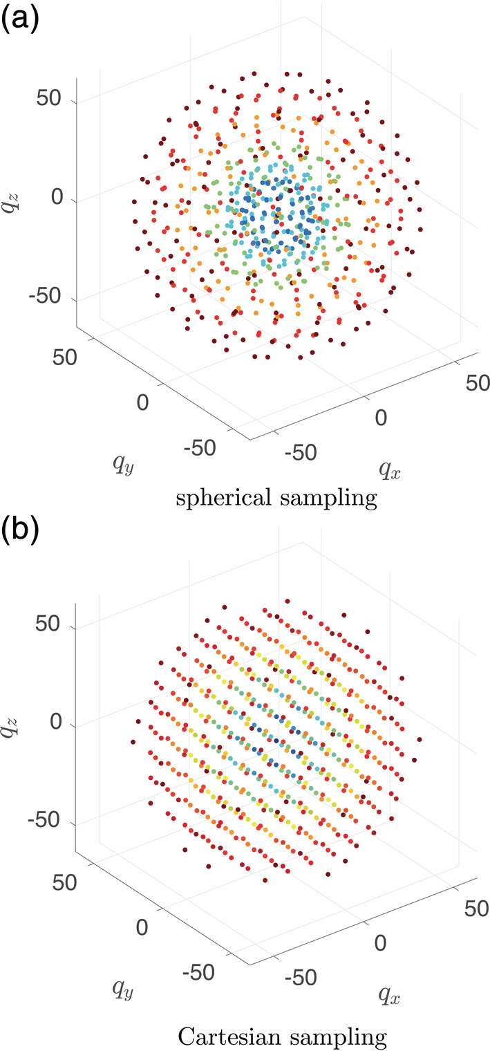
Graphical representation of the diffusion‐weighted (DW) sampling points in q‐space for data set 1: spherical (a) and Cartesian sampling (b). The points are color coded according to the magnitude of the q‐vector

The combined data set (i.e., data sets 1a + 1b) was preprocessed using a state‐of‐the‐art pipeline (Tournier et al., 2019) consisting of: denoising (Veraart et al., 2016), Gibbs‐ringing correction (Kellner, Dhital, and Reisert, 2016), model‐based affine motion and distortion correction (Bai & Alexander, 2008), and bias field correction (Tustison et al., 2010). After preprocessing, the combined data set was split up again in data sets 1a and 1b.

To investigate the effect of the gradient nonlinearities on the fODF parameters, a data set from the HCP was used. This data set is supplied with a map that describes the spatial dependencies of the diffusion sampling scheme as a result of these nonlinearities.

• Data set 2 (spherical sampling): A preprocessed data set from the HCP was used (Glasser et al., 2013) with four shells with b‐values 5; 1,000; 2,000; and 3,000 s/mm² and 18, 90, 90, and 90 directions, respectively. In addition to the standard HCP preprocessing pipeline, bias field correction was performed (Tustison et al., 2010).

To verify the generalizability of our method to even higher b‐values, we used an HCP MGH data set:

• Data set 3 (spherical sampling): A preprocessed HCP MGH data set was used (Glasser et al., 2013) with five shells with b‐values 0; 1,000; 3,000; 5,000; and 10,000 s/mm² and 40, 64, 64, 128, and 256 directions, respectively.

3.2. Estimating tissue RFs

To estimate the RFs from the data, voxels that were deemed to contain just one of the three tissue types (WM, GM, or cerebrospinal fluid [CSF]) were selected by thresholding FA and MD:

• WM: FA > 0.8 and MD < 0.6 μm²/ms.

• GM: FA < 0.1 and MD < 0.6 μm²/ms.

• CSF: FA < 0.1 and MD > 3 μm²/ms.

These DTI metrics were obtained using a weighted linear least squares estimator (Veraart, Sijbers, Sunaert, Leemans, & Jeurissen, 2013). They were estimated from DW data that includes high b‐values, which is known to result in biased DTI metrics Veraart et al. (2011). Note however, that these metrics were used solely to select representative voxels for each tissue type. The DW signals for all single‐tissue voxels were then concatenated into a vector y of length n. In the case of anisotropic tissue types (such as WM), prior to fitting, the gradient directions for each voxel were rotated such that the principal eigenvector coincided with the z‐axis (Tournier et al., 2004). For each of the above models, the response parameter vector θ was estimated, resulting in a single tissue RF for the whole brain:

$$\widehat{\mathit{\theta }}=\arg \underset{\mathit{\theta }}{\min }{\left|\mathit{y}-\mathit{R}\left(b,\mathit{g},\mathit{\theta }\right)\right|}_2^2$$ (18)

where R(b, g, θ) is the signal predicted by one of the candidate models for a given b‐value. Note that in principle, recursive calibration could also be used to estimate the RF (Christiaens, Sunaert, Suetens, & Maes, 2017; Tax, Jeurissen, Vos, Viergever, & Leemans, 2014; Tournier et al., 2013).

3.3. Spherically sampled data experiments

MT responses were modeled with the various models described in Section 2.2 and compared to the state‐of‐the‐art ZSH (with l _max = 8) using the spherically sampled data set 1a. Comparison of the signal responses obtained with each of these models was performed in both the angular (for WM) and the radial domain for WM, GM, and CSF. In addition, the apparent densities of WM, GM, and CSF obtained with said models were compared to those obtained with the state‐of‐the‐art ZSH responses.

To compare the models quantitatively, the root mean squared residual (RMSR) as well as the Akaike Information Criterion (AIC) (Burnham & Anderson, 1998) were employed. The former only takes into account the goodness of fit:

$$\text{RMSR}=\sqrt{\frac{1}{n}\sum _{i=1}^n{\widehat{\mathrm{\epsilon }}}_i^2}$$ (19)

with the residual ${\widehat{\mathrm{\epsilon }}}_i$ defined as the difference between the measured signal y _i and $R\left(b_i,{\mathit{g}}_i,\widehat{\mathit{\theta }}\right)$, the signal predicted by the candidate model:

$${\widehat{\mathrm{\epsilon }}}_i=y_i-R\left(b_i,{\mathit{g}}_i,\widehat{\mathit{\theta }}\right)$$ (20)

The latter also includes a penalty depending on the total amount of response parameters n _θ:

$$\mathrm{AIC}=n\log \left(\frac{1}{n}\sum _{i=1}^n{\widehat{\mathrm{\epsilon }}}_i^2\right)+2n_{\theta }$$ (21)

The stability of the AIC was assessed for each tissue type using the classical bootstrap as in Ferizi et al. (2014). For each bootstrap sample (out of a total of 100), a set of DW samples was selected with replacement in each shell and the RFs were then estimated. Next, the AIC values were calculated for each model and ranked in ascending order, where the lowest AIC value (i.e., the highest ranking) corresponded to the model that best described the data while avoiding overfitting.

3.4. Generalizability to higher b‐values

The generalizability of our method to higher b‐values was tested by fitting the DKI + offset and ZSH models to an ensemble of single‐tissue voxels from data set 3 and comparing the signal responses in the radial domain up to b = 10,000 s/mm².

3.5. Nonspherically sampled data experiments

3.5.1. Cartesian sampling

The RF model parameters of DKI AS + offset (for WM) and DKI ISO + offset (for GM and CSF) were estimated from the spherically sampled data (data set 1a) and the Cartesian sampled data (data set 1b), to ensure that the estimated RFs did not depend on the sampling strategy. Finally, the apparent tissue densities were estimated from data set 1b and compared to those obtained from data set 1a.

3.5.2. Spherical sampling with gradient nonlinearities

The HCP data sets are supplied with a gradient nonlinearity map that enables the calculation of the true DW gradients based on the assumed gradients. Figure 2 a shows the relative deviation (in %) from the nominal b‐values of this gradient nonlinearity map. In practice, this map consists of a spatially dependent linear transform L(r) which maps each gradient vector g of the assumed DW sampling scheme to its true direction and magnitude g′(r) (Bammer et al., 2003):

$$\left[\begin{array}{l}{g}_x^{\prime }\left(\mathit{r}\right)\\ g_y^{\prime }\left(\mathit{r}\right)\\ g_z^{\prime }\left(\mathit{r}\right)\end{array}\right]=\left(\begin{array}{lll}{L}_{\mathit{xx}}\left(\mathit{r}\right)& L_{\mathit{xy}}\left(\mathit{r}\right)& L_{\mathit{xz}}\left(\mathit{r}\right)\\ L_{\mathit{yx}}\left(\mathit{r}\right)& L_{\mathit{yy}}\left(\mathit{r}\right)& L_{\mathit{zy}}\left(\mathit{r}\right)\\ L_{\mathit{zx}}\left(\mathit{r}\right)& L_{\mathit{zy}}\left(\mathit{r}\right)& L_{\mathit{zz}}\left(\mathit{r}\right)\end{array}\right)\left[\begin{array}{l}{g}_x\\ g_y\\ g_z\end{array}\right]$$ (22)

FIGURE 2.

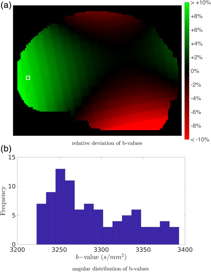
Deviations of the b‐value due to gradient nonlinearities in data set 2: (a) deviation as a function of position (averaged across directions), and (b) distribution of b‐values in a b = 3,000 s/mm² shell (within a single voxel, delineated by the white square in (a))

Because the diffusion weighting scheme is spatially dependent, the MT‐SD convolution matrix has to be adjusted for each voxel. In addition, the linear transform L(r) also imposes an angular dependency on the b‐values. Figure 2b depicts the distribution of the true b‐values in a b = 3,000 s/mm² shell of a HCP data set.

MT‐CSD was performed using the DKI + offset model both with and without taking into account the gradient nonlinearities. The fODFs as well as the apparent densities of WM, GM, and CSF obtained with both approaches were compared to assess the detrimental effects of not accounting for gradient nonlinearities. To assess the impact of gradient nonlinearities on fiber tracking, we also compared connectivity information obtained with both approaches. First, 10 million tracks were generated using probabilistic whole brain fiber tracking using second‐order integration (Tournier, Calamante, & Connelly, 2010). Next, tracks were subjected to SIFT2 to improve the quantitative nature of the whole‐brain tractogram (Smith, Tournier, Calamante, & Connelly, 2015). Finally, a whole brain connectivity matrix was obtained using the Desikan–Killiany parcellation and excluding self‐connections (Desikan et al., 2006). For each brain parcel, we obtained the total connectivity to all other parcels by summing the rows of the connectivity matrix and compared these numbers between both approaches.

4. RESULTS

4.1. Spherically sampled data experiments

Using the spherically sampled data set 1a, the signal predicted by the various response models was compared to that predicted by the state‐of‐the‐art ZSH. Figure 3 shows the tissue response (averaged over the unit sphere) predicted by the different models as a function of b‐value.

FIGURE 3.

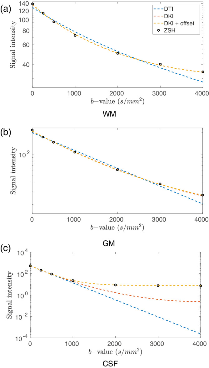
Comparison of the radial component of tissue responses predicted by the candidate models and the zonal spherical harmonics (ZSH) model for (a) white matter (WM), (b) gray matter (GM), and (c) cerebrospinal fluid (CSF) using data set 1a. Note that in Figure 3a the red and yellow dotted lines overlap

For WM, the DTI AS model fails to accurately predict the signal over the entire range of b‐values: for low b‐values (0–250 s/mm²) it underestimates the signal, for intermediate b‐values (500–2,500 s/mm²) it overestimates the signal, and for high b‐values (>2,500 s/mm²) the signal is underestimated (Figure 3a). In contrast, the DKI AS model can predict the signal response accurately over the entire range of b‐values. The signal response predicted by the DKI AS + offset model is equivalent to that predicted by the DKI AS model. The same trends can be observed in GM when using the isotropic models (Figure 3b).

In CSF, the DTI ISO model is able to describe the signal for b‐values up to 500 s/mm². For higher b‐values, the signal is underestimated considerably. The DKI ISO model is able to describe the signal for b‐values up to 1,000 s/mm², but for higher b‐values, considerable underestimation of the signal remains. Finally, the offset parameter of the DKI ISO NF model allows the accurate prediction of the CSF response over the entire range of b‐values, with the prediction closely matching that of the ZSH model (Figure 3c).

In Figure 4, the angular WM responses predicted by the various response models were compared to the ZSH responses. Depending on the b‐value and orientation, the DTI AS model substantially overestimate and underestimate the signal, whereas the DKI AS and DKI AS + offset responses resemble the ZSH response much more closely.

FIGURE 4.

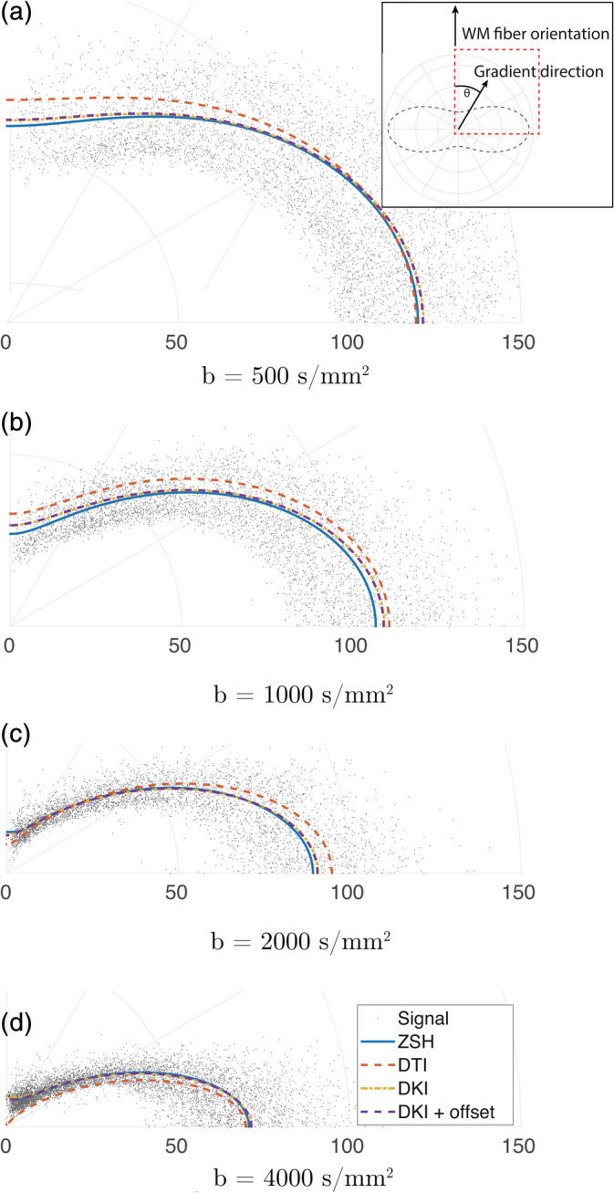
Comparison of the angular component of the white matter (WM) response predicted by the candidate models and the zonal spherical harmonics (ZSH) model using spherically sampled data, at different b‐values. The polar angle θ corresponds with the angle between the b‐vector and the z‐axis. The data points are the measured signals for the ensemble of WM voxels with their principal eigenvector aligned with the z − axis (or equivalently the θ = 0 axis)

A quantitative comparison of the various models with the ZSH can be appreciated in Table 2, which contains the RMSR, as well as the AIC values of the model fits. For all three tissues, moving from DTI to DKI improves both the RMSR and the AIC considerably, as could already be appreciated qualitatively from Figures 3 and 4. The addition of the offset parameter also improves these metrics, but this improvement was only substantial for CSF. This is further confirmed by the results of the AIC bootstrap experiment, which are shown in Figure 5. For all three tissue types, the DTI model consistently has the lowest AIC ranking, and is outranked by the DKI models. For WM and GM, the addition of the offset parameter improves the AIC ranking in the majority but not all of the bootstrap samples, indicating that both higher order models are closely tied. In CSF, on the other hand, the DKI ISO + offset model is the most appropriate, as it is consistently ranked first.

TABLE 2.

Response function model comparison in terms of RMSR and AIC for WM, GM, and CSF, performed on data set 1a. The total amount of parameters n _θ is included in the parentheses after each model name

WM model type (n θ)	RMSR	AIC
DTI AS (3)	12.423	3.02744 × 105
DKI AS (6)	11.370	2.92103 × 105
DKI AS NF (7)	11.369	2.92098 × 105

GM model type (n θ)	RMSR	AIC
DTI ISO (2)	34.077	4.30829 × 105
DKI ISO (3)	33.717	4.29532 × 105
DKI ISO + offset (4)	33.705	4.29491 × 105

CSF model type (n θ)	RMSR	AIC
DTI ISO (2)	30.551	3.62269 × 105
DKI ISO (3)	30.184	3.60991 × 105
DKI ISO + offset (4)	29.630	3.59029 × 105

Abbreviations: AIC, Akaike Information Criterion; AS, axially symmetric; CSF, cerebrospinal fluid; DKI, diffusion kurtosis imaging; GM, gray matter; RMSR, root mean squared residual; WM, white matter.

FIGURE 5.

Response function model Akaike Information Criterion (AIC) ranking distributions obtained from the bootstrapping experiment. The rows correspond to the model type and the columns are the ranking of AIC scores in each bootstrap sample

Figure 6 shows the MT‐SD apparent tissue density maps and a close‐up of the fODFs estimated using the various response models. The shape and orientations of the fODFs are largely unaffected by the choice of response model. To aid comparison of the tissue density maps, Figure 7 shows the relative differences in tissue density (in %), compared to the ZSH model. Figure 8 depicts the distributions of the relative difference maps of Figure 7.

FIGURE 6.

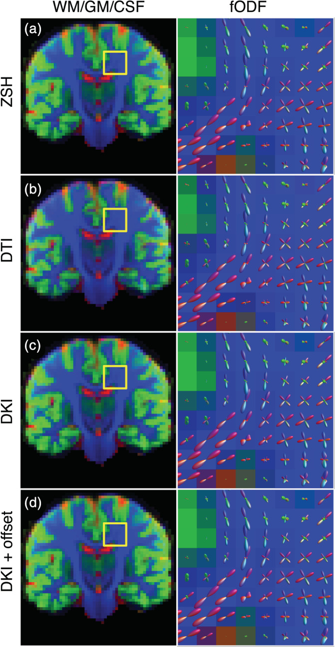
Comparison of the apparent densities (left) and the fiber orientation density functions (fODFs) (right) obtained with the candidate response models and the zonal spherical harmonics (ZSH) model on data set 1a. The apparent densities are shown as RGB maps: cerebrospinal fluid (CSF) (red), gray matter (GM) (green), and white matter (WM) (blue)

FIGURE 7.

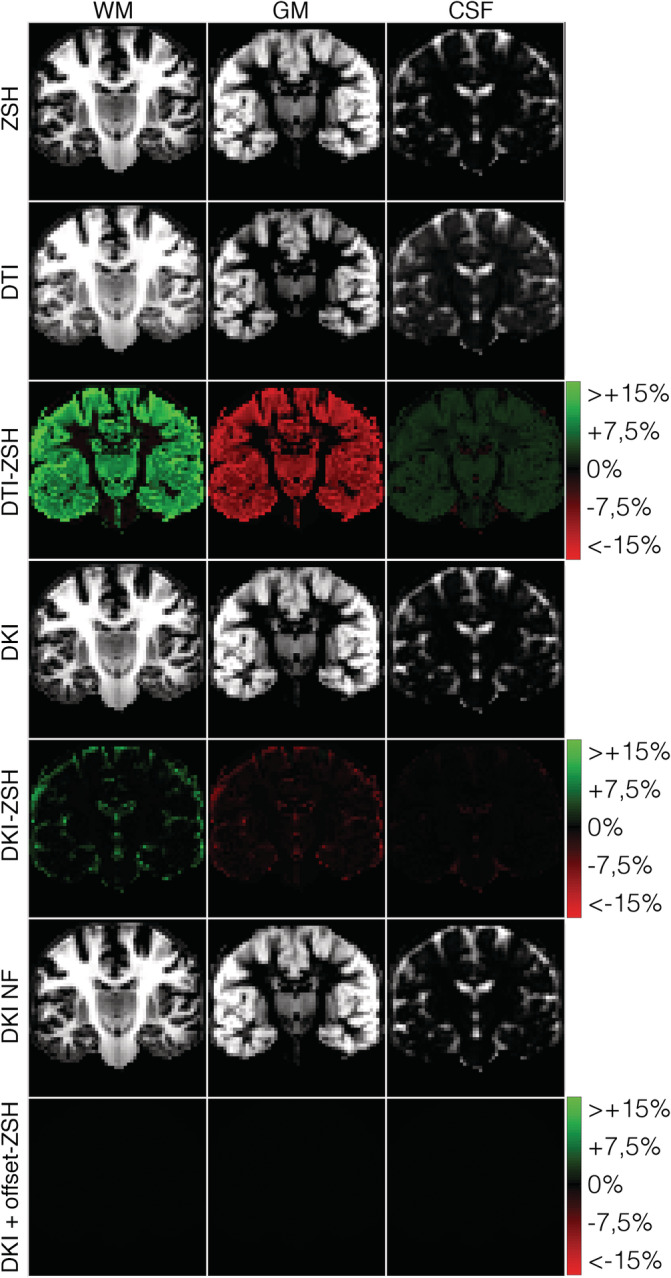
Relative differences (%) between the apparent densities obtained with the candidate response models and those obtained with the zonal spherical harmonics (ZSH) model on data set 1a

FIGURE 8.

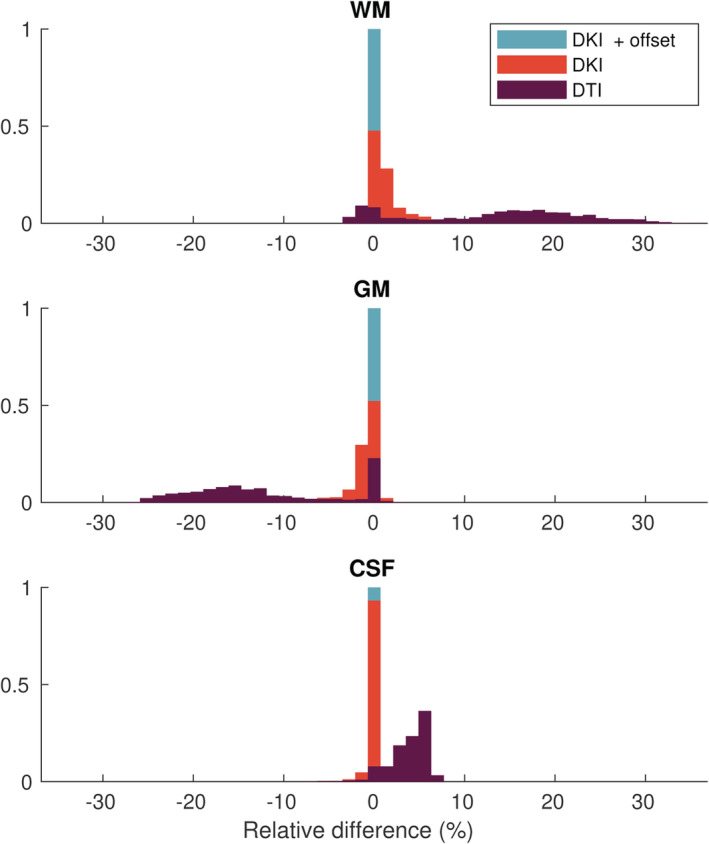
Histogram of the relative differences across the brain (%) between the apparent densities obtained with the candidate response models and those obtained with the zonal spherical harmonics (ZSH) model on data set 1a

When using the DTI models, in voxels predominantly containing CSF, the densities of CSF and GM are underestimated down to −3 and −5%, respectively, and WM densities are overestimated up to 13%. In voxels containing mostly GM, the densities of CSF and WM are consistently overestimated up to 7 and 32%, respectively, whereas the density of GM is underestimated down to −26%. In voxels containing predominantly WM, the densities of WM and CSF are overestimated up to 25 and 6%, respectively, and GM densities are underestimated down to −23%.

For the DKI models, in voxels containing predominantly CSF, WM densities are overestimated up to 11%, whereas CSF and GM densities are underestimated down to −3 and −5%, respectively. In voxels containing mostly GM, WM densities are overestimated up to 14% and CSF and GM densities are underestimated down to −1 and − 10%, respectively. In voxels containing predominantly WM, WM densities are overestimated up to 3%, whereas CSF and GM densities are underestimated down to −0.5 and − 2%, respectively.

The tissue densities estimated with the proposed DKI + offset RFs exhibit no noticeable differences throughout the brain (less than 0.1%) with those estimated using the state‐of‐the‐art ZSH.

Figure 9 shows the angular deviation of the largest fODF peak obtained with the candidate response models from that obtained with the ZSH model. When using the DTI model, considerable deviations up to 20° can be observed. Note that these large deviations occur primarily in voxels with partial volume effect between tissue types. These deviations reduced considerably when using the DKI model, with deviations mostly associated to voxels with CSF partial volume effect. The angular deviations of the peaks obtained with the DKI + offset model were less than 0,3°.

FIGURE 9.

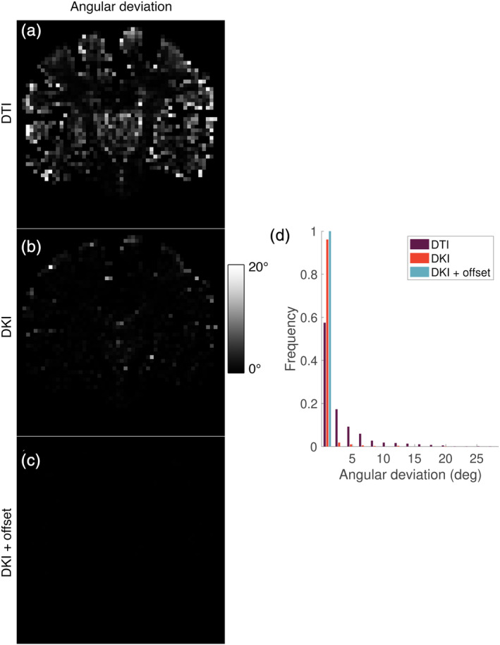
(a–c) Angular deviation (in degrees) of the largest fiber orientation density function (fODF) peak obtained with the candidate response models from that obtained with the zonal spherical harmonics (ZSH) model and (d) distribution of the deviations depicted in Figure 9a–c

Figure 10 shows the deviation of the amount of peaks obtained with the candidate models from those obtained with the state‐of‐the‐art ZSH model. When using the DTI model, the amount of peaks are underestimated by 1 in 0.2% of the voxels, overestimated by 1 in 27% of the voxels, and overestimated by 2 in 8% of the voxels. When using the DKI model, the amount of peaks are underestimated by −1 in 0.3% of the voxels, overestimated by 1 in 3% of the voxels, and overestimated by 2 in 0% of the voxels. When using the DKI + offset model, almost no deviations existed compared to the ZSH model.

FIGURE 10.

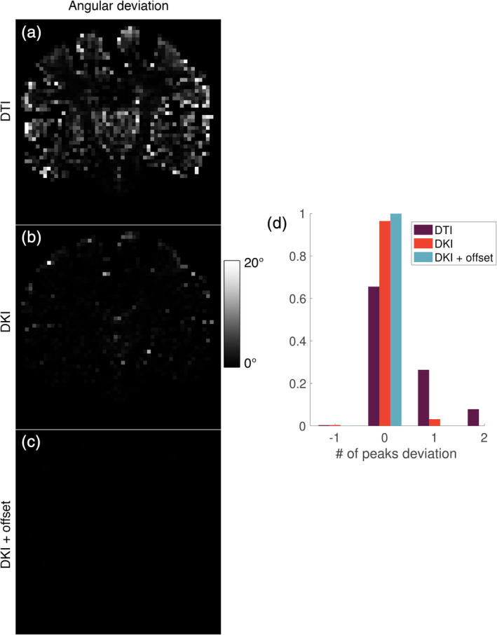
(a–c) Deviation of the amount of fiber orientation density function (fODF) peaks obtained with the candidate response models from those obtained with the zonal spherical harmonics (ZSH) model and (d) distribution of the deviations depicted in Figure 10a–c

4.2. Generalizability to higher b‐values

Figure 11 shows the comparison of the DKI + offset and ZSH models in the radial domain up to b = 10,000 s/mm². The signal predicted by the proposed model (which models also the radial dependency), closely matches the signal predicted by the ZSH model (which is performed per shell, effectively not modeling the radial dependency).

FIGURE 11.

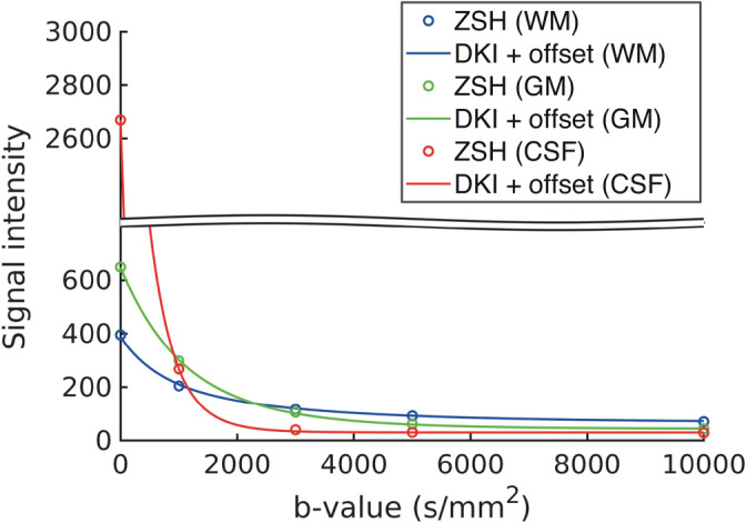
Generalizability to high b‐values: comparison of the radial component of tissue responses predicted by the diffusion kurtosis imaging (DKI) + offset model and those predicted by the zonal spherical harmonics (ZSH) for data set 3 with b‐values up to b = 10,000 s/mm²

4.3. Nonspherically sampled data experiments

4.3.1. Cartesian sampling

Figures 12 and 13 depict the signal responses predicted by the DKI + offset model, estimated with both the spherically (data set 1a) and Cartesian sampled data sets (data set 1b). Figure 12 shows the predicted signal response in the radial domain. As a reference, the signal predicted by the ZSH from data set 1a is also shown. Figure 13 shows the estimated WM signal response in the angular domain, including the signal predicted by the ZSH. The estimated signal responses remained the same when either a spherical or Cartesian sampling scheme were used.

FIGURE 12.

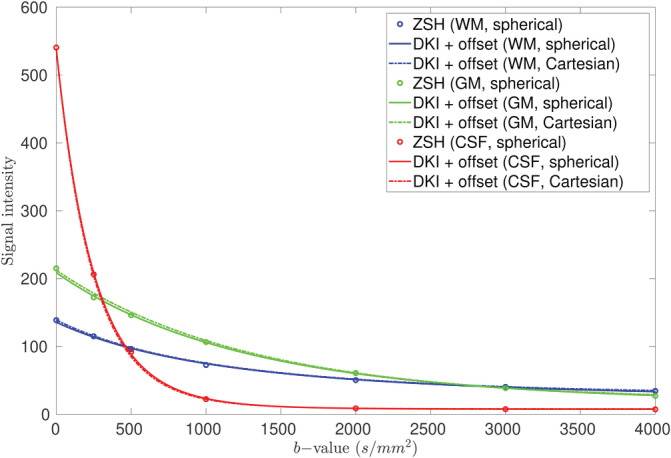
Comparison between the radial component of the tissue responses predicted by the diffusion kurtosis imaging (DKI) + offset using the spherically sampled data set (full lines), those predicted by the DKI + offset using the Cartesian sampled data set (dashed lines), and those predicted by the zonal spherical harmonics (ZSH) model using the spherically sampled data set (dots)

FIGURE 13.

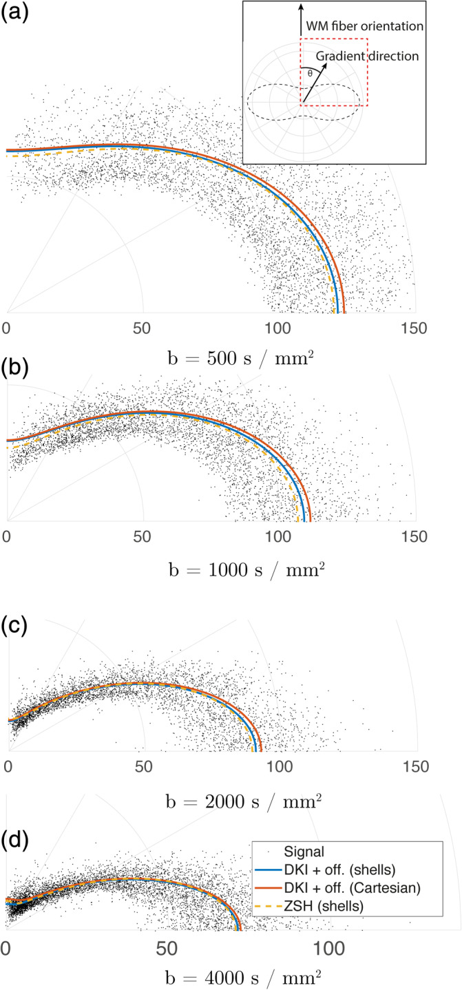
Comparison between the angular component of the white matter (WM) responses predicted by the diffusion kurtosis imaging (DKI) + offset using the spherically sampled data set, those predicted by the DKI + offset using the Cartesian sampled data set, and those predicted by the zonal spherical harmonics (ZSH) model using the spherically sampled data set, for various b‐values

Figure 14 demonstrates the application of MT‐SD to a Cartesian sampled data set with the DKI + offset RFs. The tissue densities that are estimated from data set 1b are very close to those estimated from data set 1a with the state‐of‐the‐art ZSH.

FIGURE 14.

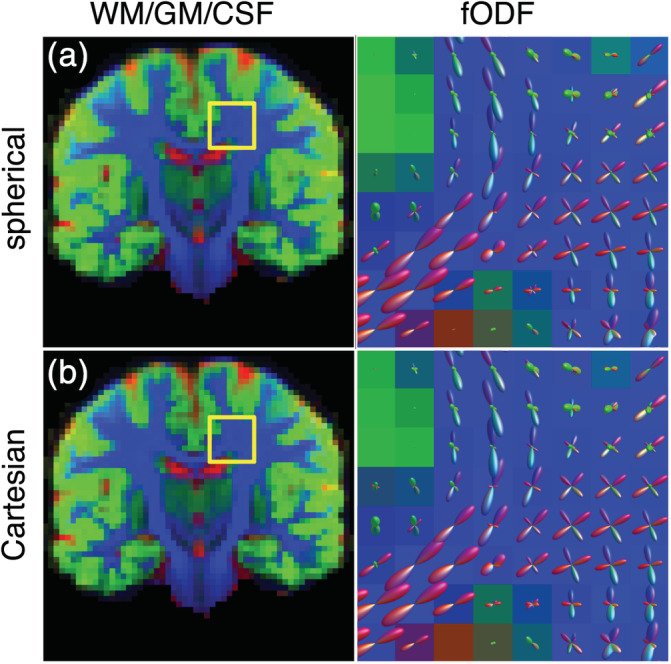
Comparison of the apparent densities (left) and the fiber orientation density functions (fODFs) (right) obtained with the diffusion kurtosis imaging (DKI) + offset model using both spherically sampled data (a) and Cartesian sampled data (b). The apparent densities are shown as RGB maps: cerebrospinal fluid (CSF) (red), gray matter (GM) (green), and white matter (WM) (blue)

4.3.2. Spherical sampling with gradient nonlinearities

MT‐SD was performed on data set 2 using the DKI + offset response model, both with and without taking into account the gradient nonlinearities. Figure 15 shows that the estimated tissue densities were biased up to +34% for WM and −25% for GM in areas where the nonlinearities are the most severe, with a lesser but still noticeable effect on CSF densities. Figure 16 shows the histogram of these differences across the whole brain.

FIGURE 15.

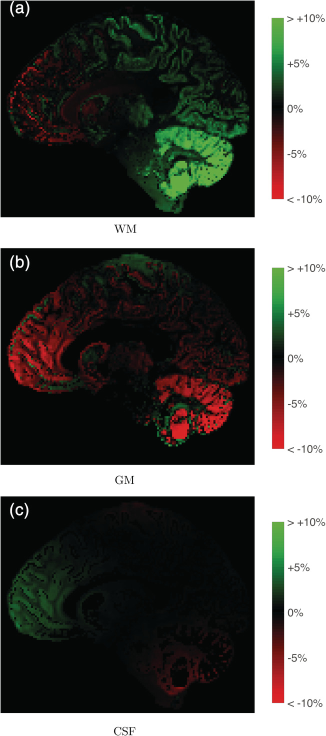
The effect of gradient nonlinearities on the apparent tissue densities obtained with multitissue‐spherical deconvolution (MT‐SD): relative errors of tissue densities (%) when not taking into account the gradient nonlinearities in the diffusion kurtosis imaging (DKI) + offset model. The values in the whole brain range between −10 and +34% for WM, between −25 and +12% for gray matter (GM), and between −6% and +6% for cerebrospinal fluid (CSF)

FIGURE 16.

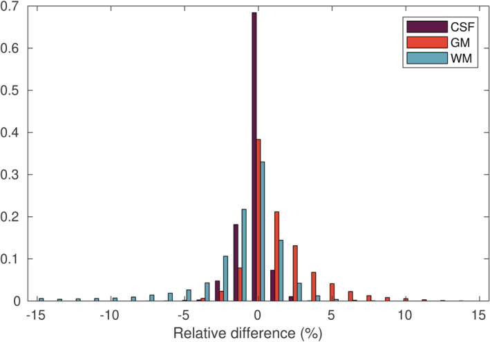
The effect of gradient nonlinearities on the apparent tissue densities obtained with multitissue‐spherical deconvolution (MT‐SD): histogram of the relative errors in apparent tissue densities across the brain (%) in data set 2, when not taking into account the gradient nonlinearities in the diffusion kurtosis imaging (DKI) + offset model. The values in the whole brain range between −10 and+34% for WM, between −25 and +12% for gray matter (GM), and between −6 and +6% for cerebrospinal fluid (CSF)

Figure 17 shows the relative connectivity bias of each brain parcel when not taking into account gradient nonlinearities. While the orientation and shape of the fODFs was largely unaffected by the gradient nonlinearities, the bias in densities caused large differences in the total “connectivity strengths” of each brain parcel, with relative differences of up to +7% in the cerebellum and down to −15% in the frontal lobe.

FIGURE 17.

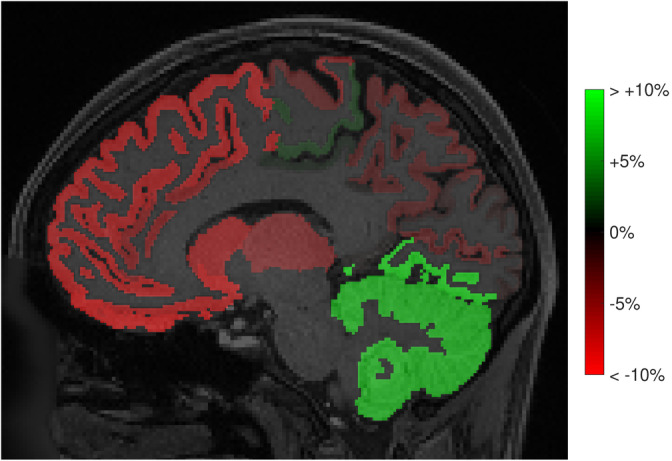
The effect of gradient nonlinearities on connectivity measures obtained with whole‐brain fiber tracking: relative errors in total connectivity of each parcel to all other parcels (%), when not taking into account the gradient nonlinearities in the diffusion kurtosis imaging (DKI) + offset model. The values in the whole brain ranged from −15 to +9%

5. DISCUSSION

In this work, we adopted a compact RF model for the purpose of (MT) SD that, in addition to the angular dependency, also describes the radial dependency. This allows MT‐SD of nonspherically sampled DW‐MRI data.

In the past, a second‐order tensor model has been used to represent tissue responses (Anderson, 2005; Dell'Acqua et al., 2007). Such a model can be evaluated at arbitrary b‐values, potentially enabling MT‐SD of nonspherically sampled DW‐MRI data. However, in this work we showed that this model is not compatible with high b‐value data sets typically used for SD (see Figures 3b,c and 4). Indeed, at higher b‐values, the signal decay is no longer monoexponential, and a higher‐order tensor model is required. To address this issue, we developed a RF model based on DKI, which can accurately describe the WM and GM responses across b‐values.

At high b‐values, we observed a nondecaying component in the CSF response, which cannot be described by the DKI model. As DW‐MRI data is generally noncentral chi distributed (den Dekker & Sijbers, 2014), for low signal to noise ratios, even if all of the true signal has decayed, there will still be a nonzero‐mean signal (Jones & Basser, 2004). Including an additional offset parameter allowed the accurate prediction of the CSF response (see Figure 3c). For WM and GM, this parameter only marginally improved the description of the signal (see Figure 5). However, at low signal‐to‐noise ratios, this parameter could become important to account for the noise floor in GM and WM as well. Note that, in the case of WM and GM, the offset parameter could also account for a nondecaying component caused by trapped water (Jbabdi, Sotiropoulos, Savio, Graña, & Behrens, 2012).

To reduce the complexity of the full DKI model (including the offset), we imposed axial symmetry around a known axis (in the case of WM), or isotropic diffusion (in the case of CSF and GM). This reduced the number of parameters from 23 to 7 and 4, respectively, enabling a very compact representation of the tissue responses across b‐values. In contrast, the state‐of‐the‐art approach which estimates the RF per shell using the ZSH basis functions requires 5 (l _max = 8) and 1 (l _max = 0) parameters per shell to model WM and GM/CSF, respectively. Despite the low number of parameters, the proposed model provides signal responses almost equivalent to the state‐of‐the‐art ZSH.

5.1. Implications of using an inappropriate response model

The use of an inappropriate model for the MT RFs can severely bias the resulting apparent tissue densities. As Figure 7 shows, there are systematic deviations in the densities across the entire brain when a second‐order model is used to describe tissue responses. Because the DTI AS model severely underestimates the WM signal for b‐values exceeding b = 1,000 s/mm², the WM densities can exhibit a bias of up to +32% in voxels containing multiple tissue types, especially near WM/GM interfaces. Conversely, the GM densities are underestimated down to −26% (see Figure 8). When employing the fourth‐order models, these deviations are greatly reduced, but are still visible in voxels containing CSF. By adding the offset parameter, these deviations are reduced below 0.1%, as the CSF response is now modeled accurately (see Figure 3c).

5.2. Generalizability to higher b‐values

The proposed model is based on a Taylor series expansion about b = 0 s/mm². This means that it only provides an accurate approximation for b‐values in the vicinity of b = 0 s/mm², potentially invalidating the model at very high b‐values. However, using a dMRI data set with b‐values as high as b = 10,000 s/mm², we demonstrated that it is able to closely predict MT signal responses across the entire b‐value range. While this does not completely rule out potential issues, it demonstrates that the proposed model is able to accommodate also more exotic data sets featuring high b‐values with a large degree of accuracy.

5.3. Implications for nonspherically sampled data

The ZSH coefficients cannot be estimated directly from nonspherically sampled data, as they only describe the angular dependency of the tissue responses. In contrast, the parameters of the proposed response model are estimated using all DW measurements simultaneously and allow the accurate description of the signal for a continuous range of b‐values. As a result, our approach facilitates (MT) SD analysis of a much broader range of nonspherically sampled data sets, such as DSI.

5.4. Implications for data affected by gradient nonlinearities

Nonspherical sampling cannot only be intrinsic to the DW scheme, but the result of gradient nonlinearities as well. Due to this, the true b‐values can deviate significantly from their assumed values (see Figure 2), and they cannot be accounted for if the RF is estimated per shell. As a consequence, the apparent tissue densities can be biased as much as 34% (see Figures 15 and 16). Using the proposed approach, gradient nonlinearities can be accounted for, resulting in much more accurate apparent tissue densities. This could benefit studies employing apparent tissue densities obtained from data acquired with strong gradient amplitudes (Calamante, Jeurissen, Smith, Tournier, & Connelly, 2018; Chamberland et al., 2019; St‐Jean, Chamberland, Viergever, & Leemans, 2019).

5.5. Implications for downstream processing

Biases in the fODF, either due to an inappropriate response model or as a result of gradient nonlinearities, can have implications for any methods and studies that use fODF‐based metrics. The fODF amplitude or AFD, which is used as a marker for intra‐axonal volume fraction will be biased, complicating biological interpretation and potentially leading to misleading findings (see Figures 6, 7, 8 and 15). Fiber tracking is also sensitive to such biases as it typically employs an fODF amplitude threshold as a termination criterion. As such, biased fODF amplitudes can lead to streamlines ending prematurely or too far into the cortex (Jeurissen et al., 2014). Furthermore, quantitative tractography approaches such as SIFT employ the fiber densities to improve the fit between the streamline reconstruction and the underlying DW images (Smith, Tournier, Calamante, & Connelly, 2013). As the proposed method can provide more accurate apparent fiber densities in the presence of significant gradient nonlinearities, it will directly improve the quantitative nature of tractography and connectomics studies employing SD in combination with high gradient strengths (Roine et al., 2019). Indeed, considerable changes in connectivity (up to +9% and down to −15%) were observed as a consequence of gradient nonlinearities, which are accounted for with the proposed method. In light of the implications mentioned above, we encourage always accounting for gradient nonlinearities when working with HCP data (Mesri et al., 2019).

5.6. Potential bias due to intravoxel incoherent motion effects at low b‐values

A potential limitation of the proposed model is that for data acquired with b‐values ranging between 0 and 500 s/mm², intravoxel incoherent motion or free water effects might come into play. The proposed response model might no longer be appropriate, and the addition of an additional second‐order compartment corresponding to fast diffusion could improve the signal prediction across all b‐values.

6. CONCLUSION

We adopted a model for tissue responses that describes both the angular and radial dependencies. Currently, the state‐of‐the‐art ZSH basis functions only describe the signal in the angular domain, which precludes (MT) SD analysis of nonspherically sampled data sets. In addition, DTI‐based models are incapable of describing the signal across a wide range of b‐values, whereas the proposed model provides responses equivalent to the state of the art. Because of the continuous representation of the signal in the radial domain, a broader range of (nonspherically sampled) DW data sets can be processed using (MT) SD. In addition, gradient nonlinearities can be accounted for, allowing more accurate downstream processing.

CONFLICT OF INTEREST

The authors declare no conflicts of interest.

The components $T_{j_1{j}_2\dots j_n}^{i_1{i}_2\dots i_m}$ of an (m, n) tensor T transform between two coordinate systems (denoted by the primed and unprimed indices) according to the tensor transformation law (using the Einstein‐summation convention):

$$T_{j_1^{\prime }{j}_2^{\prime }\cdots j_n^{\prime }}^{i_1^{\prime }{i}_2^{\prime }\cdots i_m^{\prime }}=R_{i_1}^{i_1^{\prime }}\dots R_{i_m}^{i_m^{\prime }}{R}_{j_1^{\prime }}^{j_1}\dots R_{j_n^{\prime }}^{j_n}{T}_{j_1{j}_2\cdots j_n}^{i_1{i}_2\cdots i_m}$$ (A1)

The factors $R_k^{k^{\prime }}$ are the partial derivatives of the coordinate transform x ^k′(x ^k):

$$R_k^{k^{\prime }}=\frac{\partial x^{k^{\prime }}}{\partial x^k}$$

This transformation law can be exploited to find the relations between the components of a tensor subject to specific spatial symmetries. In this case, to find the components of an axially symmetric tensor aligned along the z‐axis, we choose a rotation about the z‐axis. The indices 1, 2, and 3 correspond to the x, y, and z‐axes, respectively. The coordinate transform can then be written as:

$$\begin{array}{l}{x}^{1^{\prime }}=x^1\cos \theta +x^2\sin \theta \\ x^{2^{\prime }}=-x^1\sin \theta +x^2\cos \theta \\ x^{3^{\prime }}=x^3\end{array}$$

Or more compactly:

$$x^{k^{\prime }}=R_k^{k^{\prime }}{x}^k$$

For θ small, we can use a first‐order Taylor approximation for the trigonometric functions and write (Jeffreys, 1931):

$$R_k^{k^{\prime }}\approx {\delta }_k^{k^{\prime }}+c_k^{k^{\prime }}$$ (A2)

with ${\delta }_k^{k^{\prime }}$ the Kronecker delta and $c_k^{k^{\prime }}$ hollow and antisymmetric:

$$c_k^{k^{\prime }}=\left(\begin{array}{lll}0& \theta & 0\\ -\theta & 0& 0\\ 0& 0& 0\end{array}\right)$$

Applying the tensor transformation law (A1) to a fourth‐order tensor W and using expression (A2) results in:

$$\begin{array}{l}{W}_{\mathit{\text{ijkl}}}=W_{i^{\prime }{j}^{\prime }{k}^{\prime }{l}^{\prime }}\\ +c_{i^{\prime }i}{W}_{i{j}^{\prime }{k}^{\prime }{l}^{\prime }}+c_{j^{\prime }j}{W}_{i^{\prime }j{k}^{\prime }{l}^{\prime }}+c_{k^{\prime }k}{W}_{i^{\prime }{j}^{\prime }k{l}^{\prime }}+c_{l^{\prime }l}{W}_{i^{\prime }{j}^{\prime }{k}^{\prime }l}\end{array}$$ (A3)

Demanding that W is invariant means that the coordinate transformation does not affect its components:

$$W_{i^{\prime }{j}^{\prime }{k}^{\prime }{l}^{\prime }}=W_{\mathit{\text{ijkl}}}$$ (A4)

Combining Equations (A3) and (A4), this implies:

$$c_{i^{\prime }i}{W}_{i{j}^{\prime }{k}^{\prime }{l}^{\prime }}+c_{j^{\prime }j}{W}_{i^{\prime }j{k}^{\prime }{l}^{\prime }}+c_{k^{\prime }k}{W}_{i^{\prime }{j}^{\prime }k{l}^{\prime }}+c_{l^{\prime }l}{W}_{i^{\prime }{j}^{\prime }{k}^{\prime }l}=0$$ (A5)

Checking Equation (A5) for all possible (i′, j′, k′, l′) tuples will result in restrictions on the components of W _ijkl. For example, choosing the tuple (1, 2, 3, 3) and assuming that W is fully symmetric in all of its indices implies the following restriction:

$$W_{2233}=W_{1133}$$ (A6)

In an analogous way, we find an additional restriction:

$$3W_{1122}=W_{1111}=W_{2222}$$ (A7)

For the component W ₃₃₃₃, no restrictions are found, which means that it is an independent component.

Morez J, Sijbers J, Vanhevel F, Jeurissen B. Constrained spherical deconvolution of nonspherically sampled diffusion MRI data. Hum Brain Mapp. 2021;42:521–538. 10.1002/hbm.25241

DATA AVAILABILITY STATEMENT

The data that support the findings of this study are available from the corresponding author upon reasonable request.

REFERENCES

- Alexander, D. C. , Hubbard, P. L. , Hall, M. G. , Moore, E. A. , Ptito, M. , Parker, G. J. M. , & Dyrby, T. B. (2010). Orientationally invariant indices of axon diameter and density from diffusion MRI. NeuroImage, 52(4), 1374–1389. [DOI] [PubMed] [Google Scholar]
- Anderson, A. W. (2005). Measurement of fiber orientation distributions using high angular resolution diffusion imaging. Magnetic Resonance in Medicine, 54(5), 1194–1206. [DOI] [PubMed] [Google Scholar]
- Bai, Y. , & Alexander, D. C. (2008). Model‐based registration to correct for motion between acquisitions in diffusion mr imaging. In 2008 5th IEEE International Symposium on Biomedical Imaging: From Nano to Macro .
- Bammer, R. , Markl, M. , Barnett, A. , Acar, B. , Alley, M. , Pelc, N. , … Moseley, M. (2003). Analysis and generalized correction of the effect of spatial gradient field distortions in diffusion‐weighted imaging. Magnetic Resonance in Medicine, 50(3), 560–569. [DOI] [PubMed] [Google Scholar]
- Baron, C. A. , Lebel, R. M. , Wilman, A. H. , & Beaulieu, C. (2012). The effect of concomitant gradient fields on diffusion tensor imaging. Magnetic Resonance in Medicine, 68(4), 1190–1201. [DOI] [PubMed] [Google Scholar]
- Borkowski, K. , & KrzyŻak, A. T. (2018). Analysis and correction of errors in DTI‐based tractography due to diffusion gradient inhomogeneity. Journal of Magnetic Resonance, 296, 5–11. [DOI] [PubMed] [Google Scholar]
- Burnham, K. P. , & Anderson, D. R. (1998). Model selection and multimodel inference: A practical information‐theoretic approach. New York, NY: Springer‐Verlag. [Google Scholar]
- Calamante, F. , Jeurissen, B. , Smith, R. E. , Tournier, J.‐D. , & Connelly, A. (2018). The role of whole‐brain diffusion MRI as a tool for studying human in vivo cortical segregation based on a measure of neurite density. Magnetic Resonance in Medicine, 79(5), 2738–2744. [DOI] [PubMed] [Google Scholar]
- Chamberland, M. , Raven, E. P. , Genc, S. , Duffy, K. , Descoteaux, M. , Parker, G. D. , … Jones, D. K. (2019). Dimensionality reduction of diffusion MRI measures for improved tractometry of the human brain. NeuroImage, 200, 89–100. [DOI] [PMC free article] [PubMed] [Google Scholar]
- Christiaens, D. , Sunaert, S. , Suetens, P. , & Maes, F. (2017). Convexity‐constrained and nonnegativity‐constrained spherical factorization in diffusion‐weighted imaging. NeuroImage, 146, 507–517. [DOI] [PMC free article] [PubMed] [Google Scholar]
- Dell'Acqua, F. , Rizzo, G. , Scifo, P. , Clarke, R. A. , Scotti, G. , & Fazio, F. (2007). A model‐based deconvolution approach to solve fiber crossing in diffusion‐weighted MR imaging. IEEE Transactions on Biomedical Engineering, 54(3), 462–472. [DOI] [PubMed] [Google Scholar]
- Dell'Acqua, F. , & Tournier, J. D. (2019). Modelling white matter with spherical deconvolution: How and why? NMR in Biomedicine, 32(4), e3945. [DOI] [PMC free article] [PubMed] [Google Scholar]
- den Dekker, A. J. , & Sijbers, J. (2014). Data distributions in magnetic resonance images: A review. Physica Medica, 30(7), 725–741. [DOI] [PubMed] [Google Scholar]
- Desikan, R. S. , Ségonne, F. , Fischl, B. , Quinn, B. T. , Dickerson, B. C. , Blacker, D. , … Killiany, R. J. (2006). An automated labeling system for subdividing the human cerebral cortex on MRI scans into gyral based regions of interest. NeuroImage, 31(3), 968–980. [DOI] [PubMed] [Google Scholar]
- Ferizi, U. , Schneider, T. , Panagiotaki, E. , Nedjati‐Gilani, G. , Zhang, H. , Wheeler‐Kingshott, C. A. M. , & Alexander, D. C. (2014). A ranking of diffusion MRI compartment models with in vivo human brain data. Magnetic Resonance in Medicine, 72(6), 1785–1792. [DOI] [PMC free article] [PubMed] [Google Scholar]
- Glasser, M. F. , Sotiropoulos, S. N. , Wilson, J. A. , Coalson, T. S. , Fischl, B. , Andersson, J. L. , … WU‐Minn HCP Consortium . (2013). The minimal preprocessing pipelines for the Human Connectome Project. NeuroImage, 80, 105–124. [DOI] [PMC free article] [PubMed] [Google Scholar]
- Guo, F. , Leemans, A. , Viergever, M. A. , Dell'Acqua, F. , & de Luca, A. (2020). Generalized Richardson‐lucy (grl) for analyzing multi‐shell diffusion MRI data. NeuroImage, 218, 116948. [DOI] [PubMed] [Google Scholar]
- Hansen, B. , Shemesh, N. , & Jespersen, S. N. (2016). Fast imaging of mean, axial and radial diffusion kurtosis. NeuroImage, 142, 381–393. [DOI] [PMC free article] [PubMed] [Google Scholar]
- Jbabdi, S. , Sotiropoulos, S. N. , Savio, A. M. , Graña, M. , & Behrens, T. E. J. (2012). Model‐based analysis of multishell diffusion MR data for tractography: How to get over fitting problems. Magnetic Resonance in Medicine, 68(6), 1846–1855. [DOI] [PMC free article] [PubMed] [Google Scholar]
- Jeffreys, H. (1931). Cartesian tensors, Cambridge: Cambridge University Press. [Google Scholar]
- Jensen, J. H. , & Helpern, J. A. (2010). MRI quantification of non‐Gaussian water diffusion by kurtosis analysis. NMR in Biomedicine, 23(7), 698–710. [DOI] [PMC free article] [PubMed] [Google Scholar]
- Jeurissen, B. , Descoteaux, M. , Mori, S. , & Leemans, A. (2019). Diffusion MRI fiber tractography of the brain. NMR in Biomedicine, 32(4), e3785. [DOI] [PubMed] [Google Scholar]
- Jeurissen, B. , Tournier, J. D. , Dhollander, T. , Connelly, A. , & Sijbers, J. (2014). Multi‐tissue constrained spherical deconvolution for improved analysis of multi‐shell diffusion MRI data. NeuroImage, 103, 411–426. [DOI] [PubMed] [Google Scholar]
- Jones, D. , Horsfield, M. , & Simmons, A. (1999). Optimal strategies for measuring diffusion in anisotropic systems by magnetic resonance imaging. Magnetic Resonance in Medicine, 42(3), 515–525. [PubMed] [Google Scholar]
- Jones, D. K. , & Basser, P. J. (2004). "Squashing peanuts and smashing pumpkins": How noise distorts diffusion‐weighted MR data. Magnetic Resonance in Medicine, 52(5), 979–993. [DOI] [PubMed] [Google Scholar]
- Kaden, E. , Knösche, T. R. , & Anwander, A. (2007). Parametric spherical deconvolution: Inferring anatomical connectivity using diffusion MR imaging. NeuroImage, 37(2), 474–488. [DOI] [PubMed] [Google Scholar]
- Kellner, E. , Dhital, B. , & Reisert, M. (2016). Gibbs‐ringing artifact removal based on local. Magnetic Resonance in Medicine, 76, 1574–1581. [DOI] [PubMed] [Google Scholar]
- Mesri, H. Y. , David, S. , Viergever, M. A. , & Leemans, A. (2020). The adverse effect of gradient nonlinearities on diffusion MRI: From voxels to group studies. NeuroImage, 205, 116127 10.1016/j.neuroimage.2019.116127 [DOI] [PubMed] [Google Scholar]
- Moseley, M. E. , Cohen, Y. , Kucharczyk, J. , Mintorovitch, J. , Asgari, H. , Wendland, M. , … Norman, D. (1990). Diffusion‐weighted mr imaging of anisotropic water diffusion in cat central nervous system. Radiology, 176(2), 439–445. [DOI] [PubMed] [Google Scholar]
- Özarslan, E. , Koay, C. G. , & Basser, P. J. (2013). Simple harmonic oscillator based reconstruction and estimation for one‐dimensional q‐space magnetic resonance (1d‐shore) In Andrews T. D., Balan R., Benedetto J. J., Czaja W., & Okoudjou K. A. (Eds.), Excursions in harmonic analysis, volume 2: The February Fourier talks at the Norbert Wiener Center (pp. 373–399). Boston, MA: Birkhäuser Boston. [Google Scholar]
- Roine, T. , Jeurissen, B. , Perrone, D. , Aelterman, J. , Philips, W. , Sijbers, J. , & Leemans, A. (2019). Reproducibility and intercorrelation of graph theoretical measures in structural brain connectivity networks. Medical Image Analysis, 52, 56–67. [DOI] [PubMed] [Google Scholar]
- Scherrer, B. , & Warfield, S. K. (2012). Parametric representation of multiple white matter fascicles from cube and sphere diffusion MRI. PLoS One, 7(11), e48232. [DOI] [PMC free article] [PubMed] [Google Scholar]
- Smith, R. E. , Tournier, J. D. , Calamante, F. , & Connelly, A. (2013). SIFT: Spherical‐deconvolution informed filtering of tractograms. NeuroImage, 67, 298–312. [DOI] [PubMed] [Google Scholar]
- Smith, R. E. , Tournier, J.‐D. , Calamante, F. , & Connelly, A. (2015). Sift2: Enabling dense quantitative assessment of brain white matter connectivity using streamlines tractography. NeuroImage, 119, 338–351. [DOI] [PubMed] [Google Scholar]
- Sotiropoulos, S. N. , Jbabdi, S. , Xu, J. , Andersson, J. L. , Moeller, S. , Auerbach, E. J. , … Behrens, T. E. J. (2013). Advances in diffusion MRI acquisition and processing in the Human Connectome Project. NeuroImage, 80, 125–143. [DOI] [PMC free article] [PubMed] [Google Scholar]
- Stejskal, E. O. , & Tanner, J. E. (1965). Spin diffusion measurements: Spin echoes in the presence of a time‐dependent field gradient. The Journal of Chemical Physics, 42(1), 288–292. [Google Scholar]
- St‐Jean, S. , Chamberland, M. , Viergever, M. A. , & Leemans, A. (2019). Reducing variability in along‐tract analysis with diffusion profile realignment. NeuroImage, 199, 663–679. [DOI] [PubMed] [Google Scholar]
- Tabesh, A. , Jensen, J. H. , Ardekani, B. A. , & Helpern, J. A. (2011). Estimation of tensors and tensor‐derived measures in diffusional kurtosis imaging. Magnetic Resonance in Medicine, 65(3), 823–836. [DOI] [PMC free article] [PubMed] [Google Scholar]
- Tax, C. M. , Jeurissen, B. , Vos, S. B. , Viergever, M. A. , & Leemans, A. (2014). Recursive calibration of the fiber response function for spherical deconvolution of diffusion MRI data. NeuroImage, 86, 67–80. [DOI] [PubMed] [Google Scholar]
- Tournier, J. D. , Calamante, F. , & Connelly, A. (2007). Robust determination of the fibre orientation distribution in diffusion MRI: Non‐negativity constrained super‐resolved spherical deconvolution. NeuroImage, 35(4), 1459–1472. [DOI] [PubMed] [Google Scholar]
- Tournier, J. D. , Calamante, F. , & Connelly, A. (2013). Determination of the appropriate b value and number of gradient directions for high‐angular‐resolution diffusion‐weighted imaging. NMR in Biomedicine, 26(12), 1775–1786. [DOI] [PubMed] [Google Scholar]
- Tournier, J.‐D. , Calamante, F. , & Connelly, A. (2010). Improved probabilistic streamlines tractography by 2nd order integration over fibre orientation distributions. ISMRM, 18, 1670. [Google Scholar]
- Tournier, J. D. , Calamante, F. , Gadian, D. G. , & Connelly, A. (2004). Direct estimation of the fiber orientation density function from diffusion‐weighted MRI data using spherical deconvolution. NeuroImage, 23(3), 1176–1185. [DOI] [PubMed] [Google Scholar]
- Tournier, J. D. , Smith, R. , Raffelt, D. , Tabbara, R. , Dhollander, T. , Pietsch, M. , … Connelly, A. (2019). MRtrix3: A fast, flexible and open software framework for medical image processing and visualisation. NeuroImage, 202, 116137 10.1016/j.neuroimage.2019.116137 [DOI] [PubMed] [Google Scholar]
- Tustison, N. J. , Avants, B. B. , Cook, P. A. , Zheng, Y. , Egan, A. , Yushkevich, P. A. , & Gee, J. C. (2010). N4ITK: Improved N3 bias correction. IEEE Transactions on Medical Imaging, 29(6), 1310–1320. [DOI] [PMC free article] [PubMed] [Google Scholar]
- Veraart, J. , Novikov, D. S. , Christiaens, D. , Ades‐Aron, B. , Sijbers, J. , & Fieremans, E. (2016). Denoising of diffusion MRI using random matrix theory. NeuroImage, 142, 394–406. [DOI] [PMC free article] [PubMed] [Google Scholar]
- Veraart, J. , Poot, D. H. J. , van Hecke, W. , Blockx, I. , van der Linden, A. , Verhoye, M. , & Sijbers, J. (2011). More accurate estimation of diffusion tensor parameters using diffusion kurtosis imaging. Magnetic Resonance in Medicine, 65(1), 138–145. [DOI] [PubMed] [Google Scholar]
- Veraart, J. , Sijbers, J. , Sunaert, S. , Leemans, A. , & Jeurissen, B. (2013). Weighted linear least squares estimation of diffusion MRI parameters: Strengths, limitations, and pitfalls. NeuroImage, 81, 335–346. [DOI] [PubMed] [Google Scholar]
- Wedeen, V. J. , Hagmann, P. , Tseng, W.‐Y. I. , Reese, T. G. , & Weisskoff, R. M. (2005). Mapping complex tissue architecture with diffusion spectrum magnetic resonance imaging. Magnetic Resonance in Medicine, 54(6), 1377–1386. [DOI] [PubMed] [Google Scholar]
Associated Data
This section collects any data citations, data availability statements, or supplementary materials included in this article.