Neural Network Vessel Lumen Regression for Automated Lumen Cross-Section Segmentation in Cardiovascular Image-Based Modeling

Abstract

We accelerate a pathline-based cardiovascular model building method by training machine learning models to directly predict vessel lumen surface points from computed tomography (CT) and magnetic resonance (MR) medical image data. Formulating vessel lumen detection as a regression task using a polar coordiantes representation allows predictions to be made with significantly higher accuracy than existing methods that identify the vessel lumen through binary pixel classification. The regression formulation enables machine learning models to be trained end-to-end for vessel lumen detection without post-processing steps that reduce accuracy. By employing our models in a pathline-based cardiovascular model building pipeline we substantially reduce the manual segmentation effort required to build accurate cardiovascular models, and reduce the overall time required to perform patient-specific cardiovascular simulations. While our method is applied here for cardiovascular model building it is generally applicable to segmentation of tree-like and tubular structures from image data.

1. Introduction

The increasing worldwide prevalence of Cardiovascular disease (CVD) [13] has spurred the development of new computational cardiovascular modeling and simulation technologies [6]. Image-based patient-specific hemodynamic simulation methods, in particular, are used in personalized medicine and surgical planning for a range of disease applications [42,28].

However, the typically manual segmentation effort required to construct accurate 3D digital anatomical cardiovascular models for patient-specific hemodynamic simulations is currently a labor intensive and time consuming process [42,36]. Lengthy workflows are incompatible with realistic clinical settings where limited time is available to produce simulation results. Furthermore, to validate the efficacy of simulation tools, studies and trials involving large patient cohorts are required to statistically correlate simulation predictions with clinical outcomes, making lengthy workflows intractable.

Specialized software tools such as SimVascular¹ [43, 44], Cardiovascular Integrated Modeling and Simulation (CRIMSON) [18], and Vascular Modeling Toolkit (VMTK) [1] have been developed to provide hemodynamic simulation worfklows. With these software tools, users can construct 3D cardiovascular models vessel-by-vessel (Fig. 1). A recent framework based on isogeometric analysis enables construction of detailed cardiovasular models readily usable for simulations, but still relies on thresholding and manual user interaction to initialize the process with a cardiovascular segmentation [45]. While users can use the listed software packages to construct sufficiently accurate and precise cardiovascular models, they typically find the segmentation step to be cumbersome and time-consuming (Fig. 1c).

Fig. 1:

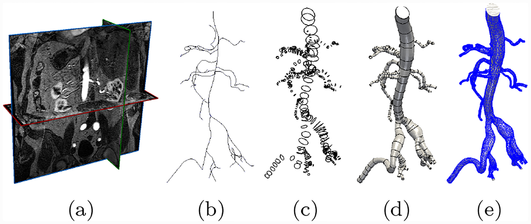
The cardiovascular model construction workflow used in SimVascular [43]. Starting from (a) Image data, (b) users manually generate pathlines, (c) use these pathlines to segment 2D cross section contours, (d) loft segmented contours into a 3D model, (e) generate a 3D geometric mesh for use in cardiovascular simulations.

Thus, there is a clear need for rapid and automated cardiovascular segmentation methods. Prior studies have been devoted to improving cardiovascular segmentation [25,37,35], but no commonly accepted methods exist that generalize to varying image modalities and cardiovascular anatomy. Initial approaches fall into the categories of active contours [46,26], vessel enhancement methods such as Hessian filtering [8] and Optimally Oriented Flux [22,23]. Stochastic random-walk based methods were also developed for tubular structure segmentation [10]. Other methods take advantage of the consistent shape and appearance of blood vessels, such as intensity models [21], 4D curves [3], cross-sectional approaches [39,20], image gradient methods [31], vessel templates [50] and vessel tracking [9]. The most recent methods are based on statistical techniques such as Random Sample Consensus (RANSAC)[17], and machine learning techniques [2,30]. Modern optimization algorithm based cardiovascular segmentation methods have also been developed [33]. However, a severe disadvantage of most segmentation algorithms, such as e.g. active contours, is the large number of input parameters they require. The time required to identify optimal values for input parameters is often prohibitive and therefore leads to little segmentation time savings. As a result, the need to tune parameters for each new patient case, modality, and anatomical region precludes the use of many automated segmentation algorithms for in hemodynamic simulation studies.

Recent developments in deep learning and computer vision suggest that convolutional neural networks (CNN), a type of neural network tailored to visual input data, present an avenue towards the development of more general segmentation algorithms [24,38,16,7,4,29,14]. The I2I [29] and DeepLumen networks [32] demonstrated state-of-the-art accuracy on cardiovascular edge detection and coronary artery segmentation respectively. In a previous study we investigated the use of fully convolutional neural networks (FCNN), trained for binary pixel classification, for cardiovascular patient-specific model construction [27]. Our FCNN approach improved segmentation accuracy over comparable threshold and level set methods. However, FCNNs can only segment structures that are clearly visible in the input image, this limitation lead to erroneous vessel lumen segmentation with input images with poor resolution or visibility of the target vessel, such as coronary arteries with substantial surrounding tissue.

Recent studies have demonstrated that neural network segmentation accuracy can be improved by directly predicting the boundary points of the structure of interest using a polar coordinates formulation, as opposed to binary labeling of pixels in the input image [32,48,49]. However, these studies were limited to natural images [49] and the coronary arteries [32,48]. In particular [48] used a ray-casting formulation which requires a-priori specification of a region of interest which is non-trivial to apply across different anatomical regions containing vessels with substantial radius variation.

In this work we significantly improve the accuracy of our previous cardiovascular model building method. We develop a convolutional neural network, that directly predicts vessel lumen points via a polar coordinates formulation. We then apply our CNN to accelerate a path-planning cardiovascular modeling method. Unlike previous studies, our CNN is applicable to both CT and MR modalities and generalizes across anatomical regions and vessel sizes.

We demonstrate the generality of our method on a dataset of mixed CT and MR medical image volumes spanning varying cardiovascular anatomical regions. Our CNN achieves accuracy comparable to average segmentation agreement between expert users of SimVascular as measured on segmentations produced for a MR cerebrovascular, pulmonary and coronary vasculature case and a CT abdominal aortic aneurysm case.

2. Methods

Our proposed CNN segmentation pipeline (Fig. 2), resembles the existing pathline-based model construction workflow of SimVascular. (Fig. 1). However, with our proposed pipeline, during the segmentation step, the extracted 2D images are preprocessed and input to a CNN that has been trained to directly predict the vessel lumen boundary points using a polar coordinates representation (Fig. 2b,c). This improves segmentation accuracy over typical approaches such as CNN pixel segmentation networks such as UNet and CENet [34,11], or level set algorithms, as examined in our previous work [27], in part because our approach avoids the need for additional image processing steps, e.g. marching-squares, to extract the lumen points. The final vessel lumen boundary is constructed by reorienting the produced lumen boundary points in 3D space and interpolating along the pathline. Merging the individual vessels with geometric boolean operations [44] produces the desired 3D patient-specific model.

Fig. 2:

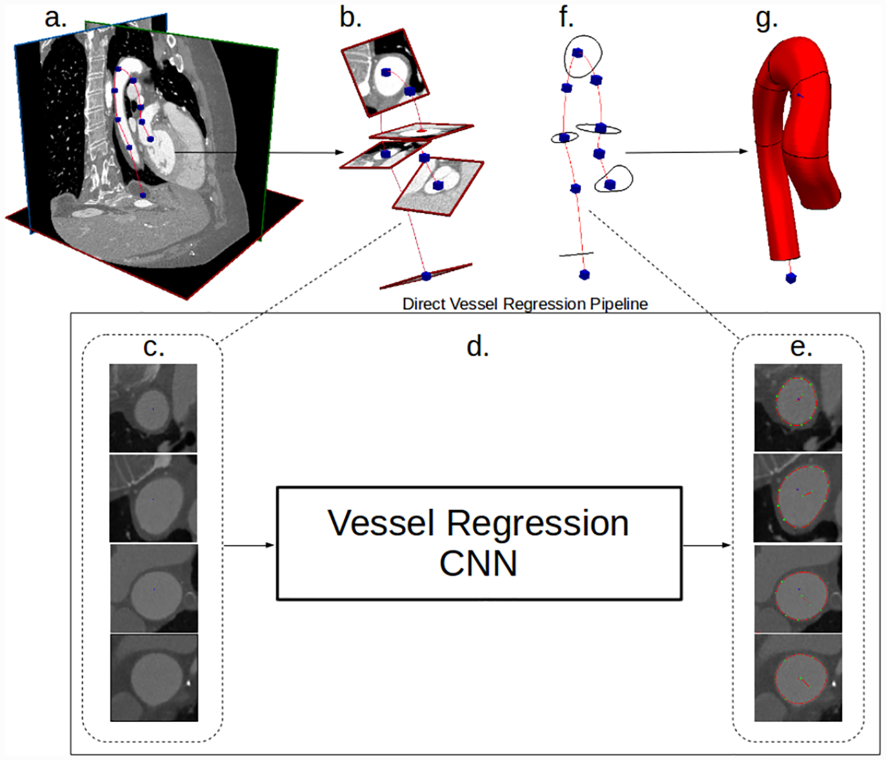
Our convolutional lumen regression network cardiovascular model building pipeline. (a) Image data and vessel pathline supplied by the user. (b) Path information is used to extract image pixel intensities in the plane perpendicular to the vessel path. (c) 2D images extracted along vessel pathlines are input to the CNN. (d) and (e) Our CNN processes the 2D vessel cross-section input images and directly outputs a vector of the lumen boundary points. (f) The 2D vessel lumen boundary points are transformed back to 3D space. (g) Cross-sectional vessel boundaries are interpolated in 3D space along the pathline to form the final vessel model.

We work within the cardiovascular modeling pipeline in the open source SimVascular package to demonstrate performance of our CNN. However, we note that the methods we present are generally applicable to other approaches which rely on the path-planning for model construction.

2.1. Convolutional Neural Network for Lumen Boundary Regression

The main component of our vessel segmentation method is a CNN trained to output regressions of vessel lumen boundary points from input 2D vessel images, extracted along the provided vessel pathlines (Fig. 2). The network first applies convolution operators to the input image to extract useful features. Fully connected layers then transform the extracted features into a polar coordinate vessel lumen representation (Fig. 4, 3b). Constructing the network in this way allows it to learn the nonlinear relationship between the input images pixels and the shape of the vessel lumen.

Fig. 4:

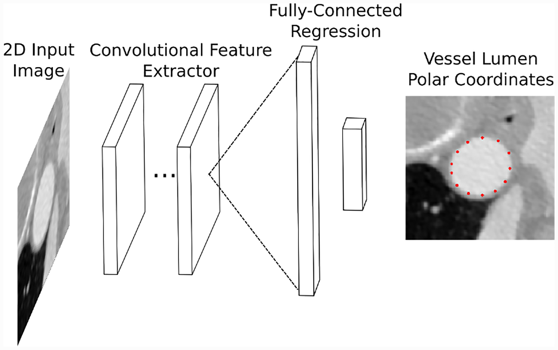
Conceptual illustration of our vessel regression neural network architecture. Convolutional layers are used to extract image features from 2D images. The image features are transformed into vessel lumen boundary points by fully-connected layers.

Fig. 3:

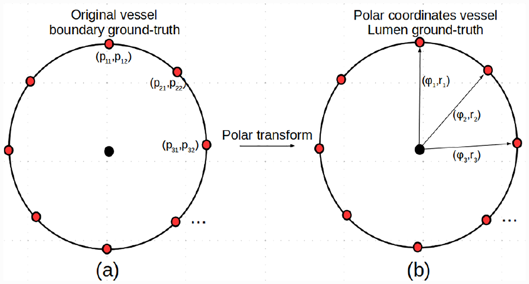
Illustration of the polar coordinates representation of a 2D cross-sectional vessel lumen boundary ground-truth label.

In mathematical terms, the CNN represents a parameterized function that transforms a 2D gray-scale image of a vessel lumen cross-section into a vector of radial distances of the vessel lumen boundary points from the centerline (Fig, 4). This is formulated as,

$$\widehat{y}=h_{\theta }(x),$$ (1)

where h_θ is the CNN function, $x\in {ℝ}^{W\times H}$ is a gray-scale 2D input image with width W and height H and $\widehat{y}\in {[0,1]}^{N_s}$ is the predicted vector of N_s radial distances of the vessel lumen boundary points from the center-line, normalized by the image dimensions. $\theta \in {ℝ}^{N_{\theta }}$ is a vector of size N_θ, containing the learnable parameters of the CNN, for which optimal values are found by optimizing the network using our training dataset.

The CNN is constructed by sequentially applying neural network layers to the input data (Fig. 4). Each layer is itself a parameterized function that acts on the output of the previous layer. Typically, each layer applies a mathematical operation, such as a linear transformation or cross-correlation, followed by an elementwise nonlinear function, known as an activation function. This process is formulated as

$$z^{(l)}=h^{(l)}\left(a^{(l-1)};{\theta }^{(l)}\right)$$ (2)

$$a^{(l)}=g^{(l)}\left(z^{(l)}\right).$$ (3)

Here l indicates the layer number, h is the layer function, z and a are the layer outputs, before and after the activation function. θ^(l) are the learnable parameters for the lth layer.

Our CNN uses a combination of fully-connected layers and convolutional layers. Fully-connected layers operate on vector inputs and apply a linear transformation defined as

$$z^{(l)}={\Theta }^{(l)}{a}^{(l-1)}+b^{(l)},$$ (4)

where Θ^(l) is a weight matrix of the layer and b^(l) is a bias term. The convolutional layers apply a cross-correlation to a three dimensional tensor input

$$z_{ijk}^{(l)}=\sum _o\sum _p\sum _q{\Theta }_{\mathit{\text{opqk}}}^{(l)}{a}_{i+o,j+p,q}^{(l-1)}+b^{(l)},$$ (5)

where Θ^(l) is a four dimensional tensor of learnable parameters. When the output of a convolutional layer is used as the input for a fully-connected layer, it is unrolled into a one dimensional vector to ensure compatibility.

The activation functions, g^(l), of each layer are necessary to allow the neural network to learn complex nonlinear relationships in the data. The activation function of the output layer of the network determines the types of outputs it can produce. Because our output is a vector with elements in the range [0, 1] we therefore use the elementwise sigmoid activation function

$$g^{(l)}(z)=\frac{1}{1+e^{-z}}.$$ (6)

For the intermediate layers we use the Leaky Rectified Linear Unit (Leaky-RELU) because it performs well when optimizing the network weights using gradient-descent

$$g^{(l)}(z)=\{\begin{array}{l}z,z>0\hfill \\ \alpha z,z\le 0.\hfill \end{array}$$ (7)

In theory, any neural network with sufficiently many parameters can learn any function [15]. However, in practice, the details of the network architecture can significantly influence its performance. While fully-convolutional networks have been extensively studied for medical image pixel classification tasks [29,34], no commonly used architectures exist for regression tasks. We therefore developed our own baseline networks and refer to them with the label ConvNet. Our ConvNet networks consist of a sequence of convolutional layers followed by a sequence of fully-connected layers (Fig. 4). The final fully-connected layer produces an output with the same size as the number of vessel lumen boundary points to be predicted. This allows us to investigate the influence of the network depth and fully-connected layer sizes.

We also investigated the GoogleNet architecture [40] due to its demonstrated performance on image classification tasks. However it was necessary to modify the GoogleNet architecture from its original image classification task to our vessel lumen boundary regression task. This is done by changing the output activation function to a linear function and resizing its final fully-connected layer to the same size as the number of vessel lumen boundary points to be predicted.

2.2. Vessel Lumen Polar Coordinates Representation

Our neural networks use a polar coordinate output representation to predict a vector of radial distances of the vessel lumen boundary points from the centerline at a specified number of angular increments (Fig. 3).

We extract local 2D lumen boundaries in the plane perpendicular to the pathline at locations where annotators segmented the vessel lumen boundary. The boundary points are represented as a matrix $p\in {ℝ}^{N_p\times 2}$ where p_i1 and p_i2 are the x and y coordinates of the ith lumen boundary point, respectively.

To normalize the extracted vessel lumen boundary we first assume the origin of p is the point (0, 0), i.e. the center of the image. We then divide the range [0, 2π] into N_s intervals, producing the vector $\varphi =\left[{\varphi }_1,\dots ,{\varphi }_{N_s}\right]$. We compute N_s radii, r(ϕ_i; p), by computing the radius of p from the origin at angles ϕ_i. The ground-truth vector of normalized distances is

$$y=\frac{1}{W/2}\left[\begin{array}{c}r\left({\varphi }_1;p\right)\\ ⋮\\ r\left({\varphi }_{N_s};p\right)\end{array}\right].$$ (8)

The output of the network, $\widehat{y}\in {[0,1]}^{N_s}$, is a vector of size N_s, with values between 0 and 1. The components of $\widehat{y}$ represent normalized distances of the vessel lumen boundary points for the chosen angles from the center of the image. The normalized distances are converted back to local 2D coordinates using

$$\left(p_{i1},p_{i2}\right)=\left(\frac{{\widehat{y}}_{i}W}{2}\text{cos}{\varphi }_i,\frac{{\widehat{y}}_{i}W}{2}\text{sin}{\varphi }_i\right).$$ (9)

Once the network is trained, for a given vessel pathline location, we compute the vessel lumen boundary at that point by extracting the local 2D cross-sectional image slice, feeding it through the trained network, transforming the network output back to local 2D coordinates and then reorienting the local 2D vessel lumen points into 3D space using the pathline information (Fig. 2).

We note that the polar coordinate axes are held constant such that the training labels and network predictions are consistent across images, e.g. the first element of y and $\widehat{y}$ always refers to the 0 radian point on the vessel lumen.

2.3. Neural Network Training Process

During training, the network’s weights are initialized according to the variance-scaling approach in [12]. The weights are optimized using a stochastic gradient-descent algorithm to minimize the selected loss function over the 2D image and ground-truth vessel lumen pairs from our training dataset. We describe the training data collection process for a single labeled image volume, as it is straightforward to extend to multiple images.

Let X denote a gray-scale medical image volume with N_x, N_y, N_z voxels in the height, width and depth directions, respectively. Associated with the image X is a set of vessel pathlines. Each pathline is represented as a set of N_p points, $P=\left\{v_1,\dots ,v_{N_p}\right\}$, with each $v_i\in {ℝ}^3$ indicating a 3D coordinate in physical space along the pathlines.

At specific locations along the pathline, expert annotators have segmented the vessel lumen boundary. Each lumen boundary is also represented as a set of 3D physical coordinates. The 3D lumen boundary is projected onto the local 2D plane, perpendicular to the pathline at that location. We define $p_j^P$ to be the jth ground-truth lumen boundary point set associated with the pathline P.

The vessel lumen boundaries represent the ground-truth output data for our training process. The input data are 2D cross-sectional images of the vessel at the pathline locations where a lumen boundary was segmented. The input images, x_i, are extracted by interpolating the pixel values of X in the plane perpendicular to the pathline at each lumen location (Fig 2b).

Extracting lumen boundary points and cross-sectional image slices for each lumen location for each pathline then produces our training dataset of input image and ground-truth lumen pairs. We apply the angular distance transform to each ground-truth lumen boundary $p_i^P$ to transform it to a ground-truth vector y_i that can be used to train the neural network. As such, our dataset becomes a set of pairs

$$D=\left\{\left(x_1,y_1\right),\dots ,\left(x_{N_d},y_{N_d}\right)\right\}.$$ (10)

To finalize the neural network training procedure, we define a loss function and use a stochastic gradient-descent algorithm to find values for the network weights that approximately minimize the loss function over the training data. For the loss function we use the square error

$$l(y,\widehat{y})=\sum _i{\left(y_i-{\widehat{y}}_i\right)}^2,$$ (11)

where y_i and ${\widehat{y}}_i$ represent the ith ground-truth normalized lumen and neural network prediction respectively. While other loss functions could be used, such as the absolute error, the square error was found to be sufficient for our purposes and thus investigation of additional loss functions is left as an area of future research. The expected loss for a given set of training examples is then

$$L(X,Y;\theta )=\frac{1}{N_b}\sum _{i=1}^{N_b}l\left(y_i,h_{\theta }\left(x_i\right)\right),$$ (12)

where X and Y are sets containing a select of input images and corresponding normalized ground-truth vessel lumen boundary vectors. We then optimize the weights of our CNN using the stochastic gradient-descent ADAM algorithm due to its accelerated convergence properties [19].

We note that the described training data format was used as it is the standard format used in SimVascular. Our proposed network treats input images independently, thus it is not a hard requirement to train on cross-section slices from whole vessels or models. However, the training dataset should contain cross-section images and vessel lumen examples that are representative of those that will be encountered during typical cardiovascular model construction.

2.4. Dataset

Our dataset consists of 50 CT and 54 MR contrast-enhanced 3D medical image volumes, all publicly available from the Vascular Model Repository (VMR)² [47]. For each of the image volumes, the VMR also contains vessel pathlines, segmentations, 3D patient-specific models and hemodynamic simulation results (shown in Fig. 1 for a single case). Each model typically has multiple vessel pathlines, each of which are segmented at numerous locations along the path. All segmentations contained in the VMR were created in SimVascular by users with expert anatomical knowledge. The image volumes in the VMR have anisotropic voxel spacing, therefore we resampled all volumes to an isotropic voxel spacing of 0.029cm. This voxel spacing was chosen as it ensures the largest vessel diameter to be around 100 pixels. This in turn allows a relatively small window size to be used for the neural network which reduces computation and memory requirements. We split the data into training, validation and testing sets, of 76, 4 and 14 volumes, respectively.

Local 2D vessel cross-section images and corresponding lumen points were extracted (as described in Section 2.3). We used a window size of 160 × 160 pixels to allow the full range of vessel sizes to be represented with sufficient resolution. This resulted in 16004, 239 and 6317 cross-section images and vessel lumen boundary point labels for the training, validation and testing sets respectively.

2.5. Preprocessing and Data Agumentation

For our particular use-case, the CNN operates on the 2D cross-sectional images extracted along the vessel pathlines. Given a gray-scale image $x\in {ℝ}^{H\times W}$, we first compute a normalized image $\tilde{x}$ by normalizing x to have zero mean and unit variance pixel values, so that

$$\tilde{x}=\frac{x-{\mu }_x}{{\sigma }_x},$$ (13)

where μ_x and σ_x are the mean and standard deviation of the pixel values of x and are given by

$${\mu }_x=\frac{1}{HW}\sum _{i=1}^H\sum _{j=1}^W{x}_{ij},$$ (14)

and

$${\sigma }_x={\left(\frac{1}{HW}\sum _{i=1}^H\sum _{j=1}^W{\left(x_{ij}-{\mu }_x\right)}^2\right)}^{1/2}.$$ (15)

During training we further augment the dataset, on the fly, by randomly rotating images between 0 – 2π radians and applying random translation perturbations to each training image and vessel lumen boundary pair. The maximum translation distance is determined individually for each vessel lumen as a fraction of the idealized lumen radius. The translation distance was chosen this way to emulate human vessel pathline placement error, where for larger vessels there is more room to place a pathline point, leading to larger absolute variation as compared to smaller vessels.

3. Experiments

For our experimentation we compare the predicted lumen boundaries of our trained networks, and three reference fully-convolutional pixel classification networks, against the ground-truth lumen boundaries in our dataset. For the comparison we use several common segmentation accuracy metrics.

We also measure the average accuracy between expert SimVascular users on an MR cerebrovascular, pulmonary, coronary vasculature and CT aortic aneurysm case to indicate human accuracy and segmentation uncertainty. We then compare the segmentations generated by GoogleNet-c30, the best performing network, on the same cases.

Finally we calculate the amount of manual segmentation effort that would be saved by using the network to compute lumen segmentations in practice.

3.1. Performance Metrics

We compared the produced segmentations using several commonly applied metrics [41].

The first metric is the DICE metric which measures the similarity between two sets. Letting A and B denote the sets of points contained on the boundary and in the interior of each segmentation, the DICE is given by:

$$\text{DICE}(A,B)=\frac{2|A\cap B|}{\left|A\right|+\left|B\right|}.$$ (16)

The second metric is the Hausdorff Distance (HD) which has a lower bound of 0 (perfect match) with no upper bound. Letting A and B be the sets of points contained on the boundaries of the two segmentations, the HD measures the maximum minimum distance between all points in the sets and is given by:

$$d_H(A,B)=\text{max}\left\{\underset{a\in A}{\text{sup}}\underset{b\in B}{\text{inf}}d(a,b),\underset{b\in B}{\text{sup}}\underset{a\in B}{\text{inf}}d(a,b)\right\},$$ (17)

where d(a, b) is a distance function, for which we use the euclidean norm d(a, b) = ||a − b||_2.

The final metrics is the Average Symmetric Surface Distance (ASSD) which computes the average minimal distance between the surface points of two sets A and B. Let $\tilde{A}$ and $\tilde{B}$ be sets of the surface points in A and B, respectively. The ASSD is then:

$$\text{ASSD}(A,B)=\frac{1}{\left|\tilde{A}\right|+\left|\tilde{B}\right|}\left(\sum _{a\in \tilde{A}}\underset{b\in \tilde{B}}{\text{min}}d(a,b)+\sum _{b\in \tilde{B}}\underset{a\in \tilde{A}}{\text{min}}d(b,a)\right),$$ (18)

where d is again the Euclidean norm.

3.2. Network Architectures and Hyperparameters

We trained all networks using the ADAM [19] stochastic gradient algorithm, for 300,000 training image batches with a batch size of 4. For the baseline networks the learning rate started at 1·10⁻³. For the GoogleNet networks a starting learning rate of 5·10⁻⁵ was required to obtain convergence. For all networks the learning rate was decreased by a factor of 3 after the first 2000 batches, then by a factor of 10 after 5,000, 10,000 and 15,000 batches, respectively. We further investigated the use of 15, 30 and 45 angular increments for the vessel lumen boundary. Input images were cropped to dimensions of 160 × 160 and used a fixed resolution of 0.029cm/pixel allowing both large and small vessel to fit inside the input window size. During training, images and ground-truth lumen were randomly rotated between 0 – 2π radians and randomly translated a distance of up to 65% of the ground-truth vessel radius.

The ConvNet networks and GoogleNet networks we considered, and the labels we use to refer to them, are described in Tables 1 and 2 respectively. All networks used the leaky-RELU activation with a coefficient value of 0.2. The ConvNet networks used 3 × 3 convolution filters with 32 channels throughout. No regularization was used other than the dropout layers that are included in the GoogleNet architecture.

Table 1:

Baseline network naming conventions.

Name	Conv. layers	FC layers	FC layer sizes
ConvNet-1	10	2	250, 15
ConvNet-2	20	2	250, 15
ConvNet-3	10	3	1000, 250, 15
ConvNet-4	20	3	1000, 250, 15

Table 2:

GoogleNet naming conventions.

Name	Architecture	Output dimension
GoogleNet	GoogleNet	15
GoogleNet-c30	GoogleNet	30
GoogleNet-c45	GoogleNet	45

The performance of the ConvNet and GoogleNet networks was compared to the architectures used in our previous work [27]: the commonly used UNet [34], DeepLab-ASPP [5] and CENet [11] image segmentation networks. These networks were retrained for 2D vessel segmentation, using our training data. During testing, the marching-squares algorithm was used to extract the vessel lumen boundary from the segmentations produced by the image segmentation networks.

3.3. Segmentation Uncertainty Measurements

To measure the uncertainty in our ground-truth segmentation data, we selected four image data sets from the VMR, designated as

• Cerebro: MR image of the cerebrovascular region of a patient with a left anterior cerebral aneurysm.

• AAA: A CT scan of abdominal region of a patient with an abdominal aortic aneurysm.

• KDR: MR image of coronary arteries and Aorta of a patient with Kawasaki Disease.

• Pulmonary: MR image of the pulmonary vasculature.

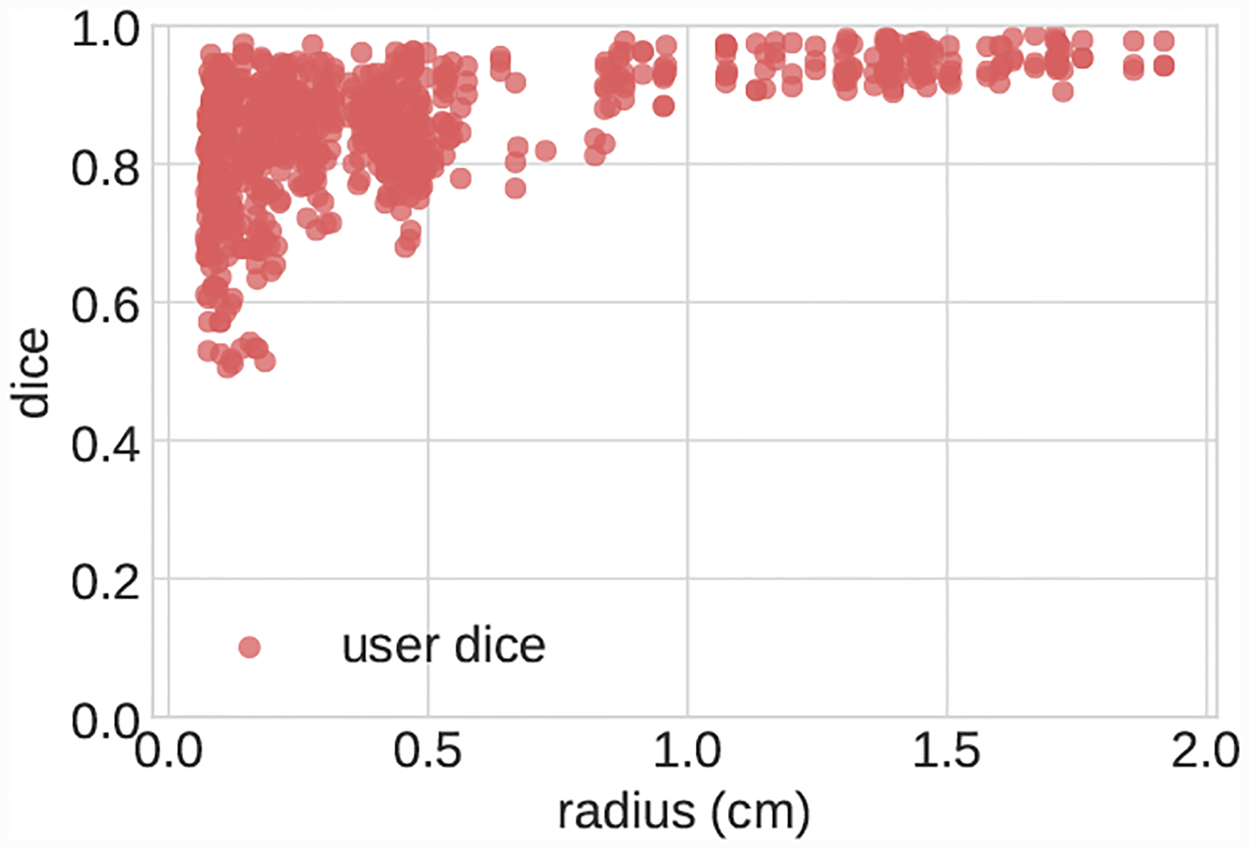
Models for each case are shown in Fig. 21. For each image, several vessel pathlines, created by anatomical experts, were selected from the VMR, where pathlines were selected to provide sufficiently large samples of both small and large vessels. For each case, three expert SimVascular users where tasked with creating 2D vessel segmentations at points along the vessel pathlines. For AAA and Pulmonary, segmented pathline locations from the VMR were used. For Cerebro and KDR, segmentations were created every 5 path points. In total this resulted in 290 segmentations per expert, enabling 870 pairwise DICE measurements.

Fig. 21:

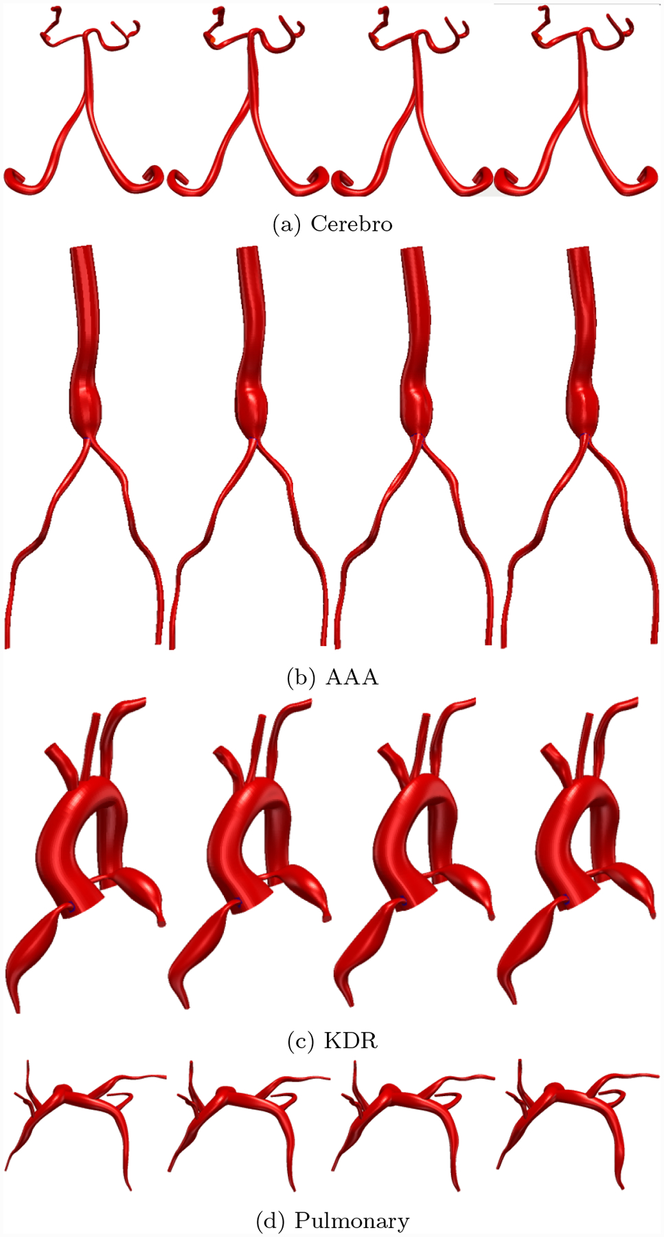
Comparison between 3D Cardiovascular models produced by neural network segmentations and SimVascular experts. First column is GoogleNet-c30, subsequent columns are the experts.

Exact sample sizes for each case and a number of vessel radii are reported in Table 6. We then compared the pairwise DICE accuracy between each of the three experts as well as the segmentations generated by GoogleNet-C30 at similar locations for all cases. That is to say, expert 1 was compared to expert 2, expert 2 to expert 3 and expert 3 to expert 1, in addition to comparing GoogleNet-c30 to each individual expert.

Table 6:

User Test sample sizes. Radius in number of pixels (_pix) in minimum native image resolution.

image	0pix < r ≤ 5pix	5pix < r ≤ 10pix	10pix < r ≤ 20pix	20pix < r ≤ 60pix
Cerebro	186	51	0	0
AAA	0	170	3	111
KDR	3	36	95	50
Pulmonary	104	39	23	0

The DICE statistics are then binned by segmentation radius in number of pixels in the minimum native resolution of each image across coronal, sagittal and axial directions.

4. Results

4.1. Overall Network Performance

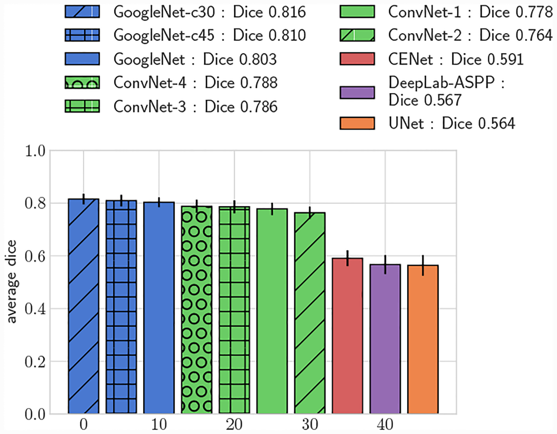
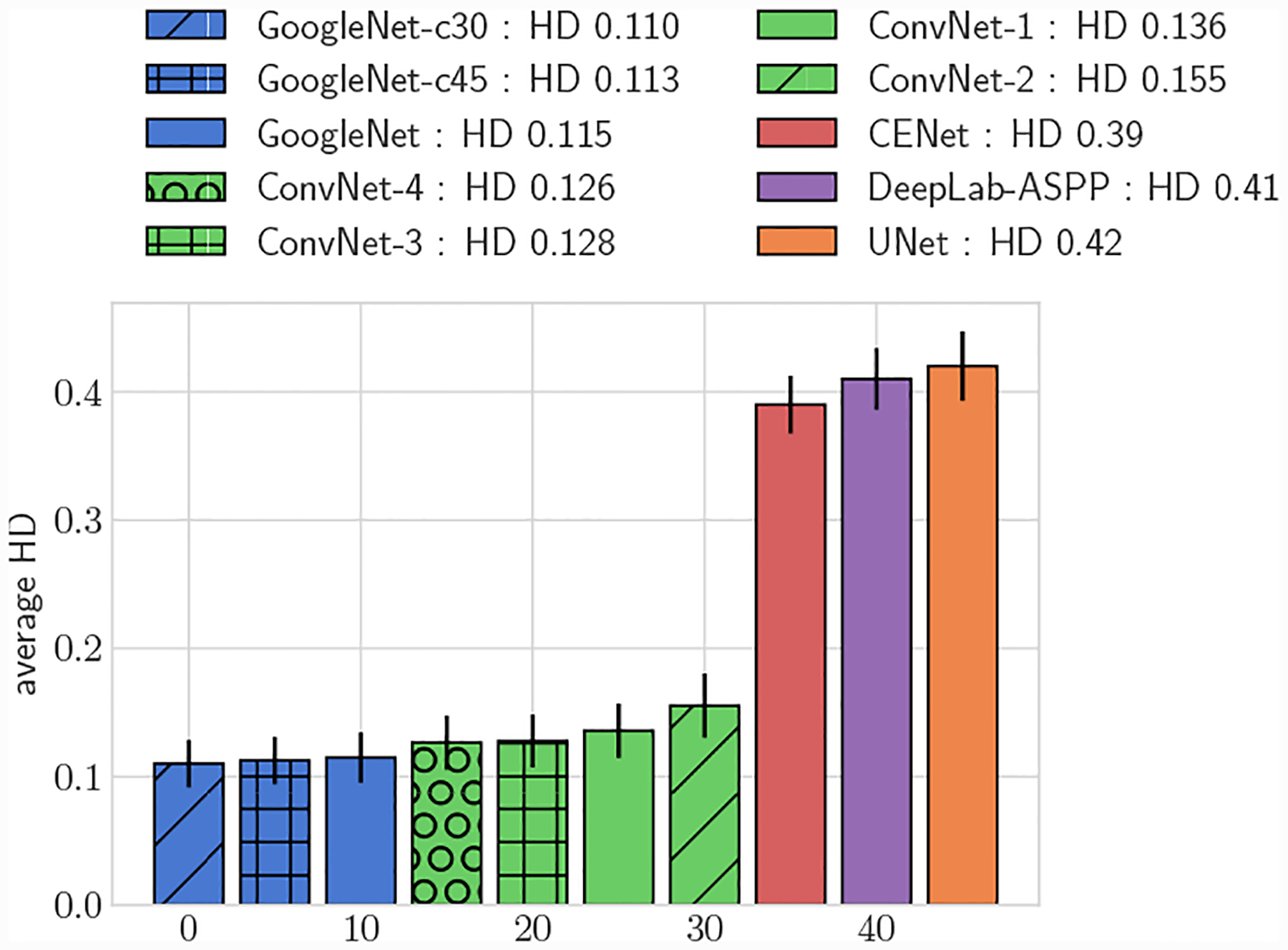
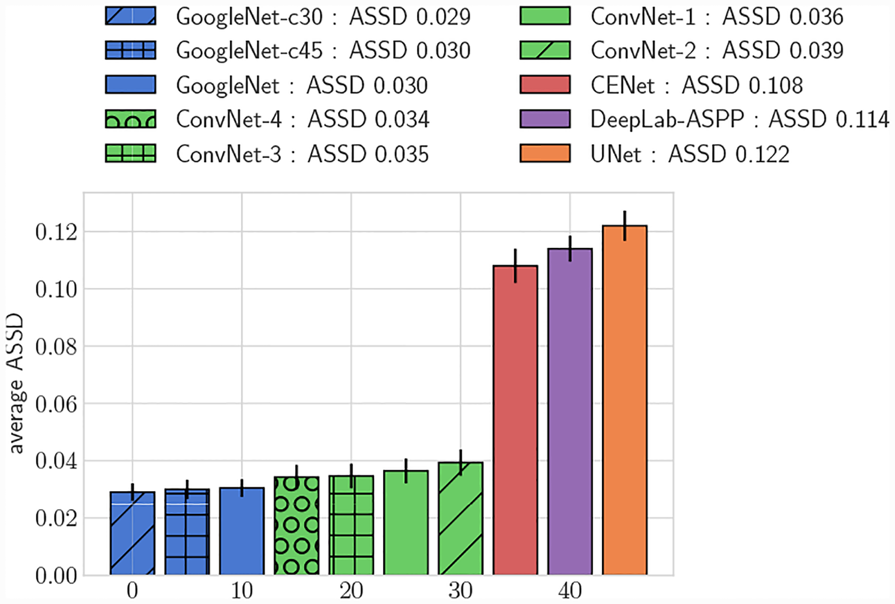
In addition to reporting results on the full test set, we also divided the test set into large vessels (radius > 0.4cm) and small vessels (radius < 0.4cm) and reported results on these subsets. We analyzed DICE accuracy on both 2D segmentations (Figs. 5–7) and over whole 3D vessel models (Figs. 8–10). For the 3D vessel models we further investigated HD and ASSD metrics (Figs. 11,12). The choice of cutoff radius was based on our human segmentation uncertainty findings, in which uncertainty was relatively larger for vessels with a radius smaller than 0.4cm (Figs. 15, 16). While the user ASSD is smaller for smaller vessels than for larger vessels, when computed as a fraction of the vessel radius it is still proportionally larger for smaller vessels. All p-values are computed using one-, or two-sided t-tests, where appropriate, for paired samples. When comparing results between experiments the means are balanced with similar weights for small and large vessels.

Fig. 5:

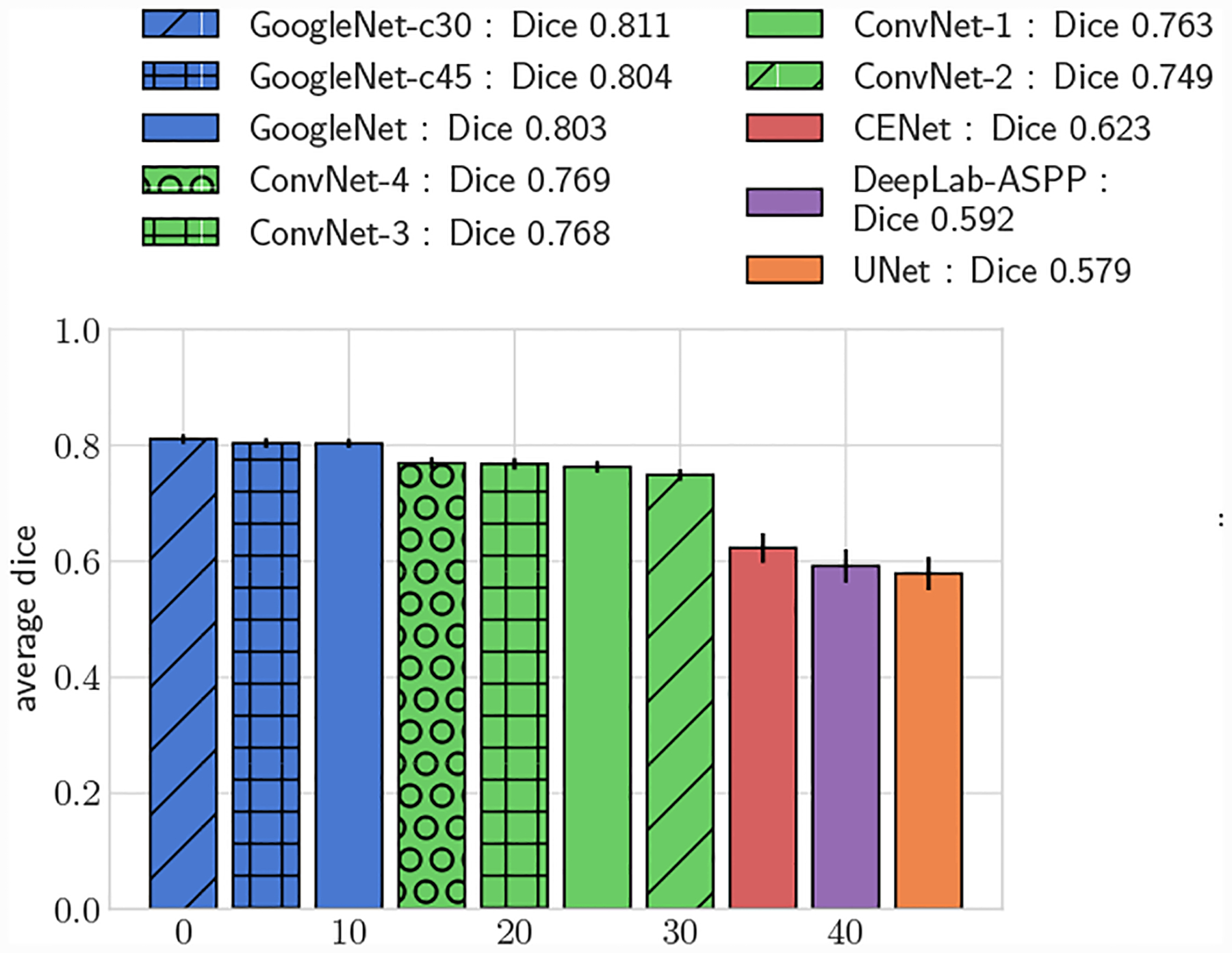
Average DICE, full test set.

Fig. 7:

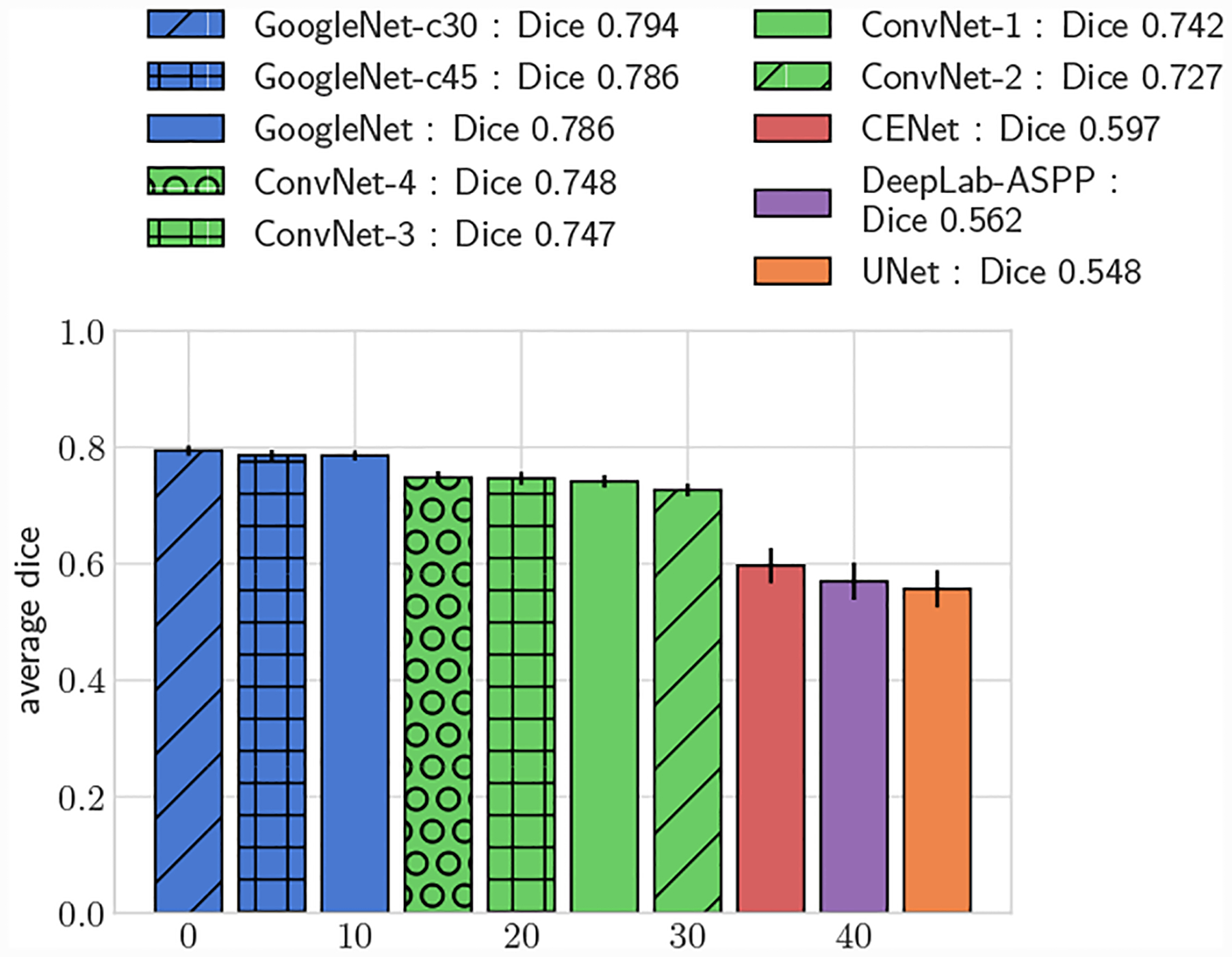
Average DICE for test set, small vessels (r ≤ 0.4cm)

Fig. 8:

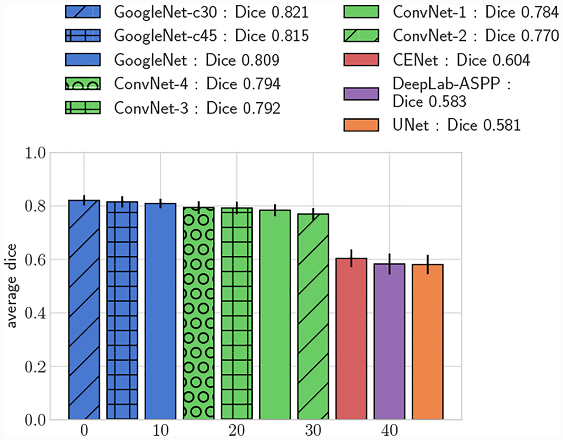
Average 3D DICE, full test set.

Fig. 10:

Average 3D DICE for test set, small vessels (r ≤ 0.4cm)

Fig. 11:

Average 3D HD, full test set

Fig. 12:

Average 3D ASSD, full test set

Fig. 15:

Scatterplot of pairwise DICE scores for segmentations produced during user uncertainty experiment.

Fig. 16:

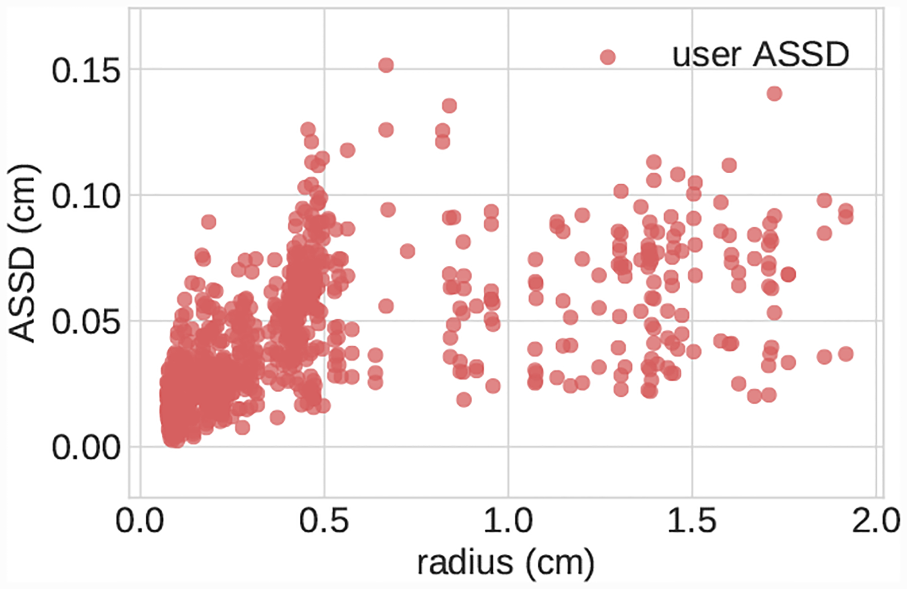
Scatterplot of pairwise ASSD scores for segmentations produced during user uncertainty experiment.

All GoogleNet networks performed significantly better than all ConvNet networks across all metrics (p < 0.05), highlighting the improvements gained from the increased depth and inception layers. For both 2D and 3D metrics, mean DICE amongst the GoogleNet networks was not significantly different for large vessels, but for small vessels GoogleNet-c30 obtained the highest mean DICE (p < 0.05). Comparing among the ConvNet networks, ConvNet-3 and ConvNet-4 outperformed ConvNet-1 and ConvNet-2 across all metrics, highlighting the need for multiple fully-connected layers to learn the nonlinear transformation from image features to vessel lumen boundary points.

Across the entire test-set, for both 2D and 3D metrics, all GoogleNet regression networks produced significantly higher average DICE scores than the UNet, DeepLab-ASPP and CENet image segmentation networks (p < 0.01) (Fig. 5). For large vessels the average dice scores of the GoogleNet networks was significantly better than the FCNN networks (Fig. 6). However, the majority of the difference can be attributed to the higher average DICE scores produced by the vessel regression networks on small vessels (p < 0.01) (Fig. 7). Similar results are reflected in the HD and ASSD scores (Fig. 11, 12).

Fig. 6:

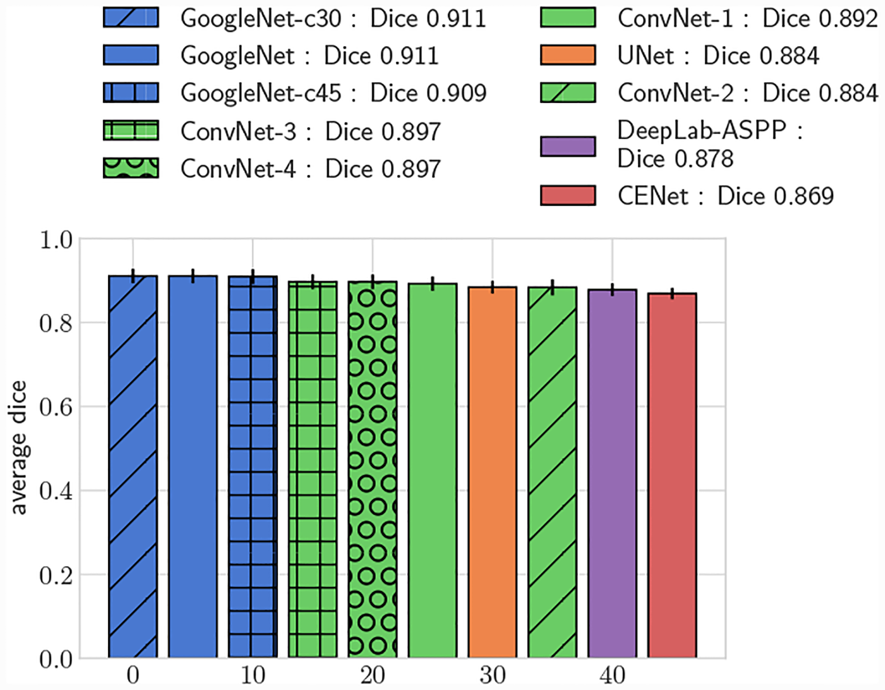
Average DICE for test set, large vessels (r > 0.4cm)

We further compared the performance improvement our methods by adapting the UNet architecture to directly predict vessel lumen through polar coordinate regression, labeled as UNet-c30. UNet-c30 had lower average DICE scores compared to all GoogleNet networks for both large and small vessel test sets (p < 0.05). However average DICE scores were larger when compared to the pixel segmentation networks (p < 0.05). This highlights that lumen prediction through polar coordinate regression leads to improved accuracy over segmentation through pixel classification even with the same network architecture.

4.2. Segmentation Uncertainty Measurements

For the largest vessels (20_pix < r ≤ 60_pix) the mean DICE score of GoogleNet was significantly higher than human experts for AAA, but not signficiantly different for KDR, indicating performance comparable to human experts.

For the second largest vessel bin (10_pix < r ≤ 20xp) for KDR mean DICE scores between human experts and GoogleNet were not significantly different. Human expert Pulmonary mean DICE scores were signficantly higher than GoogleNet.

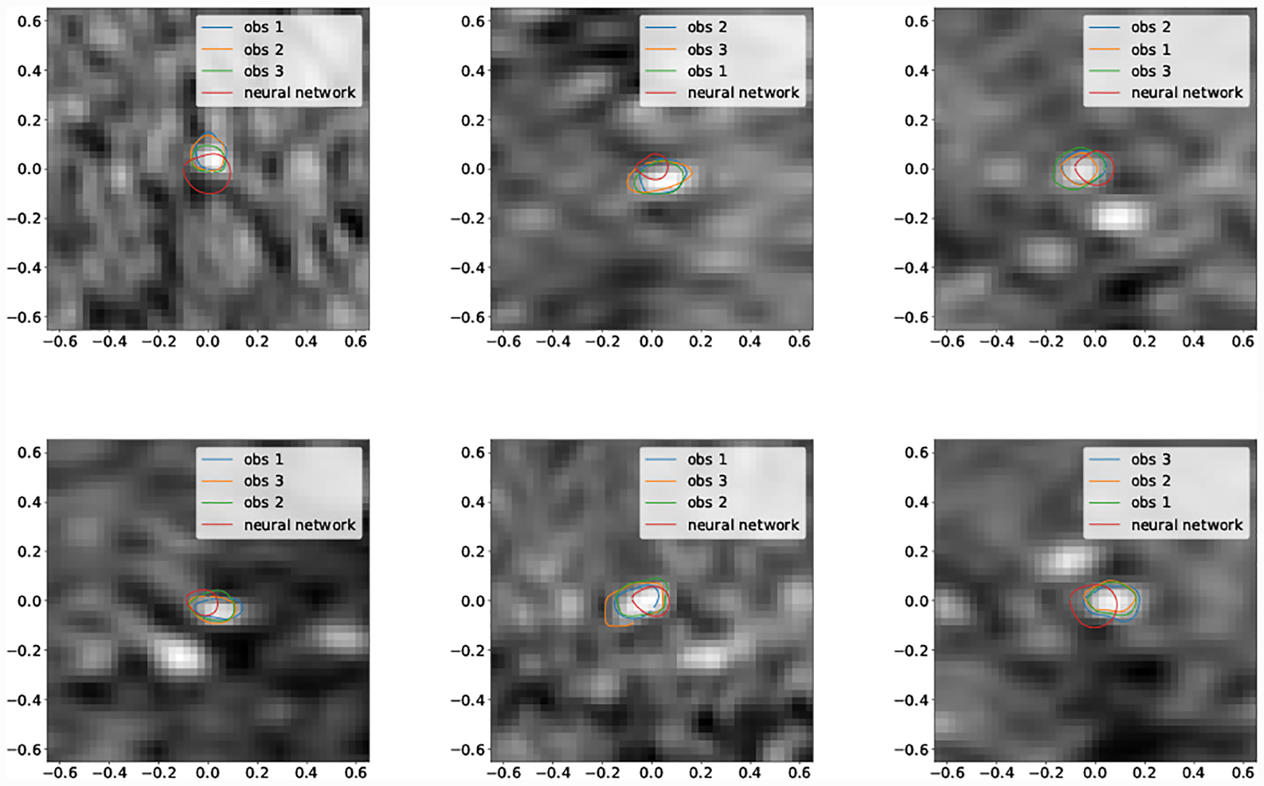
For the second smallest vessel size bin (5_pix < r ≤ 10_pix) mean DICE scores for GoogleNet and human experts was not significantly different for Cerebro and AAA. For KDR and Pulmonary human experts achieved significantly higher mean DICE scores. Examining the lowest DICE scoring segmentations produced by GoogleNet for KDR (Fig. 20) and Pulmonary (Fig. 18) shows that typically large DICE errors are due to poor resolution, unclear vessels, or surrounding tissue.

Fig. 20:

Selection of worst case DICE error segmentations for KDR (obs indicates human expert).

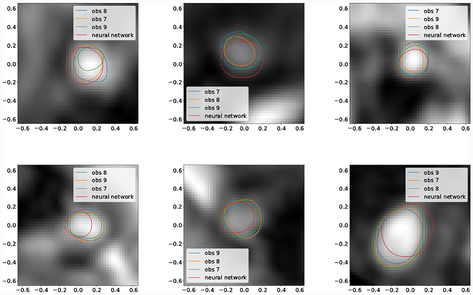
Fig. 18:

Selection of worst case DICE error segmentations for Cerebro (obs indicates human expert).

For the smallest vessel size bin, mean DICE was not signficantly different for Pulmonary, but for Cerebro human expert mean DICE was significantly higher.

Mean inter-expert DICE agreement was the same for the Cerebro and KDR models (p < 0.05) (Fig 23). For the AAA and pulmonary models there were statistically significant differences. For the pulmonary model this can be attributed to the lower resolution and image quality leading to increased expert DICE variance (Tab 4, Figs 23,19). For the AAA model differences in expert agreement were due to varying interpretations of thrombus formation in aneurysm regions in addition to regions of poor image quality. Similar trends are reflected in the median DICE scores (Tab. 5).

Fig. 23:

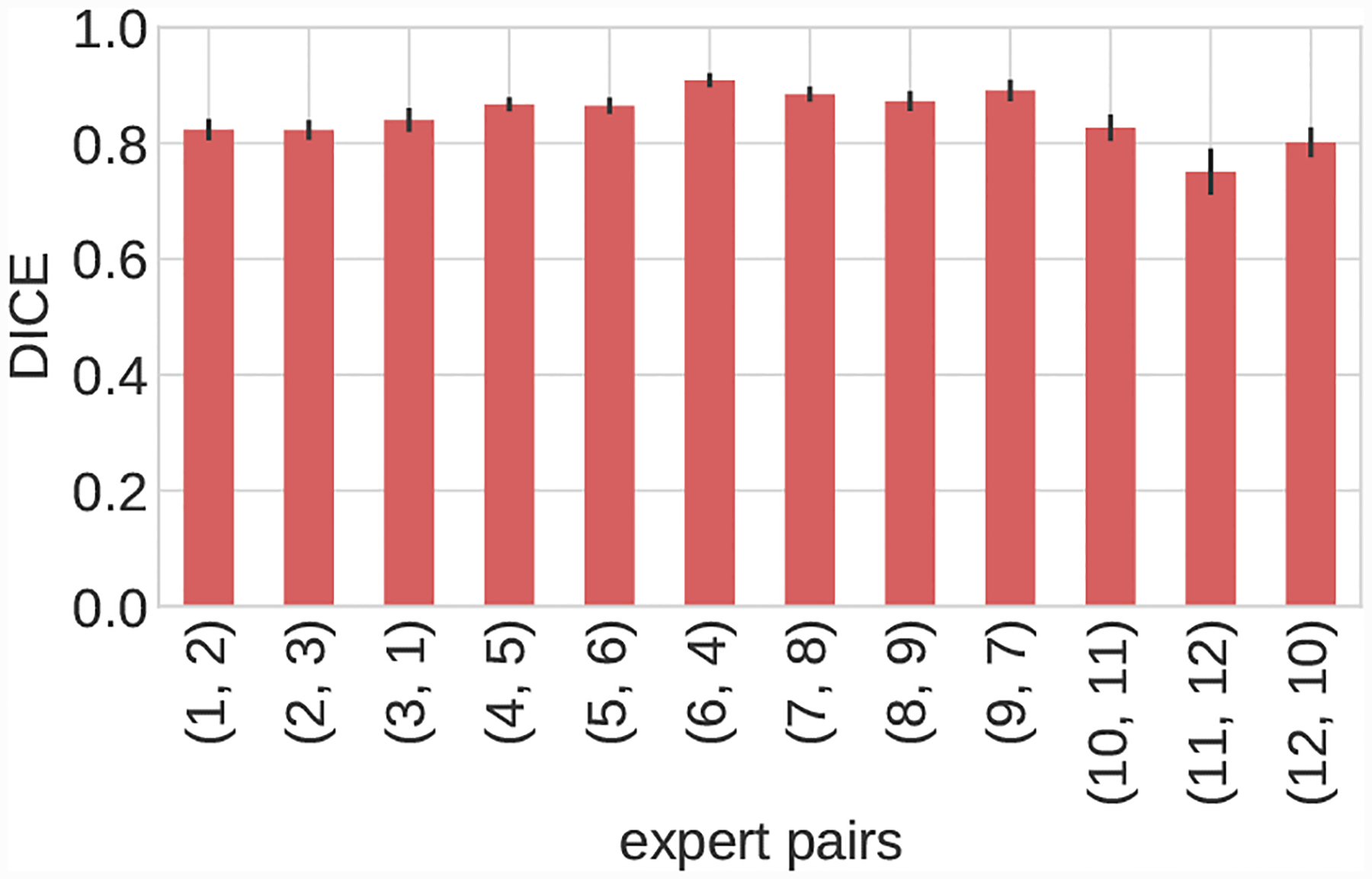
Inter-expert mean DICE agreement for each image in the user test-set. Image volumes organized as follows, 1–3: Cerebro, 4–6: AAA, 7–9: KDR, 10–12: Pulmonary.

Table 4:

User test mean DICE scores with two-sided 95% confidence interval. Radius in number of pixels (_pix) in minimum native image resolution. Samples with sample size smaller than 10 not reported.

image	method	0pix < r ≤ 5pix	5pix < r ≤ 10pix	10pix < r ≤ 20pix	20pix < r ≤ 60pix
Cerebro	human	0.813 ± 0.013	0.885 ± 0.011	*	*
Cerebro	GoogleNet-c30	0.680 ± 0.019	0.861 ± 0.017	*	*
AAA	human	*	0.837 ± 0.007	*	0.946 ± 0.004
AAA	GoogleNet-c30	*	0.881 ± 0.007	*	0.958 ± 0.004
KDR	human	*	0.860 ± 0.020	0.863 ± 0.013	0.936 ± 0.011
KDR	GoogleNet-c30	*	0.789 ± 0.032	0.874 ± 0.013	0.934 ± 0.022
Pulmonary	human	0.748 ± 0.022	0.870 ± 0.017	0.883 ± 0.023	*
Pulmonary	GoogleNet-c30	0.726 ± 0.020	0.762 ± 0.045	0.810 ± 0.036	*

Fig. 19:

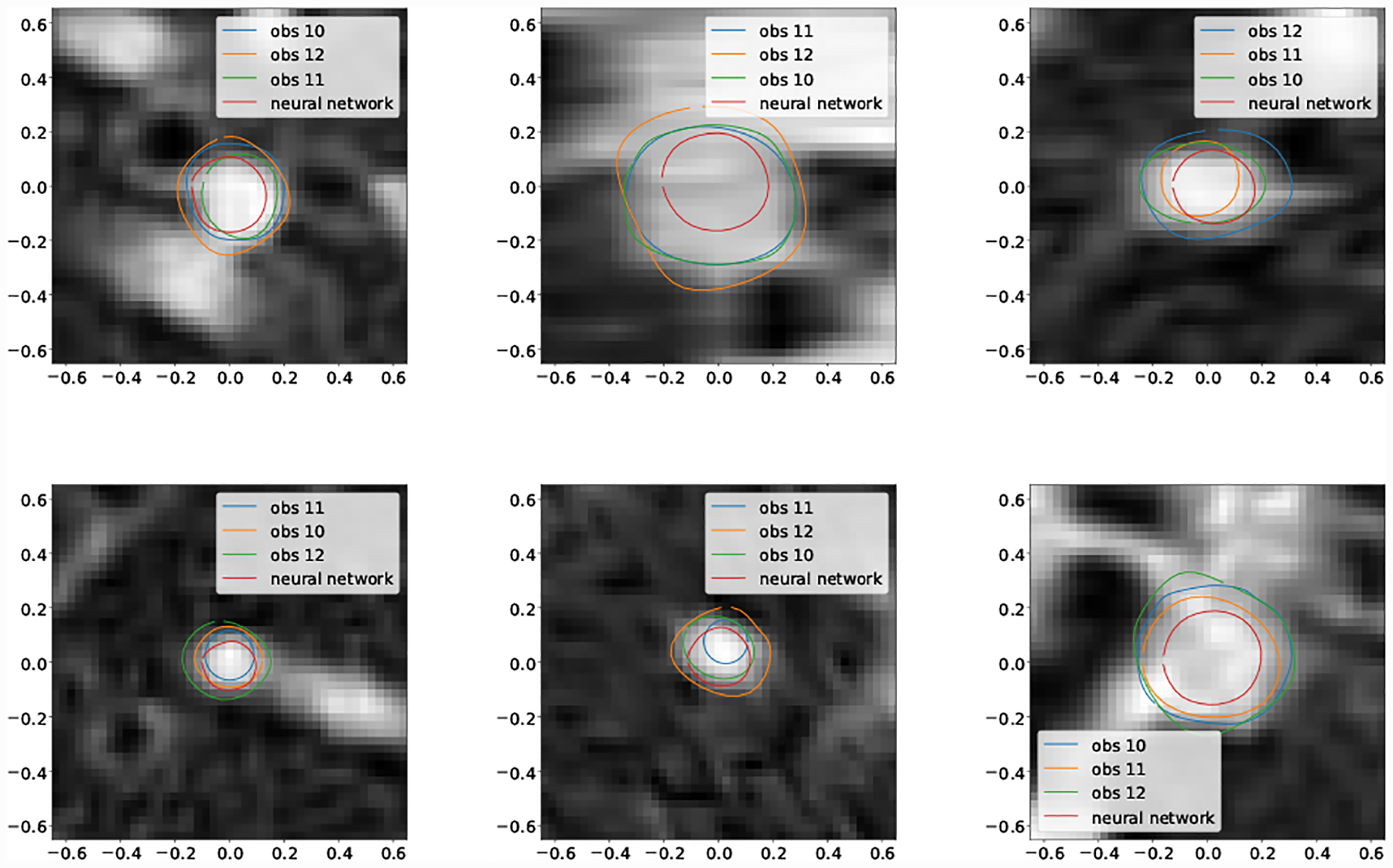
Selection of worst case DICE error segmentations for pulmonary (obs indicates human expert).

Table 5:

User test median DICE scores. Radius in number of pixels in minimum native image resolution. Samples with sample size smaller than 10 not reported.

image	method	0pix < r ≤ 5pix	5pix < r ≤ 10pix	10pix < r ≤ 20pix	20pix < r ≤ 60pix
Cerebro	human	0.821	0.883	*	*
Cerebro	GoogleNet-c30	0.697	0.869	*	*
AAA	human	*	0.838	*	0.943
AAA	GoogleNet-c30	*	0.887	*	0.964
KDR	human	*	0.876	0.869	0.945
KDR	GoogleNet-c30	*	0.807	0.881	0.948
Pulmonary	human	0.760	0.873	0.904	*
Pulmonary	GoogleNet-c30	0.735	0.779	0.813	*

Examining the smallest vessels for Cerebro (Fig. 18) demonstrates that the pathline is often outside the vessel, leading GoogleNet to produce inaccurate segmentations.

Examining the selection of best case DICE score segmentations (Fig. 17) it is clear that network segmentation accuracy is best when the vessel has clear borders and sufficient resolution. Our findings agree with user experience, and are in line with decreasing resolution relative to vessel size when proceeding distally in the vascular tree.

Fig. 17:

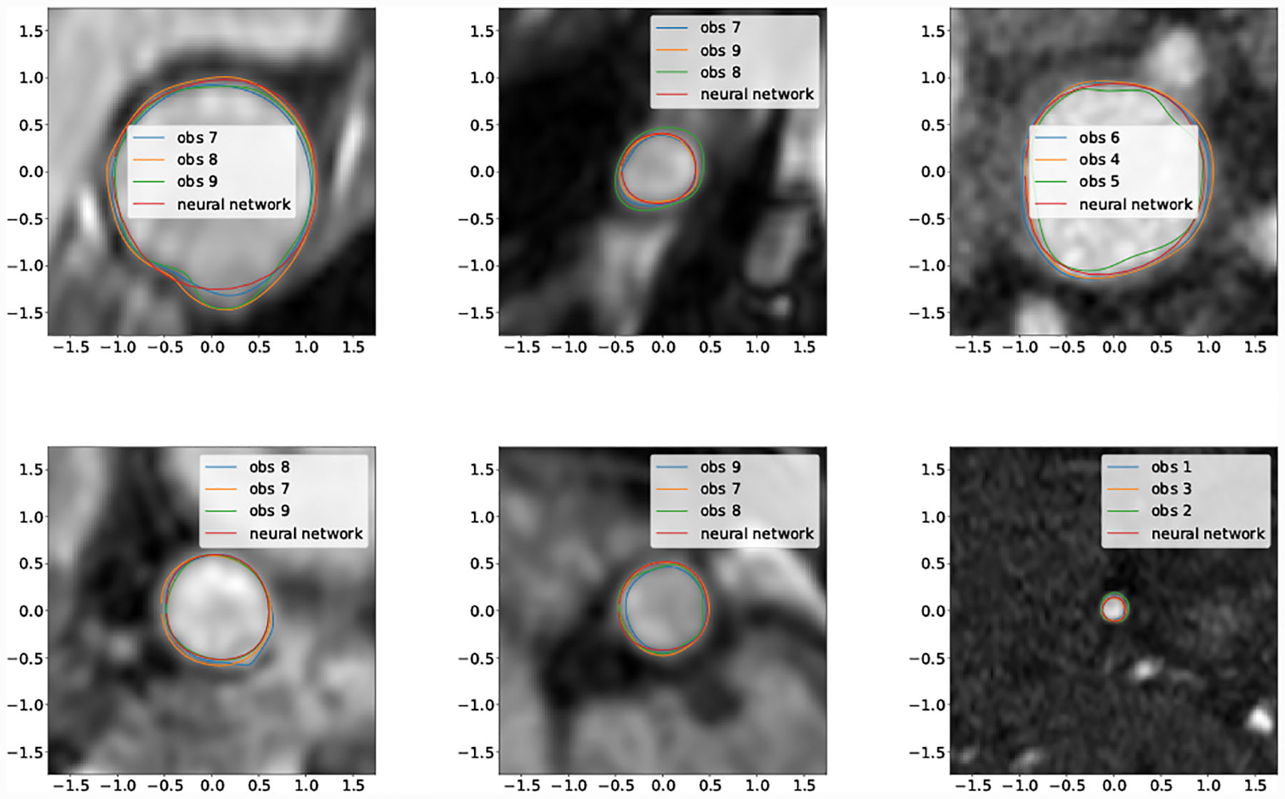
Selection of best case DICE segmentations for all images (obs indicates human expert).

3D cardiovascular models produced using the GoogleNet-c30 network were qualitatively similar to those produced by the human experts (Fig. 21). In particular, Important model features such as aneurysm shape in the KDR and AAA models were well captured. Example performance in difficult segmentation locations, containing e.g. thrombus, calcification and branching vessels is also shown (Fig. 22).

Fig. 22:

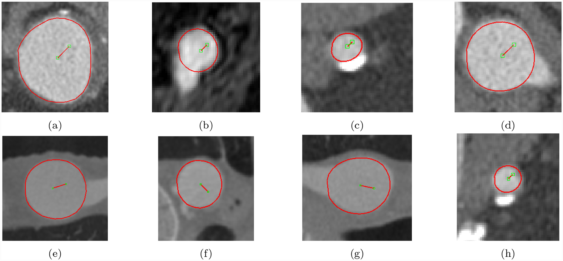
Example GoogleNet-c30 predicted lumen for hard cases containing aneurysm thrombus, calcification and branching vessels. Images were taken from image volumes in the user-test set.

4.3. Runtime Performance, Memory Usage and Segmentation Time Savings

Computing 100 segmentations, without use of a GPU, with GoogleNet-c30 took on average 3.62 seconds on a laptop with a 2.4Ghz i7 CPU. The average time to compute a single segmentation is therefore on the order of 0.036 seconds. The total RAM used to load the network was 57.7 megabytes.

Subjects from our segmentation uncertainty experiment reported that manual segmentation took on average, an order of 5–10 seconds for a single segmentation. Therefore our proposed CNN segmentation method is significantly faster than manual segmentation when compared on single segmentations, even when using conventional CPUs and commodity hardware.

Under the assumption that a human expert would accept a generated segmentation, provided it scored above average DICE as measured compared to human expert DICE accuracy, we can obtain an estimate for the percentage in segmentation time savings provided by use of vessel lumen regression (Tab 7). Time savings range from 15% to as high as 80% depending on vessel size and anatomical region. For AAA and KDR in the ranges (10 < r ≤ 20) and (20 < r ≤ 60) time savings were 65 – 70%. However for Pulmonary the percentage time savings was 26.09%, which corresponds with the poorer resolution observed for many of the vessels for this case. For the two smallest vessel bins, AAA GoogleNet DICE was above average compared to human experts 80% of the time, corresponding to the clearer vessels and good resolution for this case. For KDR, in the range 5 < r ≤ 10, the percentage of GoogleNet segmentations above human agreement was 30.56%, but for larger bins the time savings approximately doubled. This is in correspondence with the fact that, while not unreasonable, the segmentations produced by GoogleNet in the presence of surrounding tissue and poor vessel resolution deviate substantially from those of human experts (Fig. 20).

Table 7:

Percentage of segmentations generated by GoogleNet-c30 with above average DICE as compared to human experts. Indicates percentage segmentation time savings. Samples with sample size smaller than 10 not reported.

image	0pix < r ≤ 5pix	5pix < r ≤ 10pix	10pix < r ≤ 20pix	20pix < r ≤ 60pix
Cerebro	15.59%	37.25%	*	*
AAA	*	80.00%	*	70.27%
KDR	*	30.56%	65.26%	72.00%
Pulmonary	40.38%	25.64%	26.09%	*

5. Open-Source Release

We have made the CNN-based segmentation pipeline in this work freely and publicly available via the open-source SimVascular project. The code is implemented in Python with the Tensorflow library and C++ to expose the user-interface. The code does not require specialized hardware such as GPUs, making it accessible to users with commodity hardware. Pre-trained binaries for the best performing network (GoogleNet-C30) are distributed, allowing the pipeline to be used by the modeling community without the need to train networks.

6. Conclusions

Our results show that CNNs using a vessel lumen regression formulation and a neural network architecture with sufficient learning capacity can achieve similar accuracy to human experts manually segmenting vessel lumens for a variety of anatomical regions and multiple imaging modalities. However, obtaining high DICE segmentations from the network, as measured compared to human experts, is conditional on sufficient image resolution, vessel visibility and vessel center accuracy. In particular for small vessels, vessel center accuracy can be problematic and suggests that vessel lumen regression could be improved through additional vessel localization steps.

For large vessels segmentation time savings of roughly 65 – 70% were observed as 65 – 70% of the segmentations produced by our CNN pipeline were of similar or higher accuracy to the average agreement between expert SimVascular users. For small vessels the time savings range from 15 – 40% for cases with poor image resolution and vessel pathline noise, but was 80% for cases with better imaging conditions. For realistic models with hundreds of vessels to be segmented, on non-specialized hardware, our pipeline results in time savings of multiple hours of segmentation effort. Our CNN segmentation pipeline thus significantly reduces the turnaround time to perform cardiovascular patient-specific simulations, paving the way for their use in clinically realistic settings and making simulation studies on large patient cohorts more accessible.

While our neural network based lumen regression pipeline significantly accelerates 2D cardiovascular segmentation, the vessel centerline detection step still needs to be performed manually. The automation of vessel centerline detection is an area for future work. Automated centerline detection could be combined with our lumen regression pipeline to further accelerate the entire cardiovascular model building workflow.

Fig. 9:

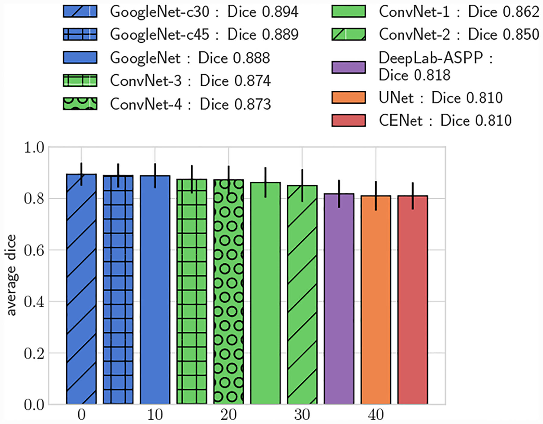
Average 3D DICE for test set, large vessels (r > 0.4cm)

Fig. 13:

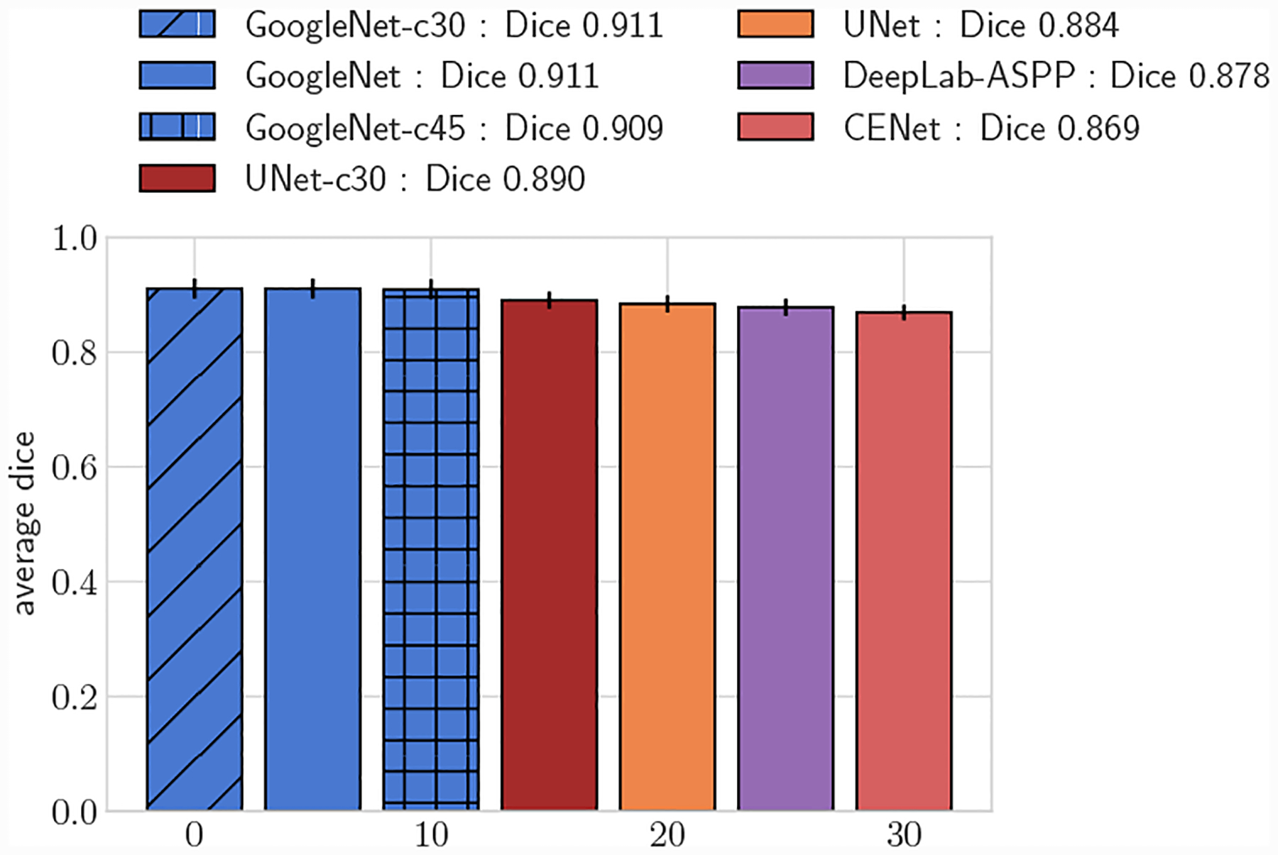
Comparison of UNet lumen regression network to GoogleNet-c30 and segmentation networks. Average DICE for test set, large vessels (r > 0.4cm)

Fig. 14:

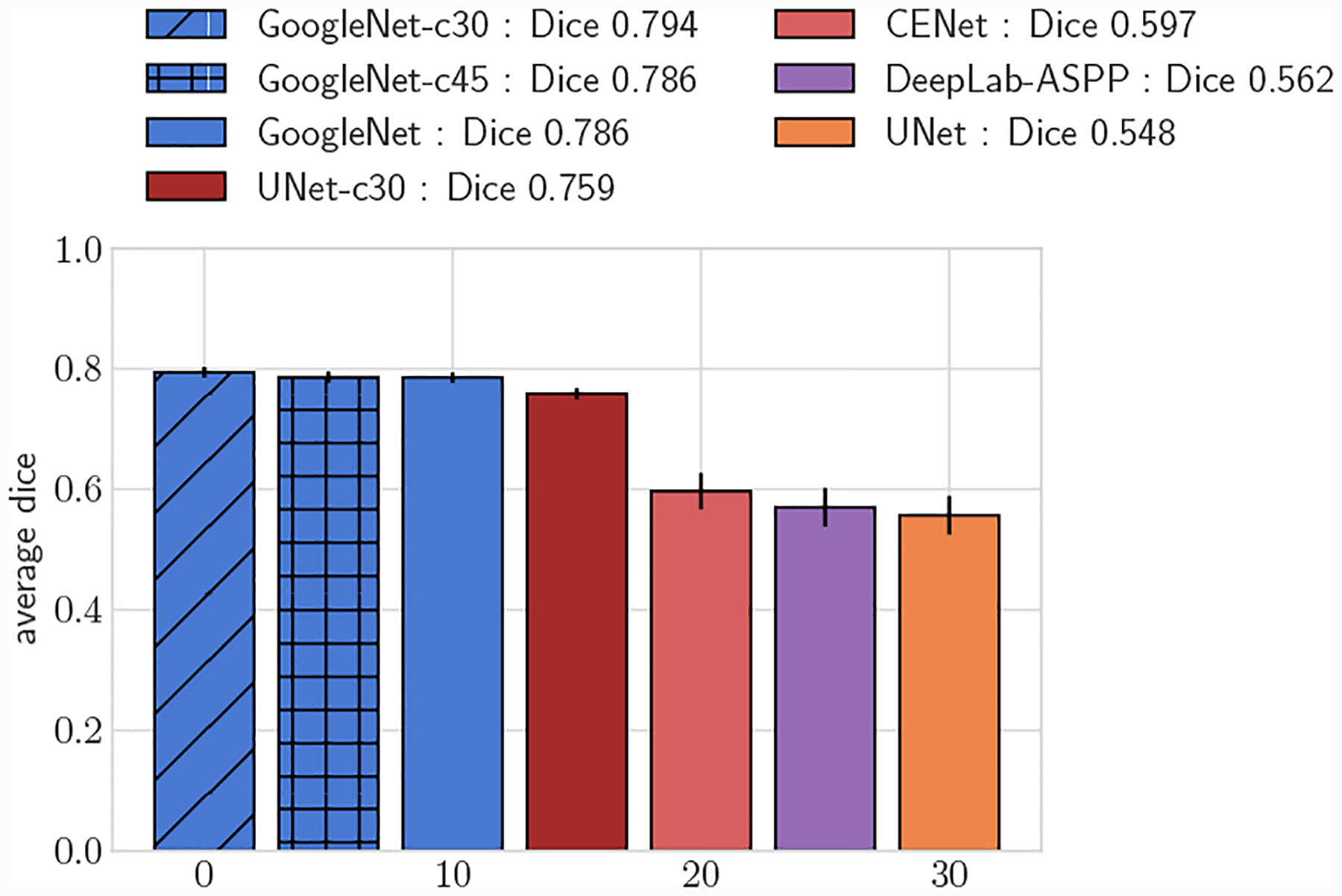
Comparison of UNet lumen regression network to GoogleNet-c30 and segmentation networks. Average DICE for test set, small vessels (r ≤ 0.4cm)

Table 3:

Native minimum image resolution for each image in User Uncertainty Test.

Image	Resolution (cm/pixel)
Cerebro	0.0488
AAA	0.0547
KDR	0.0248
Pulmonary	0.0498

References

- 1.Antiga L, Piccinelli M, Botti L, Ene-Iordache B, Remuzzi A, Steinman DA: An image-based modeling framework for patient-specific computational hemo-dynamics. Medical & Biological Engineering & Computing 46 (2008) [DOI] [PubMed] [Google Scholar]
- 2.Becker C, Rigamonti R, Lepetit V, Fua P: Supervised Feature Learning for Curvilinear Structure Segmentation. Medical Image Computing and Computer Assisted Intervention (2013) [DOI] [PubMed] [Google Scholar]
- 3.Benmansour F, Cohen L: Tubular Structure Segmentation Based on Minimal Path Method and Anisotropic Enhancement. International Journal of Computer Vision 92 (2011) [Google Scholar]
- 4.Chen H, Dou Q, Yu L, Qin J, Heng PA: VoxRes-Net: Deep voxelwise residual networks for brain segmentation from 3d MR images. NeuroImage 170, 446–455 (2018). DOI 10.1016/j.neuroimage.2017.04.041 [DOI] [PubMed] [Google Scholar]
- 5.Chen LC, Papandreou G, Kokkinos I, Murphy K, L. YA: DeepLab: Semantic Image Segmentation with Deep Convolutional Nets, Atrous Convolution, and Fully Connected CRFs. arXiv (2016) [DOI] [PubMed] [Google Scholar]
- 6.Doost SN, Ghista D, Su B, Zhong L, Morsi YS: Heart Blood Flow Simulation: a Perspective Review. Biomedical Engineering Online 15 (2016) [DOI] [PMC free article] [PubMed] [Google Scholar]
- 7.Dou Q, et al. : 3d deeply supervised network for automated segmentation of volumetric medical images. Medical Image Analysis 41, 40–54 (2017). DOI 10.1016/j.media.2017.05.001 [DOI] [PubMed] [Google Scholar]
- 8.Frangi A, Niessen W, Vincken K, Viergever M: Multiscale vessel enhancement filtering. Medical Image Computing and Computer-Assisted Intervention (1998) [Google Scholar]
- 9.Friman O, Hindennach M, Kuhnel C, Peitgen HO: Multiple Hypothesis Template Tracking of Small 3D Vessel Structures. Medical Image Analysis 14 (2010) [DOI] [PubMed] [Google Scholar]
- 10.Grady L: Multilabel Random Walker Image Segmentation Using Prior Models In: 2005 IEEE Computer Society Conference on Computer Vision and Pattern Recognition (CVPR’05), vol. 1, pp. 763–770. IEEE, San Diego, CA, USA: (2005). DOI 10.1109/CVPR.2005.239 [DOI] [Google Scholar]
- 11.Gu Z, Cheng J, Fu H, Zhou K, Hao H, Zhao Y, Zhang T, Gao S, Liu J: Ce-net: Context encoder network for 2d medical image segmentation. arXiv (2019) [DOI] [PubMed] [Google Scholar]
- 12.He K, Zhang X, Ren S, Sun J: Delving Deep into Rectifiers: Surpassing Human-Level Performance on ImageNet Classification. International Conference on Computer Vision (2015) [Google Scholar]
- 13.Heidenreich P, et al. : Forecasting the future of cardiovascular disease in the United States: A policy statement from the American Heart Association. Circulation 123 (2011) [DOI] [PubMed] [Google Scholar]
- 14.Hoogi A, Subramaniam A, Veerapaneni R, Rubin DL: Adaptive Estimation of Active Contour Parameters Using Convolutional Neural Networks and Texture Analysis. IEEE Transactions on Medical Imaging 36 (2017) [DOI] [PMC free article] [PubMed] [Google Scholar]
- 15.Hornik K: Approximation capabilities of multilayer feedforward networks. Neural Networks 4 (1991) [Google Scholar]
- 16.Kamnitsas K, et al. : Efficient multi-scale 3d cnn with fully connected crf for accurate brain lesion segmentation. Medical Image Analysis (2016) [DOI] [PubMed] [Google Scholar]
- 17.Kerrien E, Yureidini A, Dequidt J, Duriez C, Anxionnat R, Cotin S: Blood vessel modeling for interactive simulation of interventional neuroradiology procedures. Medical Image Analysis 35 (2017) [DOI] [PubMed] [Google Scholar]
- 18.Khlebnikov R, Figueroa C: Crimson: Towards a software environment for patient-specific blood flow simulation for diagnosis and treatment. Clinical Image-Based Procedures. Translational Research in Medical Imaging (2016) [Google Scholar]
- 19.Kingma D, Ba J: Adam: A method for stochastic optimization. International Conference on Learning Representations (2015) [Google Scholar]
- 20.Kretschmer J, Godenschwager C, Preim B, Stamminger M: Interactive patient-specific vascular modeling with sweep surfaces. IEEE Transactions on Visualization and Computer Graphics 19 (2013) [DOI] [PubMed] [Google Scholar]
- 21.Krissian K, Malandain G, Nicholas A: Model-Based Detection of Tubular Structures in 3D Images. Computer Vision and Image Understanding 80 (2000) [Google Scholar]
- 22.Law MWK, Chung ACS: Three Dimensional Curvilinear Structure Detection Using Optimally Oriented Flux. European Conference on Computer Vision (2008) [Google Scholar]
- 23.Law MWK, Chung ACS: An oriented flux symmetry based active contour model for three dimensional vessel segmentation. European Conference on Computer Vision (2010) [Google Scholar]
- 24.LeCun Y, Bengio Y, Hinton G: Deep learning. Nature 521 (7553), 436–444 (2015). DOI 10.1038/nature14539 [DOI] [PubMed] [Google Scholar]
- 25.Lesage D, Angelini E, Bloch I, Funka-Lea G: A review of 3D vessel lumen segmentation techniques: Models, features and extraction schemes. Medical Image Analysis 13 (2009) [DOI] [PubMed] [Google Scholar]
- 26.Lorigo LM, et al. : CURVES: Curve Evolution for Vessel Segmentation. Medical Image Analysis 5 (2001) [DOI] [PubMed] [Google Scholar]
- 27.Maher GD, Wilson NW, Marsden AL: Accelerating Cardiovascular Model Building with Convolutional Neural Networks. Medical and Biological Engineering and Computing (2019) [DOI] [PMC free article] [PubMed] [Google Scholar]
- 28.Marsden A: Simulation based planning of surgical interventions in pediatric cardiology. Physics of Fluids 25 (2013) [DOI] [PMC free article] [PubMed] [Google Scholar]
- 29.Merkow J, Marsden A, Kriegman D, Tu Z: Dense volume-to-volume vascular boundary detection In: Medical Image Computing and Computer-Assisted Intervention. Springer International Publishing, Cham: (2016) [Google Scholar]
- 30.Merkow J, Tu Z, Kriegman D, Marsden A: Structural edge detection for cardiovascular modeling In: MICCAI 2015, pp. 735–742. Springer; (2015) [Google Scholar]
- 31.Moreno R and Smedby Ö: Gradient-based enhancement of tubular structures in medical images. Medical Image Analysis 26 (2015) [DOI] [PubMed] [Google Scholar]
- 32.Petersen K, Schaap M, Lesage D, Lee M, Grady L: Fast and Accurate Segmentation of Coronary Arteries for Improved Cardiovascular Care. GPU Technology Conference p. 55 (2017) [Google Scholar]
- 33.Pezold S, et al. : Automatic, Robust, and Globally Optimal Segmentation of Tubular Structures. Medical Image Computing and Computer Assisted Intervention (2016) [Google Scholar]
- 34.Ronneberger O, Fischer P, Brox T: U-net: Convolutional networks for biomedical image segmentation. In: Medical Image Computing and Computer Assisted Intervention (2015) [Google Scholar]
- 35.Rudyanto R, et al. : Comparing algorithms for automated vessel segmentation in computed tomography scans of the lung: the vessel12 study. Medical Image Analysis 18 (2014) [DOI] [PMC free article] [PubMed] [Google Scholar]
- 36.Sankaran S, Kim H, Choi G, Taylor C: Uncertainty quantification in coronary blood flow simulations: Impact of geometry, boundary conditions and blood viscosity. Journal of Biomechanics 49 (2016) [DOI] [PubMed] [Google Scholar]
- 37.Schaap M, et al. : Standardized Evaluation Methodology and Reference Database for Evaluating Coronary Artery Centerline Extraction Algorithms. Medical image analysis 13 (2009) [DOI] [PMC free article] [PubMed] [Google Scholar]
- 38.Schmidhuber J: Deep learning in neural networks: An overview. Neural Networks 61, 85–117 (2015). DOI 10.1016/j.neunet.2014.09.003 [DOI] [PubMed] [Google Scholar]
- 39.Schumann C, Neugebauer M, Bade R, Preim B, Peitgen H: Implicit vessel surface reconstruction for visualization and CFD simulation. International Journal of Computer Assisted Radiology and Surgery 2 (2008) [Google Scholar]
- 40.Szegedy C, et al. : Going Deepr with Convolutions. Convference on Computer Vision and Pattern Recognition (2015) [Google Scholar]
- 41.Taha AA, Hanbury A: Metrics for Evaluating 3D Medical Image Segmentation: Analysis, Selection and Tool. BMC Medical Imaging 15 (2015) [DOI] [PMC free article] [PubMed] [Google Scholar]
- 42.Taylor C, Figueroa C: Patient-specific Modeling of Cardiovascular Mechanics. Annual Review of Biomedical Engineering 11 (2009) [DOI] [PMC free article] [PubMed] [Google Scholar]
- 43.Updegrove A, Wilson N, Merkow J, Lan H, Marsden A, Shadden S: SimVascular: An Open Source Pipeline for Cardiovascular Simulation. Annals of Biomedical Engineering 61 (2013) [DOI] [PMC free article] [PubMed] [Google Scholar]
- 44.Updegrove A, Wilson N, Shadden S: Boolean and smoothing of discrete surfaces. Advances in Engineering Software 95 (2016) [Google Scholar]
- 45.Urick B, M. ST, Hossain SS, Zhang YJ, Hughes TJR: Review of patient-specific vascular modeling: Template-based isogeometric framework and the case for cad. Archives of Computational Methods in Engineering 26 (2019) [Google Scholar]
- 46.Wang KCY: Level set methods for computational prototyping with application to hemodynamic modeling. Ph.D. thesis, Stanford University; (2001) [Google Scholar]
- 47.Wilson N, Ortiz A, Johnson A: The Vascular Model Repository: A Public Resource of Medical Imaging Data and Blood Flow Simulation Results. Journal of Medical Devices 7 (2013) [DOI] [PMC free article] [PubMed] [Google Scholar]
- 48.Wolterink JM, Leriner T, Isgum I: Graph convolutional networks for coronary artery segmentation in cardiac ct angiography. arXiv (2020) [Google Scholar]
- 49.Xie E, Sun P, Song X, Wang W, Liang D, Shen C, Luo P: Polarmask: Single shot instance segmentation with polar representation. arXiv (2020) [Google Scholar]
- 50.Zhang Y, Bazilevs Y, Goswami S, Bajaj C, Hughes T: Patient-specific vascular NURBS modeling for isogeometric analysis of blood flow. Computer Methods in Applied Mechanics and Engineering 196 (2007) [DOI] [PMC free article] [PubMed] [Google Scholar]