Abstract
There have been many improvements and advancements in the application of neural networks in the mining industry. In this study, two advanced deep learning neural networks called recurrent neural network (RNN) and autoregressive integrated moving average (ARIMA) were implemented in the simulation and prediction of limestone price variation. The RNN uses long short-term memory layers (LSTM), dropout regularization, activation functions, mean square error (MSE), and the Adam optimizer to simulate the predictions. The LSTM stores previous data over time and uses it in simulating future prices based on defined parameters and algorithms. The ARIMA model is a statistical method that captures different time series based on the level, trend, and seasonality of the data. The auto ARIMA function searches for the best parameters that fit the model. Different layers and parameters are added to the model to simulate the price prediction. The performance of both network models is remarkable in terms of trend variability and factors affecting limestone price. The ARIMA model has an accuracy of 95.7% while RNN has an accuracy of 91.8%. This shows that the ARIMA model outperforms the RNN model. In addition, the time required to train the ARIMA is than that of the RNN. Predicting limestone prices may help both investors and industries in making economical and technical decisions, for example, when to invest, buy, sell, increase, and decrease production.
Keywords: Limestone, Recurrent neural network, Long short-term memory, Autoregressive integrated moving average, Price, Predict
Introduction
Limestone plays a vital role in the world. Limestone is a special type of sedimentary rock. It makes up about 10% of the earth’s sedimentary rocks. According to research, about 25% of the world’s population derives their water from limestone and about 50% of oil and gas reserves are trapped in limestone rocks [38]. Limestone is mainly formed by the deposition of sediments and biomineralization. It is commonly found around the surface of the earth. Limestone is found in many parts of the world. China alone produces about 62% of the world’s limestone, followed by Europe, the USA, and Japan [30]. Previous studies forecast that the consumption of limestone will grow by 2% annually. Limestone is used as a raw material in the production of cement, tiles, lime steel production, the treatment of waste, and other products (Håkan [25, 27]). Limestone can also be used in the agricultural sector and in the treatment of glass [23]. Limestone serves as a raw material for many other downstream industries [13]. The demand for limestone is expected to increase by 6% in the construction industry and to find an application in water treatment [36]. According to the World Water Report in 2018, the consumption of water increased by 1% every year due to the increase of economic development and growth in population [26]. Despite the fact that the price of limestone is relatively low compared to other mining products such as gold, silver, and diamonds, its price in the world market undervalues its true economic importance.
There are many factors which affect the production and the prices of limestone. Edward and Samuel suggested that the four main factors affecting limestone production are the location (proximity to good market, infrastructures such as roads, energy, and delivery), the grade of the limestone, the closeness to the surface, and a cheaper labor force [23].
Most scholars argue that one of the main factors affecting the prices of limestone is competition. Competition is defined by a number of factors such as the market, cheap labor, quality, accessibility, energy, and even the location of the mine [51]. Competition may occur at any stage during production or at the market level (production rate, selling price, and demand and supply). Jessica et al. suggested that one of the main causes of competition is oversupply by the entry of new suppliers which causes competitiveness in the stock market [32].
One important factor that can directly influence the prices of limestone is the energy used during mining and processing. Energy has a positive correlation with limestone prices. An increase in energy prices will lead to an increase in the prices of limestone and vice versa. According to National Stone, Sand and Gravel Association (NSSGA), and the Natural Stone Council (NSC), major energies used in mining and processing of limestone are electricity, coal, gasoline, natural gas, liquid fuel, and renewable energy [24, 49]. According to the U.S. Energy Administration, liquid fuel accounts for 29.4%, coal 25.2%, natural gas 22.9%, electricity 15.1%, and renewable energy 7.4% of industrial energy consumption in the world [50].
Another factor that may influence the limestone market is the demand by construction industries. Limestone is used by the construction industries to build houses, roads, railways, dams, and other infrastructures. According to the Institute of Civil Engineering (ICE), the construction industry is expected to reach about $8 trillion globally. An increase in the construction industry will lead to an increase in the demand for limestone. Limestone is also used as a raw material in the production of cement. An increase in the prices of limestone will lead to an increase in the prices of cement and vice versa.
Gold is used as a store for wealth which can indirectly influence limestone prices. Gold can influence market prices in terms of inflation, uncertainty, and interest rates. For example, when inflation increases, the demand for gold increases as the real value of currencies decreases; investors tend to buy more gold to preserve their wealth rather than investing in other products such as limestone [55]. Unlike inflation, interest rates have a negative relationship with gold. An increase in interest rates will lead to a decrease in the prices of gold. An increase in interest rates is usually caused by a growing economy where investors tend to invest in different sectors as the demand and supply of other products increases. A growing economy will therefore lead to a boom in agricultural and construction industries which uses limestone as a raw material. A decrease in interest rates leads to an increase in gold prices since investors tend to safe haven their wealth in the form of gold to prevent them from currency devaluation and a decrease in demand and supply of other goods and services. Interest rates can also be influenced by the stock market. For example, if interest rates increase, producers will increase their production to benefit from the increase in interest rates and vice versa [16].
The prediction of limestone prices may depend on the supply and demand of limestone (uses and production per industry), the energy used during its production, the grade (high-grade limestone is more expensive than low-grade limestone), the interest rates, and location. The location of the mine can affect both the cost of production and the cost of selling. The cost of production can be cheaper in some areas than others as such leads to a low cost of limestone ([37]; Batavia, 3 Factors Influencing the Cost of Crushed Limestone, [5–10]; Dixon, Milling Practice of the Kirkland Gold Mines, [21]). In this study, six factors affecting the limestone market were selected to simulate and predict future limestone price trends. The six factors are cement, gold, coal, energy, interest rates, and limestone prices. Data from the different factors influencing limestone price variations were collected for a period of 6 years.
There are many articles about predictions in the mining industries due to their importance and value to society. Some of which are predicting the prices of valuable ore, predicting mining operations such as the strength of rocks, blasting, rock/ore, and composition. A valid prediction of ore prices may help both investors and the manufacturing industries. Investors can know when to buy and sell their shares while manufacturing industries can know how to regulate their production to meet up with the demand. In the same way, predictions in mining operations can provide a safe ground for certain operations. For example, predicting the strength of rock can help engineers to design and conduct safe operations such as slope angle design, blasting parameters, and rock support.
It is much easier to predict the price of gold than limestone. Gold has once been used as a monetary standard, “The Classical Gold Standard,” where all currencies were linked to a specified amount of gold [56]. In 2011, the Malaysians used the gold over paper currency because it had a more stable monetary value [29]. Gold has been used as a medium of exchange throughout history [34]. Gold is used in supporting transactions [45]. This makes the prediction of gold prices easier to predict. Changes in gold prices can cause a change in other product prices which already have an equivalency, especially in the stock market. On the other hand, very little research has been conducted on predicting the prices of limestone. There are a few articles which have implemented neural networks in limestone operations. Some of these include the prediction of blast patterns in limestone quarries [48], prediction of oil recovery efficiency in limestone cores [11], and the prediction of compressive strength of limestone [3].
The predictions of mining products have gained popularity over the years and have led to the evolution of techniques and methods used in making the predictions. Previous studies show that there are many factors such as variables, parameters, indicators, programming languages, software, and network models which can greatly influence the results of price prediction. There are many different types of neural networks that have been implemented in predicting prices and other operations. For example, artificial neural network (ANN), convolutional neural network (CNN), autoencoders (AE), Boltzmann machine (BM), extreme learning machine (ELM), and autoregressive integrated moving average (ARIMA) have been used for price predictions in the mining industry. The concept behind deep learning is that these networks try to mimic the human brain. The CNN is associated with the occipital lobe, the ANN is the temporal lobe, and the RNN is the frontal lobe which is the largest part of the brain and is also responsible for long short-term memory. This is a very important factor in predicting prices as the network remembers previous values and can compute future values based on the previous value accuracy [1]. Some research has implemented both ANN and ARIMA in price predictions [18]. Kuma et al. achieved 93% accuracy using EML and made a contrast between EML and feed-forward neural network (FFNN) with and without backpropagation [17]. Ismail et al. implemented multiple linear regression (MLR) in the price prediction of gold price-based economic factors and on eight variables which resulted in 96.92% accuracy [31]. Neural networks have also been implemented on different limestone operations such as predicting cement price [53] and predicting geological properties of limestone [4].
In this study, RNN and ARIMA were used to simulate and predict future prices of limestone.
ARIMA is one of the most complex network models in predictions, but if well modeled, it can produce very good results. The ARIMA model is flexible and based on a number of parameters that can be tuned automatically to obtain better results. The ARIMA model addresses the problem in terms of stationarity, seasonality, regression, and moving average [14]. It combines a set of complex parameters such as autoregression (AR), integrated (I), and moving average (MA). The AR takes into consideration the differences between the lag observations (p). A lag is essentially a fixed amount of passing time. The lag observations are created by shifting the time series (prices of limestone) in steps. The new values created by this shift in steps are called the lag time series and can be used to create autocorrelation by comparing it to the original prices of limestone. The I parameter is responsible for the data type (stationary and non-stationary), ensuring all data types are stationary. The MA calculates the average error between lag observations (q) [46]. The ARIMA model is denoted as p, d, and q, which are the fundamental parameters of the network. The parameters p, d, and q can also be referred to as non-seasonal data types of the ARIMA model. Non-seasonal data has no regular pattern of change over a certain period of time while seasonal data has regular pattern change over a certain period of time. The easiest way to model seasonal prediction is to calculate the parameters by plotting the data against time and measure the linearity by using the autocorrelation function. The ARIMA model identifies the differences in trend, seasonality, lag size, coefficient of regression, and error difference. Contrary to other ARIMA models which uses a specific data or data that has been created to demonstrate a particular parameter or hypothesis, the model implemented in this study was adapted to produce good results with a real-life data. Most ARIMA models focus on finding the 3 ARIMA parameters (p, d, and q), integrated (I), and moving average (MA) models; the model implemented in this study goes way beyond that. For example, this model shows the conversion of non-stationary data to a stationary data, the use of multiple differencing and decomposition to stabilize the data, calculation of error using symmetric mean absolute percentage error, diagnosing using standardized residuals, correlogram, histograms, and autocorrelation plots as described in Section 3.3 below.
The recurrent neural network uses a stochastic gradient descent to train deep learning neural networks [15]. The layers are connected by neurons through time [39]. In the RNN, the information travels through time, previous information is used as input for the next point, and the cost function can be calculated at each point [42]. There are two main problems associated with recurrent neural network, the vanishing gradient problem, and the exploding gradient. These problems can be solved by implementing long short-term memory (LSTM). The LSTM structure is made up of the input layers (gray), the hidden layers (blue), and the output layers (green) (Fig. 1). The LSTM neurons have memories within their pipeline that can store previous information, update the information, and pass it to the next layer or cell without losing information [39]. In addition, LSTM models update complexity per weight and time step [28]. Despite the complexity of LSTM, its performances far outweigh its shortcomings when implemented correctly. Cho et al. proposed a gated recurrent unit variant to solve the vanishing gradient problem. The GRU uses an updated gate which consists of the single gate and the forget gate. It also combines the cell state and hidden state together with other changes to make the model simpler [19]. Unlike other models, the RNN in this study was modeled to overcome many problems faced by most machine learning (ML) methods. Some of these problems are dimensionality reduction, vanishing gradient problem (described above), overfitting/underfitting, long run times, pattern recognition, and hyperparameters optimization. More about this is described in Section 3.2 below.
Fig. 1.
LSTM structure showing input layers, hidden layers, and output layers
The main objective of this study was to model the price variation of limestone. With respect to this, two powerful network models (RNN and ARIMA) recommended by most researchers were implemented in the prediction of price variation. The models were investigated in terms of flexibility, accuracy, and error minimization based on the dataset used.
Data Preprocessing
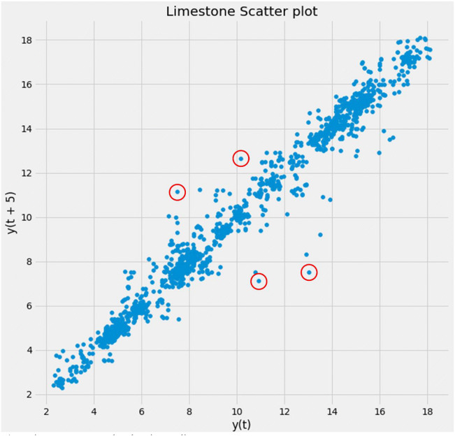
The data used in this study is the historical data of limestone prices for a period of 6 years from January 2014 to April 2020. The data was downloaded from Yahoo Finance, Eoddata, Marketwatch, Indexmundi, and Statista. The preprocessing of the data is an important step in ML. The data may greatly affect the results of a network model, especially when dealing with real-world problems. Some of the problems that real-world data can have are missing values, outliers, types, formats, and seasonality. Outliers are data that are in an abnormal position (random position) with the rest of the dataset. It can easily be identified by visualizing a scatter plot of the dataset as shown in Fig. 2. In Fig. 2, the x-axis is represented in the graph as y(t) while the y-axis is represented as y(t+5). The y(t) is the original value of limestone recorded at time y(t) while the y(t+5) is the value of limestone recorded at time y(t+5) that is shifted by five of the time series. In this case, the difference between lag1 and lag5 is not much which means that the daily prices between each day are not much. Also, the data shows an identifiable pattern of linear correlation. The data is cleaned by filling in missing values by calculating the mean of the interval. The data is normalized to avoid unbiased situations Eq. (1). Normalizing input data in the range of (0,1) gives the data equal weight or importance. The advantage of using normalization over standardization is that it has smaller standard deviations which can help to suppress the effect of outliers [20]. It is also recommended to use normalization, especially when using the activation function in the output layer of the recurrent neural network.
Fig. 2.
Limestone scatter plot showing outliers
| 1 |
Correlation of Factors Affecting Limestone Prices
Correlation analysis is conducted on factors affecting the price of limestone (price of cement, gold, coal, energy, and interest rates). Correlation is a statistical measure of the relationship strength between two or more variables. The correlation coefficient (CC) of the data is calculated using the CORREL function in Microsoft Office Excel. The correlation results are recorded in Table 1. CC of − 1 indicates a negative correlation, CC of + 1 indicates a positive correlation, and a CC of near 0 indicates no correlation. From the correlation results, it can be seen that the correlation coefficient of a different factor against themselves shows a perfect positive correlation of 1. The correlation coefficient between gold and limestone is 0.59, which also shows a positive correlation. An increase in the prices of gold will also lead to an increase in the prices of limestone and vice versa. The prices of the gold increase due to uncertainty during inflation and investors tend to purchase gold as a safe haven. Gold can be used as a hedge during inflation, political instability, or currency devaluation [44]. During uncertainty, investors look for other mining commodities to invest their money in by buying more limestone stock to safe haven their wealth. They can make a higher profit after inflation when prices will go up even higher. Another reason may be that during uncertainty, the value of the real estate and other commodities produced from limestone may fall, which may affect the production of limestone. A decrease in the production of limestone may lead to an increase in the prices of limestone due to scarcity. Coal and energy have negative correlations to limestone. This shows that limestone is not directly affected by the change in the prices of energy used during production. Also, the prices of energy may vary in different locations. Some other factors (cost of production, labor force, equipment, and operations) may also vary in different locations. On the other hand, cement, which is produced from limestone, shows a positive correlation of 0.65. This means that an increase in limestone will lead to an increase in the production of cement and vice versa. During an economic boom, real estate stocks will rise higher and the demand for raw materials like limestone will also increase leading to an increase in the prices of limestone. Conclusively, the change in the prices of limestone is not directly affected by the energy needed during production but by other factors such as the market, demand, financial, political, and economic factors.
Table 1.
Correlation coefficient of factors affecting limestone prices
| Price increase | Limestone | Gold | Energy | Coal | Cement | Interest rates |
|---|---|---|---|---|---|---|
| Price | ||||||
| Limestone | 1 | |||||
| Gold | 0.59 | 1 | ||||
| Energy | − 0.51 | − 0.74 | 1 | |||
| Coal | − 0.49 | − 0.84 | 0.84 | 1 | ||
| Cement | 0.65 | 0.17 | 0.08 | − 0.03 | 1 | |
| Interest rates | 0.86 | 0.57 | − 0.34 | − 0.41 | 0.75 | 1 |
Modeling of Limestone Prices
Two different network models are used in this study: the RNN and ARIMA model. The dataset is divided into a training set and a test set. The training set is used to train the network model while the test set is used to validate the predictions.
The RNN Model
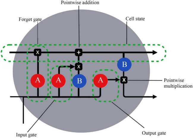
The RNN model is a network model that is able to learn data patterns during training, stores important information, and uses it in predictions. Based on its limitations, like short sequences and computational resources, variants of RNN have been developed to overcome these problems. Some of the variants are LSTM and GRU. The LSTM model uses a sequential time series and a stochastic approximation process [22]. The sequential model is used to add multiple LSTM layers to the network that captures the upward and downward trend of the prices. The LSTM is made up of cells. Each cell has an input gate, output gate, forget gate, and a cell state (Fig. 3). The data is first converted as readable vectors and process one after the other. The first vectors processed by the first cells are sent to the next cell by the hidden layers (which function as the network’s memory). In the next cell, the new input and the previous data combine together to form a vector. The vector passes through the activation function where the values are being normalized to 0 and 1 or − 1 and 1. Normalization is important in the sense that it gives equal weights to the data. This means that the magnitude or weight of each feature is more or less the same. Another reason is that normalizing the data will transform it to a mean close to zero (positive and negative values) which is easier to compute than a dataset with all positive values or negative values. The values close to 0 or − 1 are less important and are more likely to go through the forget gate. The values with 1 are more important and are more likely to go through the output gate. Before they go through the output gate, they are combined with the new inputs and pass through the activation function. The new cell state can be determined by multiplying the forget vector to the previous cell state. Values which are near or close to − 1 and 0 are more likely to be dropped. A pointwise addition of the output of the input gate will then determine the cell state. The output can then be used in predictions [43].
Fig. 3.
LSTM cell showing the cell state, input gate, output gate, and forget gate. A and B are activation functions
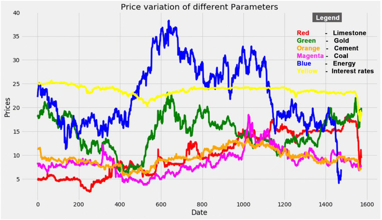
The data was imported and visualized as shown in Fig. 4. From the graph, we can see that the variation pattern of limestone price is represented as red, gold price as green, cement price as orange, coal price as magenta, energy prices as blue, and interest rates as yellow. This variation pattern shows which factors are highly correlated with limestone prices by the upward and downward movement with respect to limestone price variation. The dataset has a total of 1575 points which represents the data collected on a daily basis from January 2, 2014, to April 3, 2020. The data has a total of six factors (limestone, cement, gold, interest rates, coal, and energy). The data of each factor was collected separately for the same amount of time. The mean of each day (mean of high, low, and close) was recorded in the dataset. Feature selection is done by both automatic and manual selection methods. For the manual selection method, the visualization in Fig. 4 can be used to compare which factors or features are closely correlated with limestone while in the automatic selection, (− 1) can be used to find the best values during reshaping. The dataset was scaled (normalized) to the interval of (0, 1) to avoid bias and help the algorithm converge easily. The standard input for the LSTM layer is in the form of a 3D array. The data is then converted into a 3D array. The 3-dimensional array consists of the batch size, time steps, and features. Putting the data into a 3D array helps to reduce the number of features thereby increasing the classifier performance and limit overfitting of the model. This helps to solve the problem of dimensionality.
Fig. 4.
Price variation representation of factors affecting the price of limestone, with respect to date
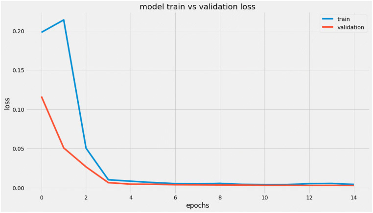
The LSTM layers are added using the sequential model. The grid search is used to tune hyperparameters (activation function, dropout regularization, batch size, number of epochs, neurons in hidden layers, and optimizer.) The data is dispatched in batches known as batch size. The batch size determines the number of patterns that the network receives before weights are updated and stored in the memory. The number of times the training data is fed into the network is known as the epoch. The grid-search method is used to determine the number of a batch size of 40 and 15 epochs (batch size and epochs search code). The grid search is also used to find the best optimizer. In this case, the Adam optimizer produced the best results with respect to the data and shows an accuracy of 87% (optimizer code) [33]. The activation function selects which neuron is activated by summing the input weights and a bias. The ReLU activation was chosen after applying the grid search (activation function code). The ReLU function has a number of benefits due to its nonlinear sparse activation. This means only neurons which meet the threshold criteria will be fired. This is particularly important as many layers can be stacked together without activating all the layers [52]. During the training of the network, dropout regularization is used to drop out certain nodes (excluded from being activated) when the network is saturated to prevent overfitting of the network model. A summary of the model shows that there were 12,131 trainable parameters. The network model was compiled using the Adam optimizer, and the loss of the model was calculated using the mean square error (MSE) function equation (2). Where is the mean, and is the squared difference between the predicted and the actual value. The MSE estimates and updates the weights, thereby decreasing the loss and improving the generalization error [15]. The network model is trained over 15 epochs, a batch size of 40, validation split of 0.1, and dropout regularization of 0.2. Figure 5 shows the loss of the model versus epochs. The loss is the sum of errors of the training set and validation set. The training loss and validation loss decreases to a point of stability, which shows that all the parameters have been tuned optimally. Also, there is no overfitting or underfitting of the model which shows good convergence. This means that the model is well fitted and that the model can give good predictions. The results of the predictions were visualized using Matplot Library. The full code can be found on GitHub.
Fig. 5.
Loss versus epochs shows how well the model fits with respect to the training set and test set
| 2 |
The ARIMA Model
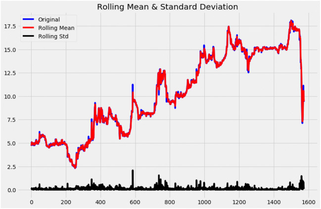
Autoregression integrated moving average (ARIMA) takes into consideration the assumption that the past or previous data can forecast the behavior of present and or future data under normal conditions. The name clearly defines the aspects of the model. It is based on autoregression, integration, and moving average. It uses lag observations to determine the difference in raw observations and calculates error. The main parameters of the ARIMA model are lag order (P), degree of differencing (D), and order of moving average (Q) [12]. Before simulating the model, a scatter plot of the dataset is used to visualize the data as shown in Fig. 2. The scatter plot (lag plot) shows a positive linear correlation with some outliers and randomness. The scatter plot helps to visualize the data and to determine what type of model is suitable for the data. In this case, the scatter plot is linear, so the use of an autoregressive model will be a good choice for predictions [47]. The Dickey-Fuller test (DFT) is used to test for stationarity in the data. The dataset is said to be stationary when certain statistical properties are constant and have an independent covariance. This is particularly important as most statistical analysis works best on stationary data. Also, stationary datasets are easier to model, especially in time series analysis. From the DFT test, it can be seen that the dataset is not stationary (non-stationary) by the upward and downward movement of the rolling mean and standard deviation as shown in Fig. 6. Also, the static test is more than 5% of critical value and the p value (0.49) is greater than 0.05. So, the Dickey-Fuller null hypothesis cannot be rejected. Before diving into the predictions, the dataset needs to be transformed into a stationary data in order to have good results of the prediction. A non-stationary data can be converted to a stationary data by applying decomposition and differencing techniques [41]. Decomposition is the separation of the trend and seasonality of the dataset. Differencing is finding the differences of the observations as shown in the code section of the ARIMA model. Once it is converted into a stationary data, the auto ARIMA function is used to find the best values of p, d, and q (ARIMA hyperparameters code). The (p) parameter stands for the order of the autoregressive model, the (d) parameter stands for the order of differencing, and the (q) parameter stands for the order of the moving average. The (p) parameter uses past values in regression calculations, and the (d) parameter subtracts the previous and current values of (d). The (d) parameter is also used to convert the data from non-stationary to a stationary data. The (q) parameter defines the error of the model by a combination of previous errors. It determines the number of terms to be included in the model. After fitting the model, the optimal values of p, d, and q were (0, 1, 2) which can be written as equation (3) where μ is the regressive parameter, Yt − 1 the differencing, and θ1 et − 1 the moving average.
Fig. 6.
Dickey-Fuller test for stationarity showing upward and downward movement of rolling mean and standard deviation
| 3 |
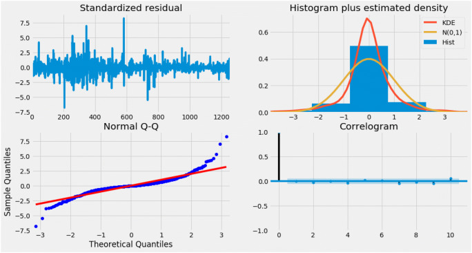
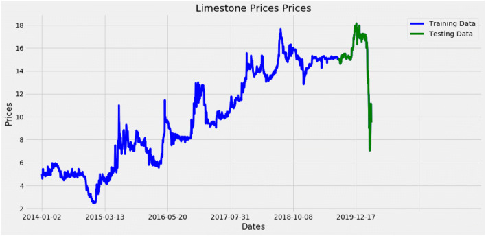
The diagnostic plots are used to visualize the auto ARIMA model. Figure 7 shows four graphs. At the top left corner, standardized residuals fluctuate around a mean of zero. The top-right displays the density plot which shows a normal distribution. The bottom left represents a correlation which shows a normal liner distribution following the red line. Lastly, the bottom right is the ACF (correlogram) which shows that the residuals are not autocorrelated. From the diagnosis, auto ARIMA will fit the data perfectly. An ARIMA model is then created with the optimal parameters of p, d, and q (ARIMA model evaluation). The dataset is divided into a training set (used to train the model) and a test set (used to compare and validate the predictions) as shown in Fig. 8. Of the data, 80% is used for the training set and 10% is used for the test set. The symmetric mean absolute percentage error (SMAPE) Eq. (4) is used to evaluate the model [54]. In Eq. (4), At is the actual value and Pt is the predicted value. It is calculated by differencing the absolute of the actual value from the absolute of the predicted value divided by half the sum of the predicted and actual values. The result is summed for each fitted point (t) and divided by the number of fitted points (n) [35]. This equation evaluates the model by generating a positive and negative error while limiting the effect of outliers and bias [2].
Fig. 7.
Auto ARIMA plot diagnostics
Fig. 8.
Training set and test set. The training set is used to train the network while the test set is used to validate the predictions
The prediction is done by using the predict function (interprets the number of features it receives from the model and passes the number of features it receives to the output layer) of the future price range. The full code can be found on GitHub.
| 4 |
Results and Discussion
The two network models show a tremendous performance in price prediction. The loss is calculated by the MSE for the RNN model and SMAPE for the ARIMA model.
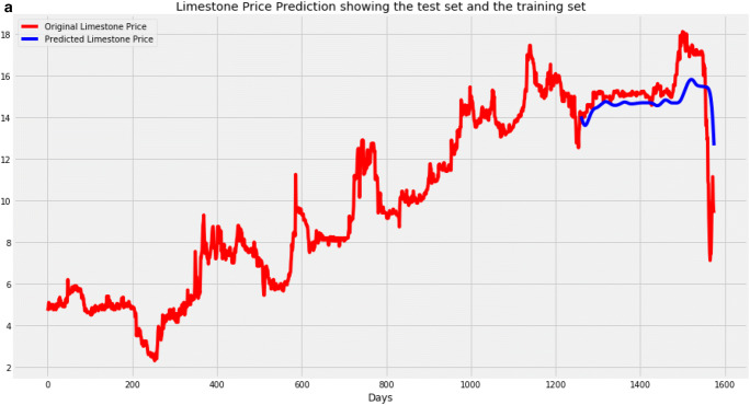
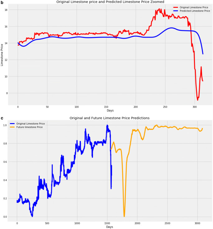
Two predictions are done for the RNN model. The first predictions are compared with the test set to see how well the model predicted the test set. The second predictions are future predictions. There is no data available to compare the second prediction. Figure 9a, b, c show the results of the RNN model. Figure 9a shows the results of the training set, the test set, and the predicted price. In Fig. 9b, only the test set and the predicted prices are displayed. Figure 9c shows the original data and future predictions. The test set is in red, the predicted price is in blue, and the future predictions are in orange. From the results of Fig. 9a, b, and c, the RNN model predicts the upward and downward movement of prices to an extent but is unable to capture the exact prices at certain intervals. Also, the future predictions begin with a visible upward and downward movement of the graph but later become almost horizontal as the predictions go further into the future. This may mean that the future predictions are more accurate the closer they are to the present, but they are less accurate the farther into the future.
Fig. 9.
a RNN results of test set and predicted limestone prices. b RNN results of test set and predicted limestone prices zoomed. c RNN results of the original dataset and future predictions
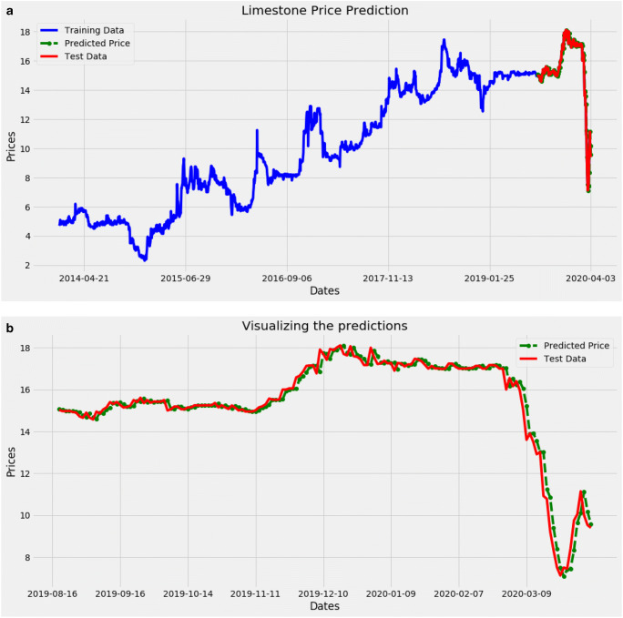
Figure 10a and b show the results of the ARIMA model. Figure 10a shows all results of the training set, test set, and the predicted limestone prices. In Fig. 10b, only the test set and the predictions are displayed. The training set is in blue, the test set is in red, and the predicted limestone prices are in green. From the graph, it can be seen that the ARIMA model predicts almost the same price as the test set. It follows the upward and downward movement of the graph.
Fig. 10.
a ARIMA results showing training set in blue, test set in red, and predicted limestone prices in green. b Visualizing the ARIMA model predictions, the test set is in red, and the predictions in green
From the results, the ARIMA model displays better predictions than the RNN model. Also, the ARIMA model uses less training time as compared to the RNN model. The RNN model shows an accuracy of 91.8% while the ARIMA model shows an accuracy of 95.7%. The ARIMA model is more accurate than the RNN model. This may be due to the auto ARIMA function used to find the best possible values of p, d, and q. The poor results in the RNN model may be due to the fact that some of the hyperparameters were tuned manually. For example, the number of LSTM layers was tuned manually.
Analysis from the results shows that there has been a steady increase in the prices of limestone from 2014 until the beginning of 2020. This is in accordance with the literature review in Section 1 which states that the limestone market is expected to rise about 2% annually. The sharp decrease in the year 2020 may be due to the coronavirus (COVID-19) which pushed most industries to shut down in order to prevent the spread of the virus. Due to the fact that most of these industries were shut down, it affected the production and consumption of limestone as seen on the graphs in the early months of 2020. According to the Brownian motion, the state of future variations (price) is a stochastic process determined by a collection of random variables [40]. This means that the future variations of an ore price may vary from the past and may be difficult to predict the exact price due to variations that may occur in the future. However, if the variables of a model are well tuned based on a given circumstance and assumptions, it can produce accurate results.
Conclusions
Limestone is a very important raw material for many industries. Its production and consumption are very important to the economy and in daily use. Predicting limestone prices can be beneficial to investors as it can help them know when to invest and when to sell their stock. It can also help production industries to regulate their production rates and market prices. Choosing the right network model in predictions is very crucial as the results may have a great impact on industries and investors. In this study, two deep neural network models ARIMA and RNN were used to predict limestone prices. Despite their complexity in modeling, the results were encouraging. According to the results, the ARIMA model predictions were better than the RNN model in terms of the trend and variation of limestone prices. The main difference between these two models lies in the fact that the ARIMA model is able to produce more accurate results than the RNN model. Also, the training time of the ARIMA model is less compared to the training time in the RNN model. This may be due to multiple LSTM layers. The ARIMA network is proven to be a sophisticated method in modeling, analyzing, and predicting prices.
This study presents a simple yet sophisticated means of applying deep learning algorithms to mining economics. The authors intend to implement deep learning in mining operations. The next sections to follow will be implementing deep learning neural networks in scheduling, simulation of economics, and technical parameters to solve complex problems.
Compliance with Ethical Standards
Conflict of Interest
The authors declare that they have no conflict of interest.
Footnotes
Publisher’s Note
Springer Nature remains neutral with regard to jurisdictional claims in published maps and institutional affiliations.
Contributor Information
Tawum Juvert Mbah, Email: juvertmbah@whut.edu.cn.
Haiwang Ye, Email: yehaiwang369@hotmail.com.
Jianhua Zhang, Email: zjhwut@sina.com.cn.
Mei Long, Email: 584763031@qq.com.
References
- 1.Andrej K, Johnson J, Fei-Fei L (2016) Visualizing and understanding recurrent networks. Stanford University, ICLR. http://vision.stanford.edu/pdf/KarpathyICLR2016.pdf
- 2.Armstrong JS, Fildes R (1979) Long-range forecasting: from crystal ball to computer, 1st edn. Wiley
- 3.Ayatl H, Kellouchel Y, Ghrici M, Boukhatem B (2018) Compressive strength prediction of limestone filler concrete using artificial neural networks. Adv Comput Des 3:289–302. 10.12989/acd.2018.3.3.289
- 4.Bahmed IT, Mihamed KH, Boukhatem B, Reboouh R, Gadouri H (2017) Prediction of geotechnical properties of clayey soils stabilised with lime using artificial neural networks (ANNs). Int J Geotech Eng 191–203. 10.1080/19386362.2017.1329966
- 5.Batavia C (2016a) 3 factors influencing the cost of crushed limestone. Retrieved May 2020, from https://nearsay.com/c/212981/96247/3-factors-influencing-the-cost-of-crushed-limestone
- 6.Batavia C (2016b) 3 factors influencing the cost of crushed limestone. Retrieved May 2020, from https://nearsay.com/c/212981/96247/3-factors-influencing-the-cost-of-crushed-limestone
- 7.Batavia C (2016c) 3 factors influencing the cost of crushed limestone. Retrieved May 2020, from ClermontNearSay: https://nearsay.com/c/212981/96247/3-factors-influencing-the-cost-of-crushed-limestone
- 8.Batavia C (2016d) 3 factors influencing the cost of crushed limestone. Retrieved May 2020, from ClermontNearSay: https://nearsay.com/c/212981/96247/3-factors-influencing-the-cost-of-crushed-limestone
- 9.Batavia C (2016e) 3 factors influencing the cost of limestone. Retrieved May 2020
- 10.Batavia C (2016f) 3 factors influencing the cost of crushed limestone. RetrievedMay 22, 2020, from https://nearsay.com/c/212981/96247/3-factors-influencing-the-cost-of-crushed-limestone
- 11.Boukadi FH, Al-Alawi SM (1997) Analysis and prediction of oil recovery efficiency in limestone cores using artificial neural networks. Am Chem Soc (1). 10.1021/ef960186g
- 12.Box GE, Jenkins GM, Reinsel GC (2015) Time series analysis: forecasting and control, 5th edn. Wiley
- 13.British Geological Survey . Mineral planning factsheet. Derbyshire: Natural Environment Research Council; 2006. [Google Scholar]
- 14.Brockwell PJ, Richard AD (2002) Introduction to time series and forecasting, 2nd edn. Springer. 10.1007/b97391
- 15.Brownlee J (2019) How to choose loss functions when training deep learning neural networks. Retrieved from Machine Learning Mastery: https://machinelearningmastery.com/how-to-choose-loss-functions-when-training-deep-learning-neural-networks/
- 16.Carter LM (1995) Energy and the environment, application of geosciences to decision making. Miner Energy Resour. 10.3133/cir1108
- 17.Chandar SK, Sumathi M, Sivanadam SN. Forecasting gold prices based on extreme learning machine. Int J Comput Commun Control. 2016;11(3):372–380. doi: 10.15837/ijccc.2016.3.2009. [DOI] [Google Scholar]
- 18.Chen H-H, Mingchih C, Chun-Cheng C (2014) The integration of artificial neural networks and text mining to forecast gold futures prices. Commun Stat Simul Comput. 10.1080/03610918.2013.786780
- 19.Cho K, Dzmitry B, Bart M v, Caglar G, Fethi B, Holger S, Yoshua B (2014) Learning phrase representations using RNN encoder–decoder for statistical machine translation. EMNLP. EMNLP
- 20.Ciaburro GV, Kishore A, Alexis P. In: Hands-on machine learning on Google Cloud Platform: implementing smart and efficient analytics using Cloud ML Engine. Shetty S, Tushar G, editors. Birmingham: Packt Publising Ltd; 2018. [Google Scholar]
- 21.Dixon J. Milling practice of the Kirkland Gold Mines. Ontario: United states Burea of Mines; 1931. [Google Scholar]
- 22.Duartel K, Jean-Marie M, Eliane A (2018) Sequential linear regression with online standardized data. PLoS One. 10.1371/journal.pone.0191186 [DOI] [PMC free article] [PubMed]
- 23.Edward O, Samuel PV. The limestone resources and the lime industry in Ohio. Ohio: Geological Survey of Ohio; 1906. [Google Scholar]
- 24.ITP Mining (2013) Energy and Environmental Profile of the U.S. Mining Industry. Energy and Environmental Profile of the U.S. Mining Industry. U.S. Department of Energy
- 25.Ground Limestone For Soil Improvement . Annual Report of the Board of Control of the New York Agricultural Experiment Station. Geneva: State Printers; 1915. [Google Scholar]
- 26.GVR6899 (n.d.) Limestone Market Size, Share & Trends Analysis Report By End-use Industry Analysis, Regional Outlook, Competitive Strategies, And Segment Forecasts, 2019 To 2025. Retrieved June 2020, from Grand View Research: https://www.grandviewresearch.com/industry-analysis/limestone-market
- 27.Pihl H (2016) Aspects of limestone mining. Nordkalk Corporation
- 28.Hochreiter S, Jürgen S (1997) Long short-term memory. Neural Comput 1735–1780. 10.1162/neco.1997.9.8.1735 [DOI] [PubMed]
- 29.Hussein SFM, Shah MBN, Jalal MR, Abdullah S (2011) Gold price prediction using radial basis function neural network. Institute of Electrical and Electronics Engineers (IEEE). Fourth International Conference on Modeling, Simulation and Applied Optimization. 10.1109/ICMSAO.2011.5775457
- 30.IHS Markit (2019) IHS Markit. Retrieved from Chemical Economics Handbook: https://ihsmarkit.com/products/lime-chemical-economics-handbook.html
- 31.Ismail Z, Yahya A, Shabri A. Forecasting gold prices using multiple linear regression method. Am J Appl Sci. 2009;6(8):1509–1514. doi: 10.3844/ajassp.2009.1509.1514. [DOI] [Google Scholar]
- 32.Jessica EK, Trivedi CN, Barker JM (2006) Industrial Minerals & Rocks – Commodities, Markets and Uses, 7th edn. Society for Mining, Metallurgy and Exploration
- 33.Keras-team (n.d.) Keras: The Python Deep Learning library. Retrieved from Keras Documentation: https://keras.io/optimizers/
- 34.Lin C (2015) Build prediction models for gold prices based on back-propagation neural network. International Conference on Modeling, Simulation and Applied Mathematics (MSAM 2015). 10.2991/msam-15.2015.35
- 35.Makridakis S. Accuracy measures: theoretical and practical concerns. Int J Forecast. 1993;9(4):527–529. doi: 10.1016/0169-2070(93)90079-3. [DOI] [Google Scholar]
- 36.Mordor Intelligence (n.d.) Limestone market - growth, trends, and forecast (2020 - 2025). (Mordor Intelligence) Retrieved June 2020, from https://www.mordorintelligence.com/industry-reports/limestone-market
- 37.More A (2020) Global limestone market report 2020. Retrieved June 2020, from https://www.360marketupdates.com/-global-limestone-market-15103563
- 38.Muhammad UL, Musa MY, Usman Y, Nasir AB. Limestone as solid mineral to develop national economy. Am J Phys Chem. 2018;7(2):23–28. doi: 10.11648/j.ajpc.20180702.13. [DOI] [Google Scholar]
- 39.Olah C (2015) Understanding LSTM networks. Github. https://colah.github.io/posts/2015-08-Understanding-LSTMs/
- 40.Osborne MF (1959) Brownian motion in the stock market. 7:145–173. 10.1287/opre.7.2.145
- 41.Palachy S (2019) Stationarity in time series analysis. (Towards Data Science) Retrieved June 4, 2020, from https://towardsdatascience.com/stationarity-in-time-series-analysis-90c94f27322
- 42.Pascanu R, Tomas M, Bengio Y. Proceedings of the 30 th International Conference on Machine Learning, Atlanta, Georgia. Montreal: JMLR W&CP; 2013. On the difficulty of training recurrent neural networks. [Google Scholar]
- 43.Phi M (2018) Illustrated guide to LSTM’s and GRU’s: a step by step explanation. (medium) Retrieved 4 28, 2020, from https://towardsdatascience.com/illustrated-guide-to-lstms-and-gru-s-a-step-by-step-explanation-44e9eb85bf21
- 44.Roache SK, Marco R (2009) The effects of economic news on commodity prices: is gold just another commodity? International Monetary Fund
- 45.Sami I, Junejo KN (2017) Predicting future gold rates using machine learning approach. Int J Adv Comput Sci Appl 8(12). 10.14569/IJACSA.2017.081213
- 46.Siami-Namini S, Tavakoli N, Namin AS (2018) A comparison of ARIMA and LSTM in forecasting time series.
- 47.Stephanie (2016) Statistics How To. (Statistics How To) Retrieved June 4, 2020, from https://www.statisticshowto.com/lag-plot/
- 48.Tawadrou AS, Katsanabi PD. Prediction of surface blast patterns in limestone quarries using artificial neural networks. International Journal for Blasting and Fragmentation. 2007;9(4):233–242. doi: 10.1080/13855140600761863. [DOI] [Google Scholar]
- 49.The Natural Stone Council . A life-cycle inventory of limestone dimension stone quarrying and processing. Tennessee: The Natural Stone Council; 2009. [Google Scholar]
- 50.U.S. Energy Information Administration (2016) International Energy Outlook 2016. U.S. Energy Information Administration, Washington DC 20585.
- 51.United States Court of Appeals . Mayer Paving and Asphalt Company V. General Dynamics Corporation. Illinois: United States Court of Appeals for the Seventh Circuit; 1972. [Google Scholar]
- 52.V. A. S (2017) Understanding activation functions in neural networks. Medium.
- 53.Velumani P, Nampoothiri NV. Predicting india’s cement price: a comparison of regression analysis, trend analysis, and artificial neural network. Int J Civ Eng Technol (IJCIET) 2018;9(Issue 9):1907–1915. [Google Scholar]
- 54.Wikipedia (2018) Symmetric mean absolute percentage error. (Wikipedia) Retrieved April 4, 2020, from https://en.wikipedia.org/wiki/Symmetric_mean_absolute_percentage_error
- 55.Williams S (2018) 7 common factors that influence gold prices. Retrieved from The Motley fool: https://www.fool.com/investing/2016/10/13/7-common-factors-that-influence-gold-prices.aspx
- 56.World Gold Council (n.d.) The classical gold standard Retrieved 05 22, 2020, from https://www.gold.org/about-gold/history-of-gold/the-gold-standard


