Individual Based Modelling of Fish Migration in a 2-D River System: Model Description and Case Study

Abstract

Context

Diadromous fish populations in the Pacific Northwest face challenges along their migratory routes from declining habitat quality, harvest, and barriers to longitudinal connectivity. These stressors complicate the prioritization of proposed management actions intended to improve conditions for migratory fishes including anadromous salmon and trout.

Objectives

We describe a multi-scale hybrid mechanistic-probabilistic simulation model linking migration corridor conditions to fish fitness outcomes. We demonstrate the model’s utility using a case study of salmon and steelhead adults in the Columbia River migration corridor exposed to spatially- and temporally-varying stressors.

Methods

The migration corridor simulation model is based on a behavioral decision tree that governs individual interactions with the environment, and an energetic submodel that estimates the hourly costs of migration. Emergent properties of the migration corridor simulation model include passage time, energy use, and survival.

Results

We observed that the simulated fishes’ initial energy density, the migration corridor temperatures they experienced, and their history of behavioral thermoregulation were the primary determinants of their fitness outcomes. Insights gained from use of the model might be exploited to identify management interventions that increase successful migration outcomes.

Conclusions

This paper describes new methods that extend the suite of tools available to aquatic biologists and conservation practitioners. We have developed a 2-dimensional spatially-explicit behavioral and physiological model and illustrated how it can be used to simulate fish migration within a river system. Our model can be used to evaluate trade-offs between behavioral thermoregulation and fish fitness at population scales.

Introduction

Migration is an inherently complex and costly process, especially in the case of fish traversing human dominated riverscapes (Mesa and Magie 2006; Crozier et al. 2017). When animals move through riverscapes they are exposed to a complex array of conditions that vary in time and space, at multiple scales (Vannote et al. 1980; Frissell et al. 1986; Fausch et al. 2002). One of the most storied movements within freshwaters is that of salmonid fishes (trout and salmon) returning from the sea to migrate tens to thousands of miles up rivers and spawn within their natal stream reaches (Schaffer and Elson 1975; Klemetsen et al. 2003; Quinn 2011). There are many features of movement corridors within riverscapes that can affect the health and survival of individuals migrating upstream. These include effects of passage barriers (Bellmore et al. 2016; Silva et al. 2017), variability in stream flows and temperatures, and other aspects of water quality (Waples et al. 2008; Wu et al. 2012). Harvest, hatcheries, and interactions with predators can also influence fish behavior and survival in a migration corridor (Ohlberger et al. 2018).

High water temperatures in freshwater migration corridors are a growing problem for migratory fishes worldwide (August and Hicks 2007; Lassalle and Rochard 2009; Jonsson and Jonsson 2009a; Walter et al. 2012). During upstream migration, anadromous salmonids Oncorhynchus spp. in the Pacific Northwest of the United States and Canada are increasingly encountering higher than optimal water temperatures (Healey 2011; Isaak et al. 2011). Short duration exposure to very high temperatures can directly affect survival (McCullough et al. 2009). Chronic exposure to sublethally high temperatures along migration corridors can change behavior, movement, and lead to decreases in the number and viability of gametes, thus lowering reproductive fitness (Taranger and Hansen 1993; King et al. 2003). Long term exposure to sublethal temperatures can also increase migrants’ susceptibility to diseases and mortality from anthropogenic toxins (Pickering and Pottinger 1989; Dietrich et al. 2014).

When temperatures exceed thermal optimums, fish can behaviorally thermoregulate by moving to patches of cooler water created by tributaries, groundwater, or upwelling hyporheic flow (Torgersen et al. 1999; Goniea et al. 2006; Armstrong et al. 2016). As stream flows decline and temperatures warm (Jonsson and Jonsson 2009b; Arismendi et al. 2012), upstream migrating trout and salmon are expected to become increasingly reliant on such cold water refuges (Torgersen et al. 1999; Ebersole et al. 2001; Isaak et al. 2016), defined as places within riverscapes that exhibit temperatures cooler than adjacent locations, and that provide conditions necessary for survival during periods of thermal stress. As with other landscape (Dunning et al. 1992) or riverscape (Schlosser 1995) features, cold water refuges (CWRs) can be characterized by their number, size, connectivity (to each other), associated landscape attributes, and internal characteristics including depth, water quality, and conspecific density. Benefits to fish of holding in CWRs include decreased metabolic rates, which conserve energy stores (Berman and Quinn 1991; Roscoe et al. 2010). Energy conservation can be essential for migrating salmon, as they use stored fat and protein to swim, mature gonads, develop secondary sexual characteristics, construct redds, compete for mates, and spawn (Bowerman et al. 2017). Fish’s use of CWRs also has potential to reduce their exposure to parasites and diseases (Crossin et al. 2008). Conversely, cold water refuges can function as ecological traps (Battin 2004) if fish using them become effectively stranded when surrounding waters heat to stressful or lethal levels. Fish using CWRs may also be susceptible to higher rates of predation or angling (Keefer et al. 2009). Furthermore, holding in CWRs can increase a fish’s total migration travel time, leading to delayed arrival at spawning grounds and consequently reduced fitness or reproductive failure (Dickerson et al. 2005; Goniea et al. 2006).

The variety of interacting factors influencing migration success make it challenging to both prioritize management options designed to improve conditions along riverine corridors (Lennox et al. 2016), and to assess the potential of cold water refuges to mitigate impacts that adverse conditions have on returning salmonids (McCullough et al. 2009; Torgersen et al. 2012). Consequently, although thermal refuge use has been commonly observed, the importance of refuge use for both individuals and populations is poorly understood, yet believed to be substantial, particularly during warm water years (Cooke et al. 2008; Strange 2012). A complement to empirical study is the theoretical evaluation, using a spatially-explicit, individual based model (SIBM), of factors hypothesized to influence the benefit of thermal refuges for upstream migrating salmonids. Here, we describe an SIBM we have developed and illustrate how it can be used to understand the role of environmental conditions in migration corridors. SIBMs have previously been applied to explore how habitat quality, movement, water quality, and hydrologic connectivity affect the viability of riverine fish populations (Landguth et al. 2016; Jager and DeAngelis 2018). We use an SIBM to simulate salmonid upstream migration, while accounting for temporally and spatially dynamic aquatic conditions, geography, and a range of energetic and behavioral metrics that affect fish use of CWRs and their fitness.

Movement processes are influenced by spatial pattern at multiple scales (Dunning et al. 1992, 1995). Mechanistic movement simulations that link migration corridor structure to salmonid fitness will ideally involve models that capture both fine-scale (e.g. composition and configuration of thermal patches) and coarser scale (e.g. network directionality) aquatic features (Poole 2002). Previous efforts have tended to apply network models to the study of large network-based systems having minimal within-segment spatial heterogeneity (e.g. Penaluna et al. 2015; Fullerton et al. 2017), or patch models to study multi-dimensional systems at limited spatial extents (Penaluna et al. 2015; Fullerton et al. 2017). In contrast, we created a patch model that runs within an extensive, dynamic, 2-dimensional riverscape containing complex features at multiple scales. The model includes flexible movement behavior, tracks spatially and temporally variable hydrologic and ecological conditions, and links these conditions to individual fitness. Emergent model properties, including observed passage times, energy use, and survival rates, can be used to evaluate the costs and benefits of migratory behavior on fitness at individual and population scales.

In the following sections, we initially describe the model itself, including the sequence of model events and the ecological mechanisms or probabilistic processes they simulate. Then we describe an application of the model to a study of Chinook salmon (O. tshawytscha) and steelhead (O. mykiss) adults in the Columbia River migration corridor, USA. We use this case study to demonstrate the utility of our work for fisheries managers, and to illustrate how the model might be employed to assess the efficacy of proposed restoration and mitigation efforts intended to help imperiled salmonids persist into the future.

Methods

To the extent possible, we designed the migration corridor simulation model to capture key biological mechanisms necessary for realism, but also worked to keep it straightforward enough to be thoroughly comprehended by others. The mechanics governing fish behavior are complex, and we lack information sufficient to construct a fully mechanistic simulation model. We therefore developed the migration corridor simulator using a hybrid mechanistic-probabilistic approach, particularly in regards to the model’s behavior algorithms. Our goal here is to illustrate the methods we found were effective for simulating fish behavior in a dynamic 2-dimensional environment, and demonstrate their applicability for assessing fish performance in a heterogeneous aquatic migration corridor. Additional model details can be found in the supplementary materials (Appendices A and B).

We developed the migration corridor simulation model in HexSim (Schumaker and Brookes 2018; http://www.hexsim.net), and organized it into functional modules (Fig. 1) that improve transparency by grouping related processes. HexSim is a spatially-explicit and individual-based modeling framework within which users build simulation models by assembling a sequence of life history events. A model time step constitutes a single pass through all of the events in the sequence, with each event acting on some or all of the simulated populations. Individuals in HexSim are assigned traits that can vary based on their age, access to resources, exposure to stress, past experiences, and so on. Traits allow individuals to possess unique properties that reflect their past and can affect their future. The model’s landscapes are composed of a grid of hexagonal cells with values that can vary through time. Spatial data are used to describe landscape structure, quantify environmental conditions, capture the distribution and intensity of stressors, and to record some simulation outcomes. All spatial and temporal scales are established by the user. We designed the model to work with a time step of 1 hour, in order to capture significant temporal variation that can influence fish behavior and respiration.

Fig. 1.

Migration corridor simulation model sequence of events with boxes representing model modules. The model processes the sequences of events once per time step with the exception of the model initialization which only runs the first time step.

The migration corridor simulation model requires users to input spatial data that defines landscape structure and environmental conditions. The types and scales of spatial data included will be dependent upon a user’s modeling objectives. As the focus of this case study is on the relative benefits and costs of thermal refuge use, we include maps of water temperature, depth, and the spatial extent of CWRs. A series of gradient maps, with values corresponding to distance from the upstream and downstream ends of the migration corridor, distance to the river’s edge, and distance to the nearest CWR, are also used to move individual fish. The use of the gradient maps is further described in the ‘Movement’ section below, while requisite spatial data are described in more detail in Appendix B.

The remainder of this section consists of descriptions of specific model mechanisms, which are presented in the order that they appear within the model itself. This has been done to help guide readers who download the model and use the methods section as a reference. Each topic below is named after a collection of events that was assembled and organized with the intent of maximizing model transparency and maintainability.

Model Initialization

Model initialization is the first of the functional modules, and it runs just once when a simulation begins. The initialization process makes use of population-specific parameters to set the number of migrants and select values for individual fish characteristics such as starting date and mass, swim velocity, and spawn timing. Initialization also involves computing effective CWR volumes based on depth and population-specific depth preference data (defined below).

Pre-movement Processes

The model updates each fish’s energy variables at the start of every time step. Energy-related variables, principally mass and energy density, are calculated based on the Wisconsin Bioenergetics model (Stewart and Ibarra 1991; Deslauriers et al. 2017; Plumb 2018). The Wisconsin model tracked energy consumption on a daily basis, which we converted to hourly rates (g/g/h) by dividing by 24. Our model tracks each fish’s mass and energy density hourly and modifies mass as energy is consumed through respiration. The rate of energy consumption varies by temperature, mass, and swimming speed, and the relationship between mass and energy is non-linear (Stewart and Ibarra 1991). Fish are less active when holding in a CWR, which lowers their rate of energy loss. Our simulated salmon and steelhead are not consuming food resources during their migration, thus they cannot replace lost energy. Mortality is imposed anytime a fish’s energy density falls below 4 KJ/g (Crossin et al. 2004).

Set Movement Behavior

Simulated fish exhibit one of five movement behaviors: not moving, moving randomly, moving to a CWR, moving upstream, and downstream. Individuals are assigned a single movement behavior each time step, based upon their target spawn timing and the mean temperature they have experienced over the past three hours. Each time step, a probability-based decision table is used to first assign individual fish a default movement behavior (Table 1) that can be modified if necessary.

Table 1.

The probabilistic movement decision tree for steelhead, parameterized for the Bonneville Reservoir case study. An individual’s movement behavior (do not move, move randomly, move to cold water, move upstream, move downstream) is assigned using a probability based on mean temperature exposure over the past three hours and spawning urgency traits. The user defines the relationship between temperature, spawning urgency, and movement behaviors for steelhead and Chinook salmon populations.

		Do Not Move	Move Randomly	Move to Cold Water	Move Upstream	Move Downstream
Spawning Urgency Low	< 16 °C	0	0	0	1	0
	16 - 17 °C	0	0	0.000417	0.9996	0
	17 - 18 °C	0	0	0.000833	0.9992	0
	18 - 19 °C	0	0	0.00167	0.9983	0
	19 - 20 °C	0	0	0.00750	0.9925	0
	20 - 21 °C	0	0	0.0167	0.9833	0
	21 - 22 °C	0	0	0.0367	0.9633	0
	22 - 23 °C	0	0	0.0417	0.9583	0
	23 - 24 °C	0	0	0.0417	0.9583	0
	24 - 25 °C	0	0	0.0417	0.9583	0
	> 25 °C	0	0	0.0417	0.9583	0
Spawning Urgency High	< 16 °C	0	0	0	1	0
	16 - 17 °C	0	0	0.000417	0.9996	0
	17 - 18 °C	0	0	0.000833	0.9992	0
	18 - 19 °C	0	0	0.00167	0.9983	0
	19 - 20 °C	0	0	0.00750	0.9925	0
	20 - 21 °C	0	0	0.0167	0.9833	0
	21 - 22 °C	0	0	0.0367	0.9633	0
	22 - 23 °C	0	0	0.0417	0.9583	0
	23 - 24 °C	0	0	0.0417	0.9583	0
	24 - 25 °C	0	0	0.04166667	0.9583	0
	> 25 °C	0	0	0.04166667	0.9583	0

Default movement behaviors are modified using a series of override rules based on CWR residence time, time since last residing in a CWR, and distance from the nearest CWR. Fish currently residing in a CWR that have not surpassed their maximum CWR holding time are reassigned to move to cold water. Moving to cold water when currently occupying a CWR results in random movement within a CWR. Fish having surpassed their maximum CWR holding time and currently residing in a CWR are assigned to move upstream towards spawning locations. For fish in the main river assigned initially to move to CWR, their behavior will be changed to upstream movement if the nearest CWR is beyond a user-defined distance or if they are actively avoiding CWRs. Actively avoiding CWR behavior occurs for a user-defined period after an individual has recently left a CWR. Finally, every fish’s very first move will be upstream, and fish who have arrived at the upstream end of the study reach are held there and prevented from moving again. The override rules add sophistication to the movement process without complicating the principal decision table (Table 1).

Movement

The sequence of model events comprising the five movement behaviors only operate on individuals assigned the corresponding behavior. For example, the events that together move fish upstream will never affect a fish that is moving randomly, downstream, or to cold water. Fish that elect to remain stationary are not acted upon by any movement processes. Fish moving randomly first select a movement distance from a uniform distribution. They then move by taking a series of moderately auto-correlated steps from hexagon to hexagon until the movement distance is attained.

When moving upstream, downstream, or towards cold water, each fish performs a sequence of small excursions, stopping after a target total movement distance (up or downstream) or a CWR has been reached. Target distances are set randomly during initialization, imparting fish with an innate movement speed. Target distances are user-defined based on species-specific empirical data. Our mechanism for moving fish towards cold water differed slightly from the other simulated behaviors as it made use of a simplifying assumption that individuals within a maximum detection distance could navigate to the closest refuge by following a thermal gradient. Fine-scale temperature data were unavailable for the study area, so we approximated this process by instructing individuals to swim up a CWR proximity gradient.

Fish moving upstream begin by travelling to a nearby upstream location. The move distance varies, ranging from one to many hexagons. Next, they move a short distance following the most direct route upstream. The first excursion ensures that fish move generally in the desired direction, but is otherwise random. The second excursion is deterministic because a gradient is being followed. The net effect of taking many such paired random and deterministic excursions is a quasi-random upstream path that never becomes stuck behind islands, peninsulas or other riverscape features. The process for moving fish downstream is identical except for the maps used. Fish moving towards cold water use a similar strategy with two key modifications. First, those individuals select cooler locations and follow thermal gradients. Second, the movement ends when a CWR is reached.

Post-movement Processes

Post-movement processes update the fish’s spatial, temporal, and energetic variables, which can in-turn affect their subsequent movement behavior. The model recognizes when fish are ready to spawn, whether they have just entered or exited a CWR, and if fish are close enough to a refuge to detect it from their current location. Each fish also records its temperature and updates all associated variables including the mean thermal exposure computed over both 3- and 24-hour periods, and its total cumulative exposure.

At this point, the model also assesses the consequences of acute temperature exposure and harvest. Mortality from acute thermal stress is probabilistic, and modeled on a decreasing power function based on fish’s 24-hour mean temperature (Railsback et al. 2009). The curve we used mapped the domain of temperature (T) from 20 to 30°C onto survival (S) using the relationship $S=1-\frac{0.1{\left(T-20\right)}^5}{2}.$ Harvested fish have a chance of being caught and released, or retained (and thus dying). Harvest probabilities are specified as a percent of individuals per location per hour. Users establish the boundaries of river corridor patches that dictate which locations will experience fishing pressure. For example, patches could be defined as the collection of CWR areas, but could easily be made more complex. Released fish suffer energy loss and a temperature-dependent probability of mortality.

Density Dependence

Effective CWR volumes, which vary by species as a consequence of depth preferences, are used to compute the maximum number of fish that can occupy a CWR. Maximum density is a user-defined variable. Each refuge’s total capacity is estimated using effective-per-population densities weighted by proportional abundance. When the number of fish exceeds a refuge’s total capacity, the model selects individuals from each population for removal using probabilities equal to the relative pre-removal abundances. Within a population, the individuals that arrived most recently will be the first identified to leave the refuge.

Data Collection

Data collection is consolidated at the end of each hourly time step. An exception is necessary when a fish must die as a consequence of acute temperature stress, energy loss, or fisheries harvest. In those cases data collection is performed immediately prior to imposing mortality. Model outcomes include key fitness measures such as energy remaining, CWR residence times and visitation rates, thermal exposure history, and location history.

Case Study

Background

Anadromous salmon and trout are highly migratory species that have decreased in abundance throughout much of their natural ranges worldwide (Montgomery 2003). The case study focuses on the USA’s Columbia River basin, which is home to multiple stocks of anadromous salmon and trout listed as endangered or threatened under the Endangered Species Act. Columbia River basin Chinook salmon and steelhead can undergo strenuous migrations to reach their spawning grounds (Crozier et al. 2017). For example, migratory routes of steelhead spawning in South Fork Salmon River can be longer than 1000 km, with changes in elevation exceeding 1500 m (Busby et al. 1996; Keefer et al. 2004). The salmonid populations of the Columbia River basin, have been the focus of much research and conservation work because of their declining numbers and importance culturally, economically, and recreationally.

We used data on the run timing, body masses, and spawning dates observed among upriver bright Columbia River fall Chinook salmon (Waknitz et al. 1995) and summer steelhead populations to parameterize our simulated Chinook salmon and steelhead individuals. The migration corridor simulator includes separate Chinook salmon and steelhead “populations”, a term used in HexSim to represent collections of individuals sharing a common set of specific attributes. We set the number of simulated Chinook salmon and steelhead individuals (503,995 and 329,964, respectively) based on the 10-year (2007-2016) mean number of fish passing over Bonneville Dam between July 1 and Oct 31 (University of Washington 2018). Fall Chinook salmon pass through the Columbia River migration corridor from August to October and spawn from October to December (Jepson et al. 2010). Summer steelhead migrate upstream from June to October, and although they are spring spawners, a majority pass through the Columbia River portion of the migration corridor by November (Robards and Quinn 2002). Because modelled population numbers are based on counts of individuals passing over Bonneville Dam, they are likely to over- or under-represent specific seasonal runs. For example, the simulated number of fall Chinook salmon population may include individuals from the tail end of the summer chinook migration.

Spawning migrations of fall Chinook salmon and summer steelhead traversing the Columbia River during summer and early fall are likely to encounter temperatures that are warmer than thermal optimums (Goniea et al. 2006; Keefer et al. 2018). When the Columbia River reaches 19-21 °C, increasing proportions of upstream migrating fall Chinook salmon and summer steelhead behaviorally thermoregulate by moving to and holding in non-natal cooler water tributaries of the Columbia River. Temperatures exceeding 18 °C can lead to chronic thermal stress, which results in higher basal metabolic rates and increased susceptibility to disease (Richter and Kolmes 2005; Goniea et al. 2006; McCullough et al. 2009). Temperatures in excess of 25 °C can cause acute stress, leading to direct mortality. As a result, fall Chinook salmon and summer steelhead have been shown to spend days to weeks holding in non-natal cold water tributaries located within the Columbia River migration corridor (Goniea et al. 2006; Keefer et al. 2009).

Study System

Much of the Columbia River migration corridor is composed of a series of reservoirs managed for hydropower production. We parameterized our case study for the Bonneville Reservoir, stretching from river kilometer 235 to 308 (Fig. 2). Using this small portion of the migration corridor -- a region for which empirical data are relatively abundant -- facilitated design and development of the migration simulator, without constraining future applications. Tributaries draining the Cascade Range and their associated discharge plumes comprise the major CWRs within our study system. Here, we consider only CWRs with estimated mean August temperatures that are at least two degrees cooler than the Columbia River, and that have had discharge greater than 0.28 cms (10 CFS) in August. Along the Bonneville Reservoir, seven such CWRs are available for behavioral thermoregulation (Fig. 2).

Fig. 2.

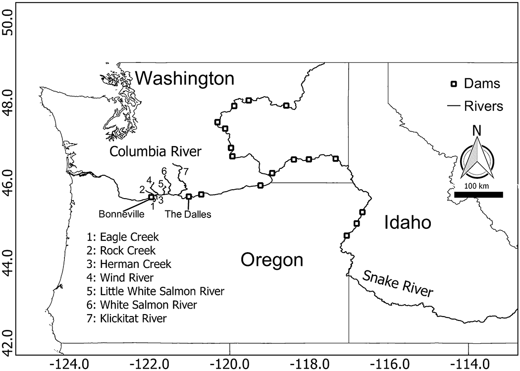
Map of the case study spatial extent (Bonneville dam to The Dalles dam) including significant cold water refuges.

For the case study, we set the area of an individual hexagon to 0.05 ha, with the corresponding diameter (the distance separating parallel edges) being 24.03 m. At this scale, the maps were able to resolve what we considered the smallest usable CWR features. The resulting river complex comprises 162K hexagonal cells representing the Bonneville Reservoir and the tributaries associated with CWRs. Each CWR was made up from a cold water patch in the tributary and the adjacent plume where this water mixed with the Columbia River (Fig. 3).

Fig. 3.

Map of the three model patches: Columbia River, cold water refuge plume, and a cold water refuge tributary, for the Klickitat River, Washington. Cold water refuge plume volume defined by being less than 18 °C.

River temperature data varies by the hour over the 2928 h from July 1 - October 31 (Appendix B). Modeled temperatures were obtained by computing the mean value per Julian day from 2006-2016 for all observations available within each river corridor thermal patch (Fig. 4). That is, a single temperature per hour was estimated for each thermal patch, which in turn consisted of the collection of hexagons representing the mainstem Columbia River (which is well-mixed throughout our study area), each tributary CWR, or each plume CWR. Temperatures assigned to the Bonneville Reservoir (the portion of the mainstem Columbia River falling within our study area) and tributary CWR patches were the mean values observed across multiple temperature loggers. Temperatures within plume areas result from the mixing of tributary and Columbia River flows. We did not have access to observed temperature data from the plumes, so we modeled them using the adjacent tributary and the Bonneville Reservoir temperatures. Appendix B contains a detailed description of this temperature estimation process.

Fig. 4.

Averaged hourly temperature for the tributary portion of seven CWRs and the adjacent Columbia River. Values are mean hourly temperature for each day, across all years for which a site was monitored.

Model parameters

We distinguish the migration corridor simulator input parameters depending on whether their values are well characterized by data (fixed parameters), or if they had to be assigned a value based in part on the emergent model properties they affected (tuning parameters). Examples of fixed parameters include fish initial state data (e.g. mass, CWR residence times), population depth preferences, energy submodel variables, density limits, and mortality rates. These parameters and their associated empirical background are described in more detail in Appendix A. Tuning parameters include the simulated fish movement speeds and their propensity to exhibit specific movement behaviors. As a consequence of this design, the emergent properties characterizing population-scale consequences of interactions between individual fish and their environment were constrained by choice of probabilistic tuning parameters.

The primary emergent model outcomes we evaluated are CWR usage patterns and migration corridor passage timing. The term CWR usage pattern is a reference to an empirical relationship linking river temperature to the proportion of fish residing in CWRs. Passage timing refers to the amount of time individual fish spend traversing the study area. Passage timing and CWR usage are meaningful outcomes for guiding parameter tuning due to their ecological importance, and because empirical observations of these phenomena are available. We found that several tuning parameters affected a single emergent model property.

We tuned our model to fit CWR usage patterns by iteratively adjusting the degree to which temperature and spawn timing influenced fishes’ choice of movement strategy until the simulated CWR usage patterns matched empirical observations derived from Chinook salmon and steelhead tagged in previous studies (Goniea et al. 2006; Keefer et al. 2009). Simulated output and observed data both displayed a large increase in usage of CWR as temperature increased to 19 - 21 °C (Fig. 5). Observed species differences were reflected in model output across the seasonal range of water temperatures, with simulated steelhead exhibiting a higher propensity to hold in CWRs than did the Chinook salmon, consistent with empirical observations.

Fig. 5.

Migration corridor simulation model output showing the percentage of fish residing in cold water refuges for ≥ 4 h in relation to the temperature of the Columbia River on each fish entry date.

Passage timing depends on fish movement speed and behavior, and on CWR usage patterns. We varied hourly movement speeds (values drawn from a distribution and assigned to individuals) until the distribution of simulated fish passage times agreed qualitatively with field data. Our simulated Chinook salmon and steelhead passage times through the Bonneville Reservoir ranged from 2-20 days (mean = 2.3) and 3-80 days (mean = 15.8) respectively, which fit empirical observations (Goniea et al. 2006; Keefer et al. 2009). As entry temperature increased, passage time maximums and medians increased in concert (Fig. 6).

Fig. 6.

Migration corridor simulation model output showing the median, quartile, and range (5-95%) of fall Chinook salmon and summer steelhead passage times through the Bonneville Reservoir in relation to the temperature of the Columbia River on the date each fish entered the reservoir.

We also evaluated overall CWR usage patterns and passage timing by comparing model output to empirical data (Fig. 7 and 8). Reference empirical data were obtained from adult Chinook and steelhead migrants during 2000 and 2002 (Keefer et al. 2018) using intragastric radio data storage transmitters. These tags store depth and internal body temperature, which allow for fine spatial and temporal resolution of their thermal experience. The observed and modelled Chinook salmon thermal time series demonstrate less propensity for CWR residence and shorter duration of CWR use than steelhead thermal histories.

Fig. 7.

Observed and modeled temperature exposure time series for fall Chinook salmon. Individuals were randomly selected from the simulation output to match the number of empirically observed individuals (n=31). Each horizontal line represents an individual fish, panels A and B are organized by the total time each fish spent in the study reach, whereas panel C and D are organized by fish entry date into Bonneville Reservoir. Observed data are summarized from adult Chinook salmon migrants during 2000 with intragastric radio data storage transmitters (Keefer et al. 2018).

Fig. 8.

Observed and modeled temperature exposure time series for summer steelhead. Individuals were randomly selected from the simulation output to match the number of empirically observed individuals (n=69). Each horizontal line represents an individual fish, panels A and B are organized by total time in system, whereas panels C and D are organized by entry date into Bonneville Reservoir. Observed data are summarized from adult steelhead migrants during 2000 with intragastric radio data storage transmitters (Keefer et al. 2018). Radio-tagged fish had a maximum 40-d history, so some of the time series are underestimating passage time.

Assessment Metrics

CWR usage patterns and individual fitness outcomes are the key assessment metrics generated by the migration corridor simulator (Fig. 9 and 10). These model outputs can be used to track fitness within the simulated part of the migration corridor, and have implications for fitness in upstream reaches as well. The migration corridor simulation model quantifies the number of fish in CWRs through time, and the density of fish in each CWR. It can be used to evaluate whether the available capacity and distribution of CWRs along migration corridors limits behavioral thermoregulation of migrating fish and influences fitness outcomes.

Fig. 9.

Migration corridor simulation model output showing (A) total number of fish (Chinook salmon and steelhead) in a refuge through time and (B) effective refuge density through time.

Fig. 10.

Frequency distribution histograms characterizing outcomes from the migration corridor simulation model for the case study showing (A) cumulative degree days, (B) cumulative degree days > 18 °C, (C) energy used during migration (J/g), (D) somatic energy remaining (J/g), (E) date of entry into the Bonneville Reservoir, and (F) date of upstream exit.

Individual fitness outcomes include energy consumption rate and cumulative thermal exposure metrics. In the migration simulation model, energy consumption is primarily determined by thermal exposure, initial mass, and swim speed (Brett 1971; Geist et al. 2003). Fish energy reserves in turn affect spawning success as well as gamete quantity and quality (King et al. 2003; Bowerman et al. 2017). In addition to calculating the energy remaining, the model uses the full post-migration thermal exposure time series to track two cumulative exposure metrics, since these quantities are known to affect spawning success and mortality (Crossin et al. 2008; Bowerman et al. 2017; Connor et al. 2018). The metric titled “accumulated degree days” is the sum of the hourly temperature exposure records for an individual, divided by 24. The metric titled “degree days above 18 °C” is the sum of the hourly temperatures exceeding 18 °C, divided by 24, experienced along each fish’s migration path.

Outcomes

The case study results suggest migration time and fitness cost will vary significantly by individual. To succeed, fish must exit the migration corridor in time to spawn, avoid accumulating degree days above a threshold value, and retain sufficient energy to complete the spawning process. We observed that the simulated fishes’ initial energy density, the migration corridor temperatures they experienced, and their history of behavioral thermoregulation were the primary determinants of their fitness outcomes, and we suggest that our migration corridor simulator can be used to identify migration strategies that optimize these outcomes (Fig. 10). Insights gained from use of the model might be exploited to identify management interventions that encourage beneficial migration strategies and discourage disadvantageous ones. While this pursuit falls outside the scope of the present paper, we hope our work enables and inspires others to perform research of this nature.

Simulated thermal exposure and fitness outcomes reflect observed migration corridor spatio-temporal temperature dynamics and differences in species life histories (Fig. 7 and 8). Steelhead exhibit a higher diversity of migration strategies, and a wider distribution of both migration corridor entry dates and exit dates. Overall, Chinook salmon exit dates from the Bonneville Reservoir are earlier and show less variability when compared to steelhead. Observed shorter passage times for Chinook salmon are an anticipated consequence of their larger mean body size and abbreviated reproductive time table. Simulated steelhead demonstrate higher degree-day accumulations and higher rates of energy consumption (Fig. 10). Spatial patterns of CWR use also reflected species’ differences. Simulations suggest that the Rock Creek and Eagle Creek CWRs are too shallow for extensive use by Chinook salmon, but were used by steelhead individuals from August to mid-September at densities approaching their maximum carrying capacity (Fig. 9).

Excluding harvest, survival rates were nearly 100% for both species in this section of the migration corridor. This was an expected outcome corroborated by other simulation studies (Connor et al. 2018). Energy losses did not approach lethal thresholds (4 KJ/g) because the case study examines a relatively small downstream portion of the Columbia River migration corridor. The energetic costs of behavioral thermoregulation decisions made while traversing the study reach would become manifest weeks to months later, as these individuals passed up to eight additional dams and approached their spawning grounds (Connor et al. 2018; Plumb 2018; University of Washington 2018). The simulated range of energy consumption rate for steelhead is higher than Chinook salmon because of innate size differences between the species. Steelhead enter the migration corridor with a mean mass of 4170 g (+ 1508 se), whereas Chinook salmon average 7900 g (+ 1500 se). Still, significant variation in simulated thermal exposure and net energy expenditure were observed in the Bonneville Reservoir, which would have implications for the survival and reproductive success of fish moving beyond this reach.

Conclusions

This paper describes new methods that extend the suite of tools available to aquatic biologists and conservation practitioners. Specifically, we have illustrated how a 2-dimensional spatially-explicit behavioral and physiological model can be developed and used to simulate fish migration within a river system. Our work complements existing methods, most notably riverine network models (Railsback et al. 2014; Fullerton et al. 2017) and grid-based models (Railsback et al. 2009; Landguth et al. 2016). Advantages of our methodology include: user-definable spatial and temporal scales; the flexibility to allow data availability to dictate model complexity; the ability to work with large river networks and include pools, lakes, estuaries, and other water bodies; the freedom to simulate any number of populations; the ease of linking upland process models or adding terrestrial populations (e.g. bear, beaver); and the availability of HexSim’s broad suite of spatial, demographic, and genetic modeling features (Schumaker and Brookes 2018).

The development of the migration corridor simulation model was motivated by the need to quantify the value of CWRs for fish species migrating up the Columbia River system. For salmon and steelhead populations in lower latitudes migrating through warming river corridors, evidence of ongoing behavioral thermoregulation of populations suggests that the distribution of cold water refuges is critically important (Isaak et al. 2017; Keefer et al. 2018). The case study described here was designed to help researchers explore the disadvantages and advantages of CWR use, and to begin quantifying the potential for management to improve fish fitness outcomes. For example, the migration corridor simulation model could be used to explore how an increase or decrease in the temperature of CWRs might affect fish fitness outcomes. While we developed the simulator for this case study, we intentionally kept it general in order to facilitate its adoption by others. The model is readily transferable to different migration corridors and species. Both the model and case study materials are available from the authors upon request.

Mechanistic simulators developed with the best available data and insights are the most appropriate models for forecasting, as their outputs are defensible and can be expected to remain valid even when environmental conditions and disturbance regimes change. When an ecological system is insufficiently understood to permit the development of a purely mechanistic model, other options are available. Here, we have responded to data limitations by developing a hybrid model that is partly mechanistic and partly probabilistic. We tuned some model parameters to fit empirical data, and as a consequence the model’s emergent outcomes are partially constrained. Nevertheless, data limitations are more the rule than the exception, and in this regard, our model is not unusual. As new data becomes available, our model can be updated incrementally to make it more mechanistic and thus more reliable for forecasting.

For the migration corridor simulation model, the biggest constraint in developing fully mechanistic submodules was a limited understanding of fish movement behavior. Specifically, forecasting ability could be improved with a better understanding of how fish navigate to cold water refuges, how they determine when to leave a refuge, and what key drivers influence individual movement behaviors during refuge stay. The model’s predictive capability could also be improved by including additional studies in the tuning data; the case study incorporated data from a limited number of studies (Goniea et al. 2006; Keefer et al. 2018) and years (1996-2004).

A principal contribution from this work derives from the simulator’s linkage of fish fitness outcomes to migration corridor conditions. The model incorporates changing fine-scale spatio-temporal drivers that directly affect individuals, and then integrates these processes across space and time to resolve population dynamics. Our present goal is to use the model to inquire how altering the distribution and quality of CWRs will influence fish fitness outcomes in the Columbia River system. Future applications of the migration corridor simulator may help identify management strategies, mitigation efforts, and restoration scenarios that better optimize fish viability given the constraints associated with ongoing hydropower operations, land use decisions, and climate change.

Literature Cited

- Arismendi I, Safeeq M, Johnson SL, et al. (2012) Increasing synchrony of high temperature and low flow in western North American streams: double trouble for coldwater biota? Hydrobiologia 712:61–70 [Google Scholar]
- Armstrong JB, Ward EJ, Schindler DE, Lisi PJ (2016) Adaptive capacity at the northern front: sockeye salmon behaviourally thermoregulate during novel exposure to warm temperatures. Conserv Physiol 4:cow039. [DOI] [PMC free article] [PubMed] [Google Scholar]
- August SM, Hicks BJ (2007) Water temperature and upstream migration of glass eels in New Zealand: implications of climate change. Environ Biol Fishes 81:195–205 [Google Scholar]
- Battin J (2004) When Good Animals Love Bad Habitats: Ecological Traps and the Conservation of Animal Populations. Conserv Biol 18:1482–1491 [Google Scholar]
- Bellmore RJ, Duda JJ, Craig LS, et al. (2016) Status and trends of dam removal research in the United States. Wiley Interdisciplinary Reviews: Water 4:e1164 [Google Scholar]
- Berman CH, Quinn TP (1991) Behavioural thermoregulation and homing by spring chinook salmon, Oncorhynchus tshawytscha (Walbaum), in the Yakima River. J Fish Biol 39:301–312 [Google Scholar]
- Bowerman TE, Pinson-Dumm A, Peery CA, Caudill CC (2017) Reproductive energy expenditure and changes in body morphology for a population of Chinook salmon Oncorhynchus tshawytscha with a long distance migration. J Fish Biol 90:1960–1979 [DOI] [PubMed] [Google Scholar]
- Brett JR (1971) Energetic Responses of Salmon to Temperature. A Study of Some Thermal Relations in the Physiology and Freshwater Ecology of Sockeye Salmon (Oncorhynchus nerkd). Am Zool 11:99–113 [Google Scholar]
- Busby PJ, Wainwright TC, Bryant GJ, et al. (1996) Status Review of West Coast Steelhead from Washington, Idaho, Oregon, and California. U.S. Department of Commerce, National Marine Fisheries Service, Northwest Fisheries Science Center [Google Scholar]
- Connor WP, Tiffan KF, Chandler JA, et al. (2018) Upstream Migration and Spawning Success of Chinook Salmon in a Highly Developed, Seasonally Warm River System. Reviews in Fisheries Science & Aquaculture; 1–50 [Google Scholar]
- Cooke SJ, Hinch SG, Farrell AP, et al. (2008) Developing a mechanistic understanding of fish migrations by linking telemetry with physiology, behavior, genomics and experimental biology: an interdisciplinary case study on adult Fraser River sockeye salmon. Fisheries 33:321–339 [Google Scholar]
- Crossin GT, Hinch SG, Cooke SJ, et al. (2008) Exposure to high temperature influences the behaviour, physiology, and survival of sockeye salmon during spawning migration. Can J Zool 86:127–140 [Google Scholar]
- Crossin GT, Hinch SG, Farrell AP, et al. (2004) Energetics and morphology of sockeye salmon: effects of upriver migratory distance and elevation. J Fish Biol 65:788–810 [Google Scholar]
- Crozier LG, Bowerman TE, Burke BJ, et al. (2017) High-stakes steeplechase: a behavior-based model to predict individual travel times through diverse migration segments. Ecosphere 8:e01965 [Google Scholar]
- Deslauriers D, Chipps SR, Breck JE, et al. (2017) Fish Bioenergetics 4.0: An R-Based Modeling Application. Fisheries 42:586–596 [Google Scholar]
- Dickerson BR, Brinck KW, Willson MF, et al. (2005) Relative importance of salmon body size and arrival time at breeding grounds to reproductive success. Ecology 86:347–352 [Google Scholar]
- Dietrich JP, Van Gaest AL, Strickland SA, Arkoosh MR (2014) The impact of temperature stress and pesticide exposure on mortality and disease susceptibility of endangered Pacific salmon. Chemosphere 108:353–359 [DOI] [PubMed] [Google Scholar]
- Dunning JB, Danielson BJ, Ronald Pulliam H (1992) Ecological Processes That Affect Populations in Complex Landscapes. Oikos 65:169 [Google Scholar]
- Ebersole JL, Liss WJ, Frissell CA (2001) Relationship between stream temperature, thermal refugia and rainbow trout Oncorhynchus mykiss abundance in arid-land streams in the northwestern United States. Ecol Freshw Fish 10:1–10 [Google Scholar]
- Fausch KD, Torgersen CE, Baxter CV, Li HW (2002) Landscapes to Riverscapes: Bridging the Gap between Research and Conservation of Stream Fishes. Bioscience 52:483 [Google Scholar]
- Frissell CA, Liss WJ, Warren CE, Hurley MD (1986) A hierarchical framework for stream habitat classification: Viewing streams in a watershed context. Environ Manage 10:199–214 [Google Scholar]
- Fullerton AH, Burke BJ, Lawler JJ, et al. (2017) Simulated juvenile salmon growth and phenology respond to altered thermal regimes and stream network shape. Ecosphere 8:1–23 [DOI] [PMC free article] [PubMed] [Google Scholar]
- Geist DR, Brown RS, Cullinan VI, et al. (2003) Relationships between metabolic rate, muscle electromyograms and swim performance of adult chinook salmon. J Fish Biol 63:970–989 [Google Scholar]
- Goniea TM, Keefer ML, Bjornn TC, et al. (2006) Behavioral Thermoregulation and Slowed Migration by Adult Fall Chinook Salmon in Response to High Columbia River Water Temperatures. Trans Am Fish Soc 135:408–419 [Google Scholar]
- Healey M (2011) The cumulative impacts of climate change on Fraser River sockeye salmon (Oncorhynchus nerka) and implications for management. Can J Fish Aquat Sci 68:718–737 [Google Scholar]
- Isaak DJ, Wenger SJ, Young MK (2017) Big biology meets microclimatology: defining thermal niches of ectotherms at landscape scales for conservation planning. Ecol Appl 27:977–990 [DOI] [PubMed] [Google Scholar]
- Isaak DJ, Wollrab S, Horan D, Chandler G (2011) Climate change effects on stream and river temperatures across the northwest U.S. from 1980–2009 and implications for salmonid fishes. Clim Change 113:499–524 [Google Scholar]
- Isaak DJ, Young MK, Luce CH, et al. (2016) Slow climate velocities of mountain streams portend their role as refugia for cold-water biodiversity. Proc Natl Acad Sci U S A 113:4374–4379 [DOI] [PMC free article] [PubMed] [Google Scholar]
- Jager HI, DeAngelis DL (2018) The confluences of ideas leading to, and the flow of ideas emerging from, individual-based modeling of riverine fishes. Ecol Modell 384:341–352 [Google Scholar]
- Jepson MA, Keefer ML, Naughton GP, et al. (2010) Population Composition, Migration Timing, and Harvest of Columbia River Chinook Salmon in Late Summer and Fall. N Am J Fish Manage 30:72–88 [Google Scholar]
- Jonsson B, Jonsson N (2009a) A review of the likely effects of climate change on anadromous Atlantic salmon Salmo salar and brown trout Salmo trutta, with particular reference to water temperature and flow. J Fish Biol 75:2381–2447 [DOI] [PubMed] [Google Scholar]
- Jonsson B, Jonsson N (2009b) Migratory timing, marine survival and growth of anadromous brown troutSalmo truttain the River Imsa, Norway. J Fish Biol 74:621–638 [DOI] [PubMed] [Google Scholar]
- Keefer ML, Clabough TS, Jepson MA, et al. (2018) Thermal exposure of adult Chinook salmon and steelhead: Diverse behavioral strategies in a large and warming river system. PLoS One 13:e0204274. [DOI] [PMC free article] [PubMed] [Google Scholar]
- Keefer ML, Peery CA, High B (2009) Behavioral thermoregulation and associated mortality trade-offs in migrating adult steelhead (Oncorhynchus mykiss): variability among sympatric populations. Can J Fish Aquat Sci 66:1734–1747 [Google Scholar]
- Keefer ML, Peery CA, Jepson MA, Stuehrenberg LC (2004) Upstream migration rates of radio-tagged adult Chinook salmon in riverine habitats of the Columbia River basin. J Fish Biol 65:1126–1141 [Google Scholar]
- King HR, Pankhurst NW, Watts M, Pankhurst PM (2003) Effect of elevated summer temperatures on gonadal steroid production, vitellogenesis and egg quality in female Atlantic salmon. J Fish Biol 63:153–167 [Google Scholar]
- Klemetsen A, Amundsen P-A, Dempson JB, et al. (2003) Atlantic salmon Salmo salar L., brown trout Salmo trutta L. and Arctic charr Salvelinus alpinus (L.): a review of aspects of their life histories. Ecol Freshw Fish 12:1–59 [Google Scholar]
- Landguth EL, Bearlin A, Day CC, Dunham J (2016) CDMetaPOP: an individual-based, eco-evolutionary model for spatially explicit simulation of landscape demogenetics. Methods Ecol Evol 8:4–11 [Google Scholar]
- Lassalle G, Rochard E (2009) Impact of twenty-first century climate change on diadromous fish spread over Europe, North Africa and the Middle East. Glob Chang Biol 15:1072–1089 [Google Scholar]
- Lennox RJ, Chapman JM, Souliere CM, et al. (2016) Conservation physiology of animal migration. Conserv Physiol 4:cov072. [DOI] [PMC free article] [PubMed] [Google Scholar]
- McCullough DA, Bartholow JM, Jager HI, et al. (2009) Research in Thermal Biology: Burning Questions for Coldwater Stream Fishes. Rev Fish Sci 17:90–115 [Google Scholar]
- Mesa MG, Magie CD (2006) Evaluation of energy expenditure in adult spring Chinook salmon migrating upstream in the Columbia River Basin: an assessment based on sequential proximate analysis. River Res Appl 22:1085–1095 [Google Scholar]
- Montgomery D (2003) King of Fish: The Thousand-Year Run of Salmon. Basic Books [Google Scholar]
- Ohlberger J, Ward EJ, Schindler DE, Lewis B (2018) Demographic changes in Chinook salmon across the Northeast Pacific Ocean. Fish Fish 19:533–546 [Google Scholar]
- Penaluna BE, Dunham JB, Railsback SF, et al. (2015) Local Variability Mediates Vulnerability of Trout Populations to Land Use and Climate Change. PLoS One 10:e0135334. [DOI] [PMC free article] [PubMed] [Google Scholar]
- Pickering AD, Pottinger TG (1989) Stress responses and disease resistance in salmonid fish: Effects of chronic elevation of plasma cortisol. Fish Physiol Biochem 7:253–258 [DOI] [PubMed] [Google Scholar]
- Plumb JM (2018) A bioenergetics evaluation of temperature-dependent selection for the spawning phenology by Snake River fall Chinook salmon. Ecol Evol. doi: 10.1002/ece3.4353 [DOI] [PMC free article] [PubMed] [Google Scholar]
- Poole GC (2002) Fluvial landscape ecology: addressing uniqueness within the river discontinuum. Freshw Biol 47:641–660 [Google Scholar]
- Quinn TP (2011) The Behavior and Ecology of Pacific Salmon and Trout. UBC Press [Google Scholar]
- Railsback SF, Harvey BC, Jackson SK, Lamberson RH (2009) InSTREAM: the individual-based stream trout research and environmental assessment model [Google Scholar]
- Railsback SF, Harvey BC, White JL (2014) Facultative anadromy in salmonids: linking habitat, individual life history decisions, and population-level consequences. Can J Fish Aquat Sci 71:1270–1278 [Google Scholar]
- Richter A, Kolmes SA (2005) Maximum Temperature Limits for Chinook, Coho, and Chum Salmon, and Steelhead Trout in the Pacific Northwest. Rev Fish Sci 13:23–49 [Google Scholar]
- Robards MD, Quinn TP (2002) The Migratory Timing of Adult Summer-Run Steelhead in the Columbia River over Six Decades of Environmental Change. Trans Am Fish Soc 131:523–536 [Google Scholar]
- Roscoe DW, Hinch SG, Cooke SJ, Patterson DA (2010) Behaviour and thermal experience of adult sockeye salmon migrating through stratified lakes near spawning grounds: the roles of reproductive and energetic states. Ecol Freshw Fish 19:51–62 [Google Scholar]
- Schaffer WM, Elson PF (1975) The Adaptive Significance of Variations in Life History among Local Populations of Atlantic Salmon in North America. Ecology 56:577–590 [Google Scholar]
- Schlosser IJ (1995) Critical landscape attributes that influence fish population dynamics in headwater streams. Hydrobiologia 303:71–81 [Google Scholar]
- Schumaker NH, Brookes A (2018) HexSim: a modeling environment for ecology and conservation. Landsc Ecol 33:197–211 [DOI] [PMC free article] [PubMed] [Google Scholar]
- Silva AT, Lucas MC, Castro-Santos T, et al. (2017) The future of fish passage science, engineering, and practice. Fish Fish 19:340–362 [Google Scholar]
- Stewart DJ, Ibarra M (1991) Predation and Production by Salmonine Fishes in Lake Michigan, 1978–88. Can J Fish Aquat Sci 48:909–922 [Google Scholar]
- Strange JS (2012) Migration Strategies of Adult Chinook Salmon Runs in Response to Diverse Environmental Conditions in the Klamath River Basin. Trans Am Fish Soc 141:1622–1636 [Google Scholar]
- Taranger GL, Hansen T (1993) Ovulation and egg survival following exposure of Atlantic salmon, Salmo salar L., broodstock to different water temperatures. Aquac Res 24:151–156 [Google Scholar]
- Torgersen CE, Ebersole JL, Keenan ADM (2012) Primer for identifying cold-water refuges to protect and restore thermal diversity in riverine landscapes. U.S. Environmental Protection Agency [Google Scholar]
- Torgersen CE, Price DM, Li HW, McIntosh BA (1999) Multiscale Thermal Refugia and Stream Habitat Associations of Chinook Salmon in Northeastern Oregon. Ecol Appl 9:301 [Google Scholar]
- University of Washington (2018) fish passage data. In: Columbia River DART (Data Access Real Time). https://www.cbr.washington.edu/dart. Accessed 27 Nov 2018
- Vannote RL, Wayne Minshall G, Cummins KW, et al. (1980) The River Continuum Concept. Can J Fish Aquat Sci 37:130–137 [Google Scholar]
- Waknitz WF, Matthews GM, Wainwright T, Winans GA (1995) Status Review for Mid-Columbia River Summer Chinook Salmon. US Department of Commerce, National Oceanic and Atmoospheric Administration, National Marine Fisheries Service, Northwest Fisheries Science Center. [Google Scholar]
- Walter RP, Hogan JD, Blum MJ, et al. (2012) Climate change and conservation of endemic amphidromous fishes in Hawaiian streams. Endanger Species Res 16:261–272 [Google Scholar]
- Waples RS, Zabel RW, Scheuerell MD, Sanderson BL (2008) Evolutionary responses by native species to major anthropogenic changes to their ecosystems: Pacific salmon in the Columbia River hydropower system. Mol Ecol 17:84–96 [DOI] [PubMed] [Google Scholar]
- Wu H, Kimball JS, Elsner MM, et al. (2012) Projected climate change impacts on the hydrology and temperature of Pacific Northwest rivers. Water Resour Res 48.: doi: 10.1029/2012wr012082 [DOI] [Google Scholar]
Associated Data
This section collects any data citations, data availability statements, or supplementary materials included in this article.