A SIQ mathematical model on COVID-19 investigating the lockdown effect

Abstract

This research paper aims at studying the impact of lockdown on the dynamics of novel Corona Virus Disease (COVID-19) emerged in Wuhan city of China in December 2019. Perceiving the pandemic situation throughout the world, Government of India restricted international passenger traffic through land check post (Liang, 2020) and imposed complete lockdown in the country on 24 March 2020. To study the impact of lockdown on disease dynamics we consider a three-dimensional mathematical model using nonlinear ordinary differential equations. The proposed model has been studied using stability theory of nonlinear ordinary differential equations. Basic reproduction ratio is computed and significant parameters responsible to keep basic reproduction ratio less than one are identified. The study reveals that disease vanishes from the system only if complete lockdown is imposed otherwise disease will always persist in the population. However, disease can be kept under control by implementing contact tracing and quarantine measures as well along with lockdown if lockdown is imposed partially.

1. Introduction

The novel Corona Virus Disease (COVID-19) was first manifested in Wuhan, China in late 2019 that has travelled across different countries and spread at quite a fast pace by human to human infection (Bhola et al., 2020; Binti et al., 2020; Li et al., 2020). Within a very short span of time the disease has spread in major part of the world leading to large number of deaths. Migration of individuals from China to other parts of world played a critical role in the spread of infectious disease COVID-19. China could control the disease by introducing lockdown in Wuhan since, it was only option available due to the absence of targeted drug and vaccine against the virus. This pandemic led the Government of India to impose complete lockdown in the country on March 24, 2020 and is still in lockdown stage as of May 17, 2020. Literatures report that lockdown measure is significant because it has been able to reduce the transmission of COVID-19 by as much as 84 percent as in France (Barnett & Walker, 2008). Principle feature of lockdown is reduction of immigration of population to nearly zero. It is quite evident from the past that immigration of population plays a significant role in the spread of infectious diseases like flu. It has been reported that immigration has not only played roles in introducing infections into native populations but also in changing the incidence of infections, and in increasing the prospects of local transmission (Spiteri et al., 2020). Immigration of infective population from COVID-19 region has posed risk to the local population and increased the geographic range of the disease at such a fast pace that it spread in 28 countries by 21 February 2020 (Eunha, 2006). This article focuses on the impact of lockdown as preventive measure through mathematical modeling approach. Modeling the effect of lockdown to prevent the spread of disease is a complex task however we have modelled it by introducing the immigration term in the model and comparing it with the model without immigration term. Contact tracing, immigration of individual has been taken as one of the most important features in studying the disease dynamics by some of the mathematical modellers given in (Day et al., 2006; Kwok et al., 2019; Ndairou et al., 2020; Wang, 2004; Wang & Zhao, 2006; Yang et al., 2009). We have introduced immigration of susceptible individuals along with a fraction of infective individuals directly in the infective compartment and compared it with the model without immigration. In addition, we have also considered contact tracing and quarantine as other preventive measures in our mathematical model. Quarantine is one of the live options during disease outbreaks. Fraser et al. in (Fraser et al., 2004), shows that the quarantine is an effective measure if asymptomatic infection are responsible for a large number of infections as seen in COVID-19 cases. The author further concluded in his study on SARS that its outbreak could be controlled effectively by sufficient isolation of symptomatic individuals. On the other hand, Chen et al. (Chen et al., 2006) reported that even with less efficient contact tracing an outbreak of SARS with effective isolation of symptomatic patients is sufficient to control SARS outbreak. Thus, objective of this paper is to study the combined effect of lockdown, contact tracing and quarantine on the COVID-19 dynamics. These measures are important since there is no specific antiviral treatment up to date hence prevention is the only way to keep the disease under control. Mathematical modeling can help by evaluating the effectiveness of these preventive measures in the early phase of epidemics of new emerging outbreak in the future (Jia et al., 2020).

To the best of our knowledge combined effect of all these measures, lockdown, contact tracing and quarantine has not been considered in any of the previous mathematical model on COVID-19. Our research paper is organised as follows: In section 2 mathematical model is discussed, section 3 represents boundedness of the system. In section 4 model dynamics without lockdown effect is studied followed by section 5 manifesting the lockdown effect in the system. In section 6, numerical analysis is performed and paper is concluded in result and discussion section 7.

2. Mathematical model

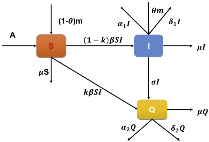
We consider a three-dimensional model with susceptible population S(t), infective population I(t) and quarantined population Q(t). It is assumed that the population is homogeneously mixed and disease spreads via the direct contact between susceptible and infective individuals as well by immigration of individuals in susceptible class and in infective class. Thus, we have an SIQ model with immigration. Let N(t) be the total population at any time t in the region under consideration, which is the sum of three subpopulation. Susceptible population is entering in the system at the constant rate A and by immigration (1 −θ)m. Whereas fraction θm is entering directly to the infective class with the assumption that a fraction of immigrants are infective are carrier of virus. We have studied the impact of lockdown in the model by taking immigration term as zero because immigration is restricted to a large extent during lockdown period. Moreover, by contact tracing, some of the infective individuals are quarantined and only fraction of the infective’s are entering into the class of infective and spreading infection among the susceptible. We model here the average effect of contact-tracing based strategy (Aparicio & Hernandez, 2006). Let k be the rate of contact tracing of individuals so that a fraction (1 − k) are responsible for spreading infection and rest are quarantined. We have assumed Holling type-II functional response to model the interaction between susceptible and infective populations, where α and η are the infection catching and handling time of the virus from the infective individual to the susceptible individuals. μ is the natural mortality rate of population in each compartment, δ₁ and δ₂ are the recovery rate of the infective and quarantined population whereas α₁ and α₂ are the disease related death rates of the infective and quarantined compartments respectively. Infected individuals are assumed to be quarantined at the rate σ. Thus, with these assumptions we have formulated a three dimensional epidemiological model taking susceptible S(t), infective I(t) and quarantined Q(t) population as system variables. A schematic flow diagram is represented in Fig. 1 to understand the dynamics of COVID-19.

Fig. 1.

Schematic flow diagram of the SIQ COVID-19 model.

The model equations with immigration are given by

$$\frac{dS}{dt}=A-\frac{\beta SI}{\alpha +\eta I}-\mu S+(1-\theta )m,$$ (1)

$$\frac{dI}{dt}=\frac{(1-k)\beta SI}{\alpha +\eta I}-\mu I-{\delta }_{1}I-\sigma I-{\alpha }_{1}I+\theta m,$$ (2)

$$\frac{dQ}{dt}=\frac{k\beta SI}{\alpha +\eta I}+\sigma I-\mu Q-{\delta }_{2}Q-{\alpha }_{2}Q,$$ (3)

with initial conditions S(0) > 0, I(0) ≥ 0 Q(0) ≥ 0.

Description of parameters is defined in Table 1.

Table 1.

Description of parameters.

Parameter	Description
A	recruitment rate
α	half saturation constant
η	positive constant
β	transmission rate of infection
μ	natural death rate
m	number of migrants
θ	rate of infected migrants
k	rate of contact tracing
δ1	rate of recovery of infective population
δ2	rate of recovery of quarantined population
σ	transition rate from infective to quarantined population
α1	disease related death rate of infective population
α2	disease related death rate of quarantined population

3. Boundedness of the system

In the following lemma, we state the bounds of system variables which is further used to prove the analytic results. Boundedness of the system may be interpreted as a natural restriction to indefinite growth of infective population because of various constraints either due to natural conditions or due to preventive habits acquired by the population to keep themselves safe from the disease. We will show that the solutions of system are bounded to ensure the biological validity of the model.

Lemma 1

The set $\Omega =\left\{(S,I,Q):0\le N=S+I+Q\le N_m\right\}$ is the region of attraction for all solutions initiating in the interior of the positive octant, where $N_m=\frac{A+m}{\mu }$.

Proof Let (S, I, Q) be the solution with positive initial values (S₀, I₀, Q₀). From system of equations , we get

$$\frac{dN}{dt}=A-\mu N+m-({\delta }_1+{\alpha }_1)I-({\delta }_2+{\alpha }_2)Q,$$

$$\frac{dN}{dt}\le A-\mu N+m.$$

According to comparison principle, it follows that $N_m=\frac{A+m}{\mu }$. This completes the Proof.

4. Model dynamics without lockdown effect

When m≠0 then the model (1)–(3) has no disease-free equilibrium point, only pandemic equilibrium exists. Thus, when immigration of population is allowed in the system and a fraction of them are infective; disease cannot be vanished to zero, although attempts may be made to control the disease.

4.1. Equilibrium analysis

In a dynamical system an equilibrium point is a state of the system that does not change with time. Thus, if the system starts at an equilibrium point, the state will remain at the equilibrium forever. We are interested in finding the equilibrium state of system when it is free from disease that is, disease free equilibrium point and the equilibrium state of persistence of disease, the endemic/pandemic equilibrium point. For the system of equations (1), (2), (3), only pandemic equilibrium E^m(S^m, I^m, Q^m) exists. The values of S^m, I^m and Q^m for the pandemic equilibrium are $S^m=\frac{A+(1-\theta )m(\alpha +\eta I^m)}{\mu \alpha +(\beta +\mu \eta )I^m},Q^m=\frac{k\beta (A+(1-\theta )m)I^m}{(\mu +{\delta }_2+{\alpha }_2)(\mu \alpha +(\beta +\mu \eta )I^m)}+\frac{\sigma I^m}{(\mu +{\delta }_2+{\alpha }_2)}\text{and}{I}^m$ is the root of the quadratic equation (4) with $R_0=\frac{(1-k)\beta A}{\alpha \mu (\mu +{\delta }_1+\sigma +{\alpha }_1)}$

$${(I^m)}^2-\left(\frac{\theta m}{\mu +{\delta }_1+\sigma +{\alpha }_1}+\frac{(R_0-1)\mu \alpha }{(\beta +\mu \eta )}\right)I^m-\frac{\mu \alpha \theta m}{\mu +{\delta }_1+\sigma +{\alpha }_1}=0,$$ (4)

which guarantees that unique positive equilibrium point E^m exist iff R₀ > 1.

4.2. Local stability analysis of pandemic equilibrium point

Local stability analysis of equilibrium points gives an insight into the impact of small perturbations in the equilibrium state of the system. To study the stability of pandemic equilibrium point, we linearize the system about the arbitrary equilibrium points E^m(S^m, I^m, Q^m) and obtain the corresponding Jacobian matrix as given by

$$J_{E^m}=\left[\begin{array}{ccc}{b}_{11}& b_{12}& 0\\ b_{21}& b_{22}& 0\\ b_{31}& b_{32}& b_{33}\end{array}\right],$$

where $b_{11}=-\frac{\beta I^m}{(\alpha +\eta I^m)}-\mu ,b_{12}=-\frac{\alpha \beta S^m}{{(\alpha +\eta I^m)}^2},b_{21}=\frac{(1-k)\beta I^m}{\alpha +\eta I^m},b_{22}=\frac{\alpha (1-k)\beta S^m}{{(\alpha +\eta I^m)}^2}-\mu -{\delta }_1-\sigma -{\alpha }_1,b_{31}=\frac{k\beta I^m}{\alpha +\eta I^m},b_{32}=\frac{\alpha k\beta S^m}{{(\alpha +\eta I^m)}^2}+\sigma ,b_{33}=-\mu -{\delta }_2-{\alpha }_2$.

Proposition

Equilibrium point E^m(S^m, I^m, Q^m) of the system (1)-(3) is locally asymptotically stable if (b₁₁ + b₂₂ < 0).

Proof: From the Jacobean matrix $J_{E^m}$ we observe that the eigenvalues of E^m(S^m, I^m, Q^m) are given by λ₁ = −(μ + δ₂ + α₂) < 0 and other two eigenvalues λ₂ and λ₂ are the roots of the quadratic equation

$${\lambda }^2-(b_{11}+b_{22})\lambda +(b_{11}{b}_{22}-b_{12}{b}_{21})=0.$$

$${\lambda }_{2,3}=\frac{(b_{11}+b_{22})\pm \sqrt{{(b_{11}-b_{22})}^2+4(b_{12}{b}_{21})}}{2}.$$

Thus, the equilibrium E^m will be locally asymptotically stable if (b₁₁ + b₂₂) < 0, which is obvious from the expression of b₁₁ and b₂₂. Since both of them are negative if and only if pandemic equilibrium state of infective population is positive and equation (4) states that infective population is positive if and only if R₀ > 1. Thus, we may conclude that the pandemic equilibrium point is locally asymptotically stable if R₀ > 1. Biologically it may be interpreted by the statement that the system will return back to the pandemic equilibrium point and stays close to it when number of secondary infections produced by a single infective during his complete infectious period is more than one.

4.3. Persistence of the model

Here in this section we found persistence of the disease. The word ‘Persistence’ stands for the survival of each population in future time. We study persistence of the system to determine the conditions under which a disease persists in the system. Persistence of the model (1)–(3) is proved using the following Lemma.

Lemma 2

Assume that $(\mu +{\delta }_1+\sigma +{\alpha }_1)>\frac{(1-k)\beta S_{min}}{(\alpha +\eta N_m)}$, here N_m is upper bound of the populations S, I, Q respectively are always positive; the system of equations (1), (2), (3) persists.

Proof From first equation (1), we have

$$\frac{dS}{dt}\ge A+(1-\theta )m-(\beta N_m+\mu )S,$$

using boundedness and comparison principle, we have

$$S_{min}=\frac{A+(1-\theta )m}{\beta N_m+\mu },$$

S_min is always positive. From equation (2), we have

$$\frac{dI}{dt}\ge \frac{(1-k)\beta S_{min}I}{\alpha +\eta N_m}-(\mu +{\delta }_1+\sigma +{\alpha }_1)I+\theta m,$$

$$\frac{dI}{dt}\ge \theta m-\left\{(\mu +{\delta }_1+\sigma +{\alpha }_1)-\frac{(1-k)\beta S_{min}}{\alpha +\eta N_m}\right\}I,$$

Again, using system boundedness and comparison principle

$$I_{min}=\frac{\theta m}{(\mu +{\delta }_1+\sigma +{\alpha }_1)-\frac{(1-k)\beta S_{min}}{\alpha +\eta N_m}},$$

with condition $(\mu +{\delta }_1+\sigma +{\alpha }_1)>\frac{(1-k)\beta S_{min}}{\alpha +\eta N_m}$. I_min always remains positive. From the last equation (3) of the system, we get

$$\frac{dQ}{dt}\ge \frac{k\beta S_{min}{I}_{min}}{\alpha +\eta N_m}+\sigma I_{min}-(\mu +{\delta }_2+{\alpha }_2)Q,$$

Again using the comparison principle,

$$Q_{min}=\frac{\frac{k\beta S_{min}{I}_{min}}{\alpha +\eta N_m}+\sigma I_{min}}{(\mu +{\delta }_2+{\alpha }_2)},$$

Q_min remains always positive. This completes the proof of the Lemma.

5. Model dynamics with lockdown effect

To study the impact of lockdown effect, we study the model (1)–(3) for m = 0, that is when immigration of the population in the system is strictly prohibited.

In this case, the model reduces to the following system of equations (5), (6), (7)

$$\frac{dS}{dt}=A-\frac{\beta SI}{\alpha +\eta I}-\mu S,$$ (5)

$$\frac{dI}{dt}=\frac{(1-k)\beta SI}{\alpha +\eta I}-\mu I-{\delta }_{1}I-\sigma I-{\alpha }_{1}I,$$ (6)

$$\frac{dQ}{dt}=\frac{k\beta SI}{\alpha +\eta I}+\sigma I-\mu Q-{\delta }_{2}Q-{\alpha }_{2}Q,$$ (7)

with initial conditions S(0) > 0, I(0) ≥ 0 and Q(0) ≥ 0.

5.1. Basic reproduction number

Basic Reproduction Number (Brauer & Castillo, 2001; Chavez et al., 2002; Driessche & Watmough, 2002; Nyabadza & Hove-Musekwa, 2010) is a threshold number that determines number of secondary infections produced by an infective individual during his or her whole infectious period in a population in which every individual is susceptible. We determine basic reproduction number using next generation matrix approach (Driessche & Watmough, 2002). The decomposition of the model into components R₁ and R₂ leads to system (5)-(7)of the form

$$X=R_1-R_2,$$

where

$$R_1=\left[\begin{array}{c}\frac{(1-k)\beta SI}{\alpha +\eta I}\\ \frac{k\beta SI}{\alpha +\eta I}\\ 0\end{array}\right],$$

$$R_2=\left[\begin{array}{c}\mu I+{\delta }_{1}I+\sigma I+{\alpha }_{1}I\\ \mu Q+{\delta }_{2}Q+{\alpha }_{2}Q-\sigma I\\ \mu S-A\end{array}\right]$$

and

$$X=\left[\begin{array}{c}\frac{dI}{dt},\frac{dQ}{dt},\frac{dS}{dt}\end{array}\right].$$

Since, the infected compartments are I and Q, at the disease free equilibrium point, we define

$$\widetilde{R_1}=\left[\frac{\partial {(R_1)}_i}{\partial x_j}\right],$$

and

$$\widetilde{R_2}=\left[\frac{\partial {(R_2)}_i}{\partial x_j}\right]$$

for 1 ≤ i, j ≤ 2.

$$\widetilde{R_1}=\left[\begin{array}{cc}\frac{(1-k)\beta A}{\alpha \mu }& 0\\ \frac{k\beta A}{\alpha \mu }& 0\end{array}\right],$$

$$\widetilde{R_2}=\left[\begin{array}{c}\mu +{\delta }_1+\sigma +{\alpha }_{1}0-\sigma \\ & \mu +{\delta }_2+{\alpha }_2\end{array}\right].$$

Note that, $\widetilde{R_1}$ is non negative and $\widetilde{R_2}$ is a non singular matrix with ${\widetilde{R_2}}^{-1}$ as non-negative and $\widetilde{R_1}{\widetilde{R_2}}^{-1}$ as non negative matrix; $\widetilde{R_1}{\widetilde{R_2}}^{-1}$ is the next generation matrix. In this case if

$$\begin{array}{ccc}\widetilde{R_1}{\widetilde{R_2}}^{-1}& =\left[\begin{array}{cc}\frac{(1-k)\beta A}{\alpha \mu }& 0\\ \frac{k\beta A}{\alpha \mu }& 0\end{array}\right]\frac{1}{(\mu +{\delta }_2+{\alpha }_2)}\frac{1}{(\mu +{\delta }_1+\sigma +{\alpha }_1)}\left[\begin{array}{c}\mu +{\delta }_2+{\alpha }_{2}0-\sigma \\ & \mu +{\delta }_1+\sigma +{\alpha }_1\end{array}\right],& \\ & =\frac{1}{(\mu +{\delta }_2+{\alpha }_2)(\mu +{\delta }_1+\sigma +{\alpha }_1)}\left[\begin{array}{cc}\mu +{\delta }_2+{\alpha }_2(1-k)\beta A& 0\\ \frac{k\beta A(\mu +{\delta }_2+{\alpha }_2)}{\alpha \mu }& 0\end{array}\right]& \end{array}$$

then the spectral eigenvalue of matrix is $\lambda =\frac{(1-k)\beta A}{\alpha \mu (\mu +{\delta }_1+\sigma +{\alpha }_1)}$. Hence, Basic reproduction number is given by

$$R_0=\frac{(1-k)\beta A}{\alpha \mu (\mu +{\delta }_1+\sigma +{\alpha }_1)}.$$

From the mathematical expression of basic reproduction ratio we observe that it is directly proportional to the susceptible population at disease free state $\frac{A}{\mu }$, infectious period $\frac{1}{(\mu +{\delta }_1+\sigma +{\alpha }_1)}$ and transmission rate of infection β. Along with these terms it is inversely proportional to rate of contact tracing k and half saturation constant α. Thus, spread of disease can be controlled by keeping a check on these parameter values.

5.2. Sensitivity analysis of basic reproduction number R₀

Based on each of the parameters of R₀, sensitivity analysis is performed to check the sensitivity of the basic reproduction number (Arriola & Hyman, 2003; Koonprasert & Chananngam, 2017). In order to reduce the effect of corona virus, it is necessary to control the parameter values to make R₀ < 1. We are therefore interested in finding the rate of change of R₀ as the parameter values are changed. The rate of change of R₀ for a change in value of parameter h can be estimated from $SI[h]=\frac{h}{R_0}\times \frac{\partial R_0}{\partial h}$. The normalized sensitivity indices of the reproduction number with respect to parameter k, α, μ, δ₁, σ, α₁ are given by

$$SI[k]=-\frac{k}{(1-k)}<1,$$

$$SI[\alpha ]=-1<1,$$

$$SI[{\delta }_1]=-\frac{{\delta }_1}{(\mu +{\delta }_1+\sigma +{\alpha }_1)}<1,$$

$$SI[\sigma ]=-\frac{\sigma }{(\mu +{\delta }_1+\sigma +{\alpha }_1)}<1,$$

$$SI[{\alpha }_1]=-\frac{{\alpha }_1}{(\mu +{\delta }_1+\sigma +{\alpha }_1)}<1,$$

$$SI[\beta ]=1,$$

$$SI[\mu ]=-1-\frac{\mu }{(\mu +{\delta }_1+\sigma +{\alpha }_1)}<1,$$

from the above calculations it is obvious that R₀ is mainly sensitive to alters in β. The value of R₀ will be enhanced if we raise the value of β and rest of indices are negative i.e., the value of R₀ decreases as k, α, δ₁, σ, α₁ and μ increase. Thus, basic reproduction number increases proportionally with the increase in rate of transmission of infection and decreases with the rate of contact tracing, half saturation constant, recovery rate of infective population, rate of transition from infective to quarantined population, disease related death rate of infective population and natural death rate of each population.

5.3. Equilibrium analysis of the steady states and stability of equilibriums

System (5)–(7) has two equilibrium points, one is the Disease free equilibrium point and another is pandemic equilibrium point.

Theorem

The SIQ model (5)-(7) has a unique Disease free equilibrium $E_0\left(\frac{A}{\mu },0,0\right)$ for all parameter values. As well as the system under consideration has also a unique pandemic equilibrium $\widehat{E}(\widehat{S},\widehat{I},\widehat{Q})$ under the condition R₀ > 1.

Proof: Pandemic equilibrium point is given by $\widehat{E}(\widehat{S},\widehat{I},\widehat{Q})$, using equations (5), (7) we have $\widehat{S}=\frac{A(\alpha +\eta \widehat{I})}{\mu \alpha +(\beta +\mu \eta )\widehat{I}}$, and $\widehat{Q}=\frac{\beta A\widehat{I}}{(\mu +{\delta }_2+{\alpha }_2)[\mu \alpha +(\beta +\mu \eta )\widehat{I}]}+\frac{\sigma \widehat{I}}{\mu +{\delta }_2+{\alpha }_2}$ respectively. Next putting the value of $\widehat{S}$ in equation (6), we get ${\widehat{I}}^2-\frac{(R_0-1)\mu \alpha \widehat{I}}{\beta +\mu \eta }=0$. From above equation, we get $\widehat{I}=0\text{or}\widehat{I}=\frac{(R_0-1)\mu \alpha }{\beta +\mu \eta }$. The equilibrium $\widehat{E}$ exists if R₀ > 1.

5.4. Local stability analysis

To study the stability of the different equilibrium point the corresponding Jacobian matrix is given as:

$$J_E=\left[\begin{array}{ccc}{a}_{11}& a_{12}& 0\\ a_{21}& a_{22}& 0\\ a_{31}& a_{32}& a_{33}\end{array}\right],$$

where $a_{11}=-\frac{\beta I}{(\alpha +\eta I)}-\mu ,a_{12}=-\frac{\alpha \beta S}{{(\alpha +\eta I)}^2},a_{21}=\frac{(1-k)\beta I}{\alpha +\eta I},a_{22}=\frac{\alpha (1-k)\beta S}{{(\alpha +\eta I)}^2}-\mu -{\delta }_1-\sigma -{\alpha }_1,a_{31}=\frac{k\beta I}{\alpha +\eta I},a_{32}=\frac{\alpha k\beta S}{{(\alpha +\eta I)}^2}+\sigma ,a_{33}=\mu -{\delta }_2-{\alpha }_2$.

5.4.1. Local stability analysis of disease free equilibrium

Proposition

For the system of equations (5), (6), (7), the disease free steady state E₀ is locally asymptotically stable if R₀ < 1.

Proof: Eigenvalues corresponding to E₀ are given by

$${\lambda }_1=-\mu (<0),$$

$${\lambda }_2=-(\mu +{\delta }_2+{\alpha }_2)(<0)$$

and

$${\lambda }_3=(R_0-1)(\mu +{\delta }_1+\sigma +{\alpha }_1).$$

Thus the equilibrium E₀ will be locally asymptotically stable if R₀ < 1. Thus, we infer that if basic reproduction number is less than one, disease free equilibrium point is locally asymptotically stable. It implies that when number of secondary infections are less than one, a small perturbation in the disease free equilibrium state of the system always tends to move towards the disease free state and hence disease vanishes from the system.

5.4.2. Global stability analysis of disease free equilibrium

Proposition

For the system of equations (5), (6), (7), the disease free steady state E₀ is globally asymptotically stable in the region $R_{+}^2$ of I -Q plane if R₀ < 1.

Proof: For the system of equations (5), (6), (7), the disease free steady state E₀ is globally asymptotically stable as

$$\frac{dI}{dt}=\frac{(1-k)\beta SI}{\alpha +\eta I}-(\mu +{\delta }_1+\sigma +{\alpha }_1)I=f_1,$$ (8)

$$\frac{dQ}{dt}=\frac{k\beta SI}{\alpha +\eta I}+\sigma I-(\mu +{\delta }_2+{\alpha }_2)Q=f_2,$$ (9)

Let us consider $g(I,Q)=\frac{1}{IQ}$ and $L(I,Q)=\frac{\partial }{\partial I}(g{f}_1)+\frac{\partial }{\partial Q}(g{f}_2)$. Since g(I, Q) > 0, for all I, Q > 0. So we have

$$\begin{array}{ccc}L(I,Q)& =& \frac{\partial }{\partial I}\left\{\frac{1}{Q}\frac{(1-k)\beta S}{\alpha +\eta I}\right\}-\frac{1}{Q}(\mu +{\delta }_1+\sigma +{\alpha }_1)+\frac{\partial }{\partial Q}\left\{\frac{1}{Q}\frac{k\beta S}{\alpha +\eta I}-\frac{1}{I}(\mu +{\delta }_2+{\alpha }_2)+\sigma \frac{1}{Q}\right\}\\ & -& \frac{1}{Q}\frac{(1-k)\beta S\eta }{{(\alpha +\eta I)}^2}-\frac{1}{Q^2}\frac{k\beta S}{\alpha +\eta I}-\alpha \frac{1}{Q^2}\\ & <& 0.\end{array}$$

Clearly, L(I,Q) does not change it’s sign and is not zero identically in positive Quadrant of I − Q plane. Thus, by Bendixon-Dulac criteria, the system has no limit cycle in the positive quadrant of I − Q plane. Hence, a disease free equilibrium is always locally asymptotically stable when R₀ < 1, and is globally stable in (I − Q) plane of the region $R_{+}^2\text{if}{R}_0<1$. This Theorem can be biologically interpreted as, when basic reproduction number is less than one system always tends towards the disease free equilibrium state no matter how much large the perturbation is or from whatever initial state we start, system will approach disease free equilibrium state and disease vanishes from the system.

5.4.3. Local stability of pandemic equilibrium

Here, in this section we found the local stability of the pandemic equilibrium point $\widehat{E}(\widehat{S},\widehat{I},\widehat{Q})$, where

$$g_1=A-\frac{\beta SI}{\alpha +\eta I}-\mu S,$$

$$g_2=\frac{(1-k)\beta SI}{\alpha +\eta I}-\mu I-{\delta }_{1}I-\sigma I-{\alpha }_{1}I,\text{and}$$

$$g_3=\frac{k\beta SI}{\alpha +\eta I}+\sigma I-\mu Q-{\delta }_{2}Q-{\alpha }_{2}Q.$$

We assume β = β∗, as the bifurcation parameter, predominantly as it has been explained in (Cowling et al., 2015) that when R₀ = 1, we have

$${\beta }^{\ast }=\frac{\alpha \mu (\mu +{\delta }_1+\sigma +{\alpha }_1)}{(1-k)A}.$$

Now, the Jacobian of the system at disease free equilibrium E₀ when β = β∗ is as follows:

$$J({\beta }^{\ast })=\left[\begin{array}{ccc}-\mu & -\frac{{\alpha }_1+{\delta }_1+\mu +\sigma }{(1-k)}& 0\\ 0& 0& 0\\ 0& \alpha +\frac{k({\alpha }_1+{\delta }_1+\mu +\sigma )}{(1-k)}& -{\alpha }_2-{\delta }_2-\mu \end{array}\right],$$

the eigenvalues of the matrix are given by ${(0,-\mu ,-{\alpha }_2-{\delta }_2-\mu )}^T$.

We observe that the matrix has simple zero eigenvalues, and the other eigenvalues are negative. We are now at the stage to apply center manifold theory (Pal et al., 2020) to analyze the dynamics of system (5)–(7). Corresponding to zero eigenvalue the right eigenvector $w={(w_1,w_2,w_3)}^T$ of the matrix is given by $w_1=-\frac{({\alpha }_2+{\delta }_2+\mu )({\alpha }_1+{\delta }_1+\mu +\sigma )}{\mu (k{\alpha }_1+k{\delta }_1+k\mu +\sigma )},w_2=\frac{({\alpha }_2+{\delta }_2+\mu )(1-k)}{k{\alpha }_1+k{\delta }_1+k\mu +\sigma }\text{and}{w}_3=1$.

Moreover, J(β∗) has a corresponding left eigenvector v = (v₁, v₂, v₃) where v₁ = 0, v₃ = 0 with v₂ free. Therefore, we have

$$\begin{array}{ccc}a& =& \sum _{k,i,j=1}^3{v}_k{w}_i{w}_j\frac{{\partial }^2{g}_k}{\partial x_i\partial x_j}(0,0)\\ & =& v_2\sum _{i,j=1}^3{w}_i{w}_j\frac{{\partial }^2{g}_2}{\partial x_i\partial x_j}(0,0)\end{array}$$ (10)

$$\begin{array}{ccc}b& =& \sum _{k,i=1}^3{v}_k{w}_i\frac{{\partial }^2{g}_k}{\partial x_i\partial \beta }(0,0)\\ & =& v_2\sum _{i=1}^3{w}_i\frac{{\partial }^2{g}_2}{\partial x_i\partial \beta }(0,0)\end{array}$$ (11)

Substitute the values of all the second-order derivatives calculated at disease free equilibrium as well as β = β∗, we obtain$a=\frac{2(1-k)\beta }{\alpha }{w}_1{w}_2{v}_2<0$ using the value of w₁, w₂ and v₂ = 1. $b=\frac{v_2{w}_2(1-k)A}{\mu \alpha }>0$. As a < 0 and b > 0 at β = β∗, hence from (Carr, 1981; Chavez et al., 2002) a transcritical bifurcation takes place at R₀ = 1 as well as the inimitable pandemic equilibrium is locally asymptotically stable due to R₀ > 1. Hence, the Proof. Thus, we may conclude that for a particular value of rate of transmission of infection, basic reproduction number becomes one and at this point equilibrium state changes its nature, when basic reproduction number is less than one, pandemic equilibrium is unstable and when it is greater than one pandemic equilibrium is stable subject to a small perturbation from the pandemic equilibrium state. It implies that disease spreads among the population when basic reproduction number is more than one.

6. Numerical simulation

In this section we have discussed the quantitative behavior of the model during lockdown in India. With and without immigration of individuals in the country we justify the analytical findings and perform numerical simulation using MATLAB and Mathematica softwares. Table 2, describes the parameter used to perform numerical simulation. Most of the parameters have been taken from the previous literatures and some of them are assumed.

Table 2.

Description of parameter.

Parameter	Value	Reference
A	67447 person per day	Mohsen et al. (2020)
α	5	Assumed
η	1	Assumed
β	2.1 × 10−8 per person per day	Vega (2020)
μ	5.258 × 10−5 Per day	Mandal et al. (2020)
m	25000 persons	Marimuthu et al. (2020)
θ	0.9 per day	Assumed
k	0.5 per day	Assumed
δ1	0.4 per day	Liang (2020)
δ2	0.4 per day	Liang (2020)
σ	0.59 per day	Assumed
α1	1.78 × 10−5 per day	Vega (2020)
α2	1.78 × 10−5 per day	Vega (2020)

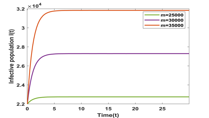
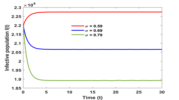
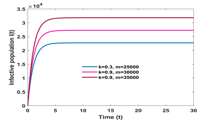
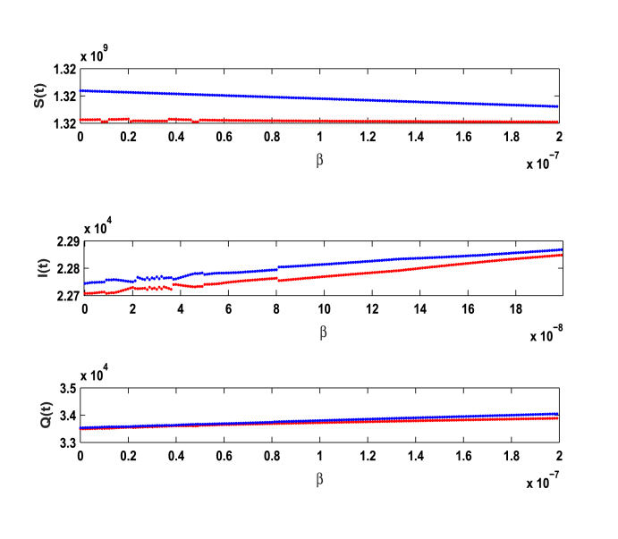
We have calculated the equilibrium points of the system without immigration when complete lockdown was imposed by the government. In this case system possess two equilibrium points, one is disease free equilibrium point (1.282750 × 10⁹, 0, 0) and the other is the pandemic equilibrium point (1.28237 × 10⁹, 14.03000, 35.59000). Basic reproduction ratio R₀ is computed and is found to be 3.80. All the conditions of local and global asymptotic stability are verified by the above set of parameters. However, when lockdown is not imposed and immigration of individuals is allowed in the system then our model possess only one equilibrium point given by (1.32976 × 10⁹, 22745.39525, 33564.48733). Above set of parameters satisfy the conditions of local stability of the equilibrium point and persistence. In addition, to study the impact of various parameters on the infective population we plotted time series graphs of infective population. Figure 2 shows the variation of infective population with time for different number of immigrants. It is observed that infective population rise significantly with the increase in number of immigrants. Hence it is imperative to impose complete/partial lockdown in the country to decrease the number of infective population. In the absence of lockdown, the spread of COVID-19 cases will shoot up. From Fig. 3, we determine the impact of transition rate of infective individuals to quarantine compartment. It is observed that as transition rate increases number of infective individuals decrease. It implies that the rate σ at which infective individuals are quarantined plays a significant role in controlling the number of infective population and hence to control the disease. Fig. 4, manifests the impact of contact tracing on the population of infective individuals. It is observed from the figure that although number of infective individuals increase with the number of immigrants in the system yet their population can be kept under control by contact tracing. Hence, contact tracing and quarantine play an important role in keeping the disease under control when government unlocks or in case of partial lockdown conditions. Fig. 5 shows variation of susceptible, infective and quarantined population with time for different values of transmission rate of infection. From the figure we infer that as transmission rate of infection increases infective, population rises and hence quarantined population also rises, leading to decrease in susceptible population. In addition, we observe that it is a bifurcation parameter.

Fig. 2.

Variation in infective population with no. of migrants ‘m’.

Fig. 3.

Effect of transition rate ′σ′ on infective population.

Fig. 4.

Effect of contact tracing ‘k′ on infective population.

Fig. 5.

Effect of transmission rate β on susceptible, infective and quarantined population.

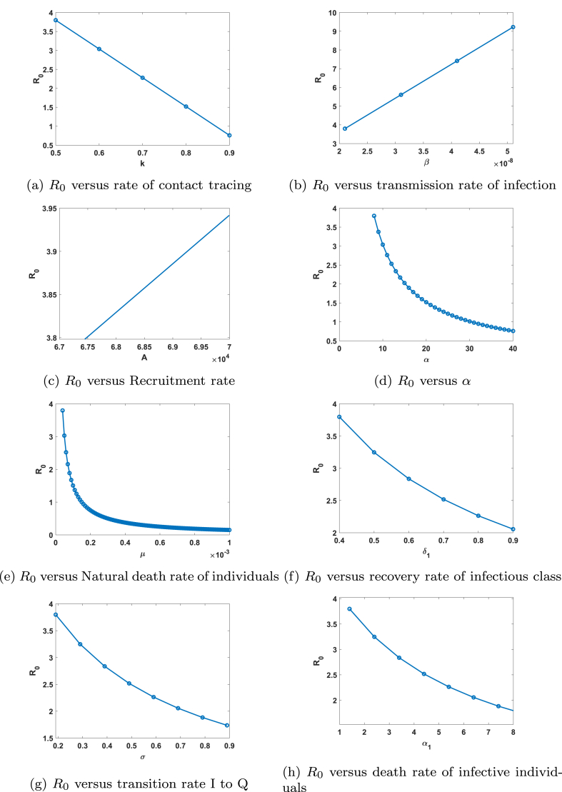
To determine the impact of various parameters on the threshold parameter Basic Reproduction number, we plot figures depicting variation of R₀ with different parameters. In Fig. 6a, b, c and d we plot the variation of R₀ with rate of contact tracing k, transmission rate of infection β, recruitment rate A, half saturation constant α respectively.

Fig. 6.

Effect of different parameters on Reproduction number ‘R₀′.

We observe that with the increase in rate of contact tracing k to 0.9, basic reproduction number reduces below one. Hence by the practice of contact tracing disease can be controlled. Further with the increase in β, basic reproduction number continues to rise linearly. This implies that if transmission rate of infection will rise continuously, we will not be able to control the disease and it will spread in the population. Further R₀ rises with the increase in recruitment rate A. Reproduction ratio R₀ decreases with the increase in half saturation constant, α. In e, f, g and h display the variation of reproduction number with natural mortality rate μ, recovery rate of infective’s δ₁, transition rate of infective’s to quarantined class σ and disease related death rate of infective individuals α₁. It is observed that R₀ decreases with the increase in these parameter values. Thus, from this study we confer that basic reproduction ratio can be reduced and maintained below one by controlling the parameters k, α, μ, β, σ, δ₁ and α₁.

7. Result and discussion

This paper represents a nonlinear mathematical model to study the impact of lockdown on the spread of COVID-19 with significant preventive measures adopted by the Indian government to control the spread of disease. Study of the proposed model is divided into two phases; complete lockdown state and partial lockdown or unlocked state. Qualitative analysis of the model in both the cases is performed and basic reproduction ratio is determined through next generation matrix approach. Nature of equilibrium points is found to be dependent significantly on the basic reproduction number. It is observed that disease free equilibrium is both locally and globally stable if basic reproduction number is less than one and pandemic equilibrium exists only if basic reproduction number is greater than one. However, in the case of unlocked or partial lockdown state, diseases free equilibrium does not exist and disease will persist in the system. Thus, lockdown is most important measure to be imposed strictly until infection dies out from the country to reduce the infection to zero. Local stability of the pandemic equilibrium and conditions of persistence are determined in case of unlock or partial lockdown state. Further, to justify the analytical findings, numerical simulation is performed and graphs are plotted. It is observed that infective population rise significantly with the increase in number of immigrants in case of partial lockdown state. However, this situation can be kept under control by contact tracing and quarantine, since numerical simulation confirms the decrease in infective population with the increase in their rate. Hence, contact tracing and quarantine play an important role is keeping the disease under control in case of unlock or partial lockdown state. But in order to completely eradicate the disease, lockdown is most important measure to be followed by the government. In addition, we have identified the significant parameters by which basic reproduction number can be reduced and maintained below one. Contact tracing and half saturation constant play an important role in keeping the basic reproduction number below one along with the transmission rate of infection, susceptible population in disease free state and infectious period of an infective individual. Sensitivity analysis of the basic reproduction number is carried out and sensitivity index of each parameter is determined. It is observed from the analysis that transmission rate of infection is most sensitive factor in basic reproduction number and acts as transcritical bifurcation parameter. Our study reveals that complete lockdown is mandatory for reducing the infection to zero and control in immigration of population in the system is an outstanding step to control the spread of the disease. Still, the complete lockdown is not the ultimate solution since it may cause financial crisis in the near future and hence it is not possible to implement complete lockdown in highly dense country like India for a long tenure. Therefore, keeping an eye on the immigration of infective population in the country, government must emphasize on other preventive measures too like increase in rate of contact tracing and quarantining the confirmed cases of COVID-19 on a regular basis until infection dies out.

Declaration of competing interest

The authors declare that they have no known competing financial interests or personal relationships that could have appeared to influence the work reported in this paper.

Handling editor: Dr. J Wu

References

- Aparicio J.P., Hernandez J.C. Preventive treatment of tuberculosis through contact tracing. Contemporary Mathematics. 2006;410:17–20. [Google Scholar]
- Arriola L.M., Hyman J.M. Technical report; 2003. Forward and adjoint sensitivity analysis: With applications in dynamical systems. [Google Scholar]
- Barnett E.D., Walker P.F. Role of immigrants and migrants in emerging infectious diseases. Medical Clinics of North America. 2008;92(6):1447–1458. doi: 10.1016/j.mcna.2008.07.001. [DOI] [PMC free article] [PubMed] [Google Scholar]
- Bhola J., Venkateswaran V.R., Koul M. medrxiv; 2020. Corona epidemic in Indian context: Predictive mathematical modelling. 200471753. [Google Scholar]
- Binti H.F.A., Lau C., Nazri H., Ligot D.V., Lee G., Tan C.L. CoronaTracker: World-wide COVID-19 outbreak data analysis and prediction, [preprint] Bull World Health Organ, E-pub. 2020;19:255695. [Google Scholar]
- Brauer F., Castillo C.C. Springer; Berlin: 2001. Mathematical models in population biology and epidemiology. [Google Scholar]
- Carr J. Springer Verlag; Newyork: 1981. Application of center manifold Theory. [Google Scholar]
- Chavez C.C., Feng Z., Huang W. On the computation of ro and its role on. Mathematical approaches for emerging and reemerging infectious diseases: An introduction. 2002;1:229. [Google Scholar]
- Chen S.C., Chang C.F., Liao C.M. Predictive models of control strategies involved in containing indoor airborne infections. Indoor Air. 2006;16(6):469–481. doi: 10.1111/j.1600-0668.2006.00443.x. [DOI] [PubMed] [Google Scholar]
- Cowling B.J., Park M., Fang V.J., Wu P., Leung G.M., Wu J.T. Preliminary epidemiologic assessment of mers-cov outbreak in South Korea May–June 2015. Euro Surveillance. 2015;20(25):21163. doi: 10.2807/1560-7917.es2015.20.25.21163. [DOI] [PMC free article] [PubMed] [Google Scholar]
- Day T., Park A., Madras N., Gumel A., Wu J. When is quarantine a useful control strategy for emerging infectious diseases. American Journal of Epidemiology. 2006;163(5):479–485. doi: 10.1093/aje/kwj056. [DOI] [PMC free article] [PubMed] [Google Scholar]
- Driessche P.V.D., Watmough J. Reproduction numbers and sub-threshold endemic equilibria for compartmental models of disease transmission. Mathematical Biosciences. 2002;180:2948. doi: 10.1016/s0025-5564(02)00108-6. [DOI] [PubMed] [Google Scholar]
- Eunha S. A note on epidemic models with infective immigrants and vaccination. Mathematical Biosciences and Engineering. 2006;3(3):557. doi: 10.3934/mbe.2006.3.557. [DOI] [PubMed] [Google Scholar]
- Fraser C., Riley S., Anderson R.M., Ferguson N.M. Factors that make an infectious disease outbreak controllable. Proceedings of the National Academy of Sciences. 2004;101(16):6146–6151. doi: 10.1073/pnas.0307506101. [DOI] [PMC free article] [PubMed] [Google Scholar]
- Jia L. 2020. Prediction and analysis of coronavirus disease. arXiv preprint arXiv:2003.05447. [Google Scholar]
- Koonprasert S., Chananngam N. Global stability and sensitivity analysis of SEIQR worm virus propagation model with quarantined state in mobile internet. Global Journal of Pure and Applied Mathematics. 2017;13(7):3833–3850. [Google Scholar]
- Kwok K.O., Arthur T., Vivian W.I., Wei W.H., Park E., Kiong Y., Steven R. Epidemic models of contact tracing: Systematic review of transmission studies of severe acute respiratory syndrome and Middle East respiratory syndrome. Computational and Structural Biotechnology Journal. 2019;17:186–194. doi: 10.1016/j.csbj.2019.01.003. [DOI] [PMC free article] [PubMed] [Google Scholar]
- Liang K. Mathematical model of infection kinetics and its analysis for COVID-19, SARS and MERS. Infection, Genetics and Evolution. 2020;82:104306. doi: 10.1016/j.meegid.2020.104306. [DOI] [PMC free article] [PubMed] [Google Scholar]
- Li Q., Guan X., Peng W., Zhou X., Tong Y. Early transmission dynamics in Wuhan, China, of novel coronavirus-infected pneumonia. New England Journal of Medicine. 2020;1–9 doi: 10.1056/NEJMoa2001316. [DOI] [PMC free article] [PubMed] [Google Scholar]
- Mandal M., Jana S., Nandi S.K., Khatua A., Adak S., Kar T.K. Solitons and Fractals; 2020. A model based study on the dynamics of COVID-19: Prediction and control, Chaos; p. 109889. [DOI] [PMC free article] [PubMed] [Google Scholar]
- Marimuthu Y., Nagappa B., Sharma N., Basu S., Chopra K.K. COVID-19 and tuberculosis: A mathematical model based forecasting in Delhi, India. Indian Journal of Tuberculosis. 2020;67(2) doi: 10.1016/j.ijtb.2020.05.006. [DOI] [PMC free article] [PubMed] [Google Scholar]
- Mohsen M., Wraith M.R. Travel Medicine and Infectious Disease; 2020. Time series modelling to forecast the confirmed and recovered cases of COVID-19; p. 101742. [DOI] [PubMed] [Google Scholar]
- Ndairou F., Area I., Nieto J.J., Torres D.F.M. Mathematical modeling of COVID-19 transmission dynamics with a case study of Wuhan. Chaos, Solitons & Fractals. 2020;135 doi: 10.1016/j.chaos.2020.109846. 109846. [DOI] [PMC free article] [PubMed] [Google Scholar]
- Nyabadza F., Hove-Musekwa S.D. From heroin epidemics to methamphetamine epiepidemics: Modelling substance abuse in a South African province. Mathematical Biosciences. 2010;225:132140. doi: 10.1016/j.mbs.2010.03.002. [DOI] [PubMed] [Google Scholar]
- Pal D., Ghosh D., Santra P.K., Mahapatra G.S. medRxiv; 2020. Mathematical analysis of a COVID-19 epidemic model by using data driven epidemiological parameters of dseases spread in India. [DOI] [PMC free article] [PubMed] [Google Scholar]
- Spiteri G., Fielding J., Diercke M. First cases of coronavirus disease 2019 (COVID-19) in the WHO European region, 24 January to 21 February 2020. Euro Surveillance. 2020;25(9):2000178. doi: 10.2807/1560-7917.ES.2020.25.9.2000178. [DOI] [PMC free article] [PubMed] [Google Scholar]
- Vega D.I. Lockdown, one, two, none, or smart. Modeling containing covid-19 infection: A conceptual model. The Science of the Total Environment. 2020;730 doi: 10.1016/j.scitotenv.2020.138917. 138917. [DOI] [PMC free article] [PubMed] [Google Scholar]
- Wang W. Population dispersal and disease spread. Discrete and Continuous Dynamical Systems - Series B. 2004;4(3):797–804. [Google Scholar]
- Wang W., Zhao X.Q. An epidemic model with population dispersal and infection period. SIAM Journal on Applied Mathematics. 2006;66(4):1454–1472. [Google Scholar]
- Yang J.Y., Zhang F.Q., Wang X.Y. SIV epidemic models with age of infection. International Journal of Biomathematics. 2009;2(1):61–67. [Google Scholar]