Disentangling time series between brain tissues improves fMRI data quality using a time-dependent deep neural network

Abstract

Functional MRI (fMRI) is a prominent imaging technique to probe brain function, however, a substantial proportion of noise from multiple sources influences the reliability and reproducibility of fMRI data analysis and limits its clinical applications. Extensive effort has been devoted to improving fMRI data quality, but in the last two decades, there is no consensus reached which technique is more effective. In this study, we developed a novel deep neural network for denoising fMRI data, named denoising neural network (DeNN). This deep neural network is 1) applicable without requiring externally recorded data to model noise; 2) spatially and temporally adaptive to the variability of noise in different brain regions at different time points; 3) automated to output denoised data without manual interference; 4) trained and applied on each subject separately and 5) insensitive to the repetition time (TR) of fMRI data. When we compared DeNN with a number of nuisance regression methods for denoising fMRI data from Alzheimer’s Disease Neuroimaging Initiative (ADNI) database, only DeNN had connectivity for functionally uncorrelated regions close to zero and successfully identified unbiased correlations between the posterior cingulate cortex seed and multiple brain regions within the default mode network or task positive network. The whole brain functional connectivity maps computed with DeNN-denoised data are approximately three times as homogeneous as the functional connectivity maps computed with raw data. Furthermore, the improved homogeneity strengthens rather than weakens the statistical power of fMRI in detecting intrinsic functional differences between cognitively normal subjects and subjects with Alzheimer’s disease.

1. Introduction

Functional magnetic resonance imaging (fMRI) based on the blood-oxygen-level-dependent (BOLD) signal is a prominent technique for investigating human brain function. The BOLD signal is an indirect measure of neuronal activity which occurs when the subject is scanned during task-based and task-free (resting-state) conditions. However, the reliability and reproducibility of fMRI is compromised by a large proportion of noise from multiple sources, including head-motion related artifacts, cardiac and respiratory oscillations, thermal noise inherent to electrical circuits, changes in blood pressure, and other factors (Bianciardi et al., 2009; Caballero-Gaudes and Reynolds, 2017; Murphy et al., 2013). Multiple studies have demonstrated that these noise sources can adversely affect the results and interpretations of task-based or resting-state fMRI experiments (Birn et al., 2006; Chang et al., 2009; Van Dijk et al., 2012). An advanced method to substantially improve fMRI data quality will advance brain function research by allowing more accurate mapping of human brain function.

Extracting nuisance regressors from fMRI data or modeling the noise from externally recorded data (physiological data in most cases) and then regressing out these confounding signals is a commonly used technique for improving fMRI data quality. Many regression-based methods have been developed to correct the confounding signal induced by head motion or major physiological noise oscillations, such as cardiac and respiratory fluctuations. The six rigid-body affine transformation parameters (R=[X Y Z pitch yaw roll]) estimated from aligning fMRI volumes have been commonly used to address head-motion related artifacts (Friston et al., 1996; Johnstone et al., 2006). The first-order temporal derivatives (R’) and squares (R²) of these six realignment parameters were also used in nuisance regression to remove spin history related aspects of head motion (Friston et al., 1996; Satterthwaite et al., 2013). However, the change of image intensity generated by head motion might not be properly explained by the realignment parameters. These regressors have over-simplified the influence of head motion in fMRI data (Caballero-Gaudes and Reynolds, 2017). Physiological noise in fMRI data is usually addressed by constructing nuisance regressors with externally recorded physiological data (Birn et al., 2008; Chang et al., 2009; Glover et al., 2000; Harvey et al., 2008; Shmueli et al., 2007; Tijssen et al., 2014). Instead of explicitly modeling a particular noise source, data-driven methods were developed without assuming any parametric noise model. Using the mean whole-brain time series (namely global signal) (Anderson et al., 2011; Jo et al., 2010) and the principal component decompositions from white matter (WM) and cerebrospinal fluid (CSF) time series (namely anatomic Compcor (aCompcor) from Behzadi et al. (2007)) as nuisance regressors are two typical examples, which assume that the signal of interest in fMRI data mostly comes from gray matter (GM) tissue and that GM shares similar noise characteristics with WM and CSF. The inclusion of global signal as a regressor has been heavily debated in recent years (Murphy et al., 2009; Power et al., 2018; Saad et al., 2012; Weissenbacher et al., 2009) because it could artificially introduce anticorrelation between brain regions. Methods based on principal component analysis (Kay et al., 2013) and independent component analysis (Griffanti et al., 2014; Pruim et al., 2015; Salimi-Khorshidi et al., 2014) were recently developed for reducing noise in fMRI data by regressing out certain components, which were manually or automatically labelled as noise. Regardless of how regressors are obtained, increasing the number of regressors may reduce more noise variance from fMRI data but could lead to a higher risk of substantially removed BOLD signal as well. In addition, nuisance regression could contaminate fMRI data because the regression coefficient is heavily driven by one particular frequency band (Chen et al., 2017).

Artificial intelligence technique has recently gained a lot of interest in neuroscience research (Marblestone et al., 2016; Yang et al., 2020a). In this study, we have used this technique to develop a non-regression-based denoising neural network (DeNN) for automatically alleviating the influence of noise in fMRI data. Similar to the assumption in aCompcor that GM and non-GM time series share similar noise but no functional signal of interest is expected in non-GM regions, DeNN is designed with the hypothesis that disentangling time series between GM and non-GM voxels can substantially reduce noise in fMRI data. We compared DeNN with multiple nuisance regression methods (Behzadi et al., 2007; Friston et al., 1996; Murphy et al., 2009; Yang et al., 2019) by analyzing standard resting-state fMRI data from the Alzheimer’s Disease Neuroimaging Initiative (ADNI, http://adni.loni.usc.edu/). Then, we examined positive and negative correlations in resting-state networks, evaluated the similarity of functional connectivity maps between subjects, and compared the group difference of graph theory measures between cognitively normal (CN) subjects and subjects with Alzheimer’s disease (AD). Limited analysis was also carried out with multi-band fMRI data from Human Connectome Project (HCP) (Van Essen et al., 2013).

2. Materials and methods

Subject Demographics and Image Acquisition.

Data acquired at the baseline visits were included from 193 participants in the multi-site ADNI project (http://adni.loni.usc.edu/), with the inclusion criterion that participants were diagnosed as having normal cognition, early mild cognitive impairment (eMCI), or AD, with resting-state fMRI data and structural MRI data available. The study was approved by each participating ADNI site’s local Institutional Review Boards, as documented on the ADNI website. All participants gave written, informed consent. The subject ID, imaging data ID, and other demographical information are listed in Table S1. The summary of the demographic information, including diagnosis, age, gender, handedness, education, and MMSE scores are listed in Table 1. All subjects were scanned on 3.0-Tesla Philips MRI scanners. The magnetization prepared rapid acquisition gradient echo (MP-RAGE) sequence was used to acquire T1-weighted structural images. The structural MRI scans were collected with a 24cm field of view and a resolution of 256 × 256 × 170 to yield a 1 × 1 × 1.2mm³ voxel size. The resting-state fMRI data were acquired from a regular echo-planar imaging sequence with 140 time points, TR/TE=3000/30 ms, flip angle=80 degrees, 48 slices, spatial resolution=3.3 × 3.3 × 3.3mm³ and imaging matrix=64 × 64. More details about the MRI protocol can be found on the ADNI website.

Table 1.

Demographic information of the 193 subjects from the ADNI cohort.

	CN	eMCI	AD
Age (years ± std)	75.9±5.6	73.6±7.0	73.5±8.4
Handedness (Right/Left)	55/5	63/7	59/4
Education (years ± std)	16.5±2.4	15.9±2.8	15.9±2.7
Gender (Male/Female)	27/33	39/31	36/27
MMSE ± std	27.8±5.4	27.0±5.4	22.1±2.9

General fMRI preprocessing.

Functional and structural MRI imaging data were processed with SPM12 (https://www.fil.ion.ucl.ac.uk/spm/) and ANTs (version 2.1.0, http://stnava.github.io/ANTs/) toolboxes. The first five volumes of fMRI data were discarded to avoid data with unsaturated T1 signals. The following fMRI preprocessing steps were applied: (i) slice-timing correction (SPM12); (ii) rigid-body realignment of all fMRI volumes to mean fMRI image using 7th order B-Spline interpolation (SPM12); (iii) co-registration of mean fMRI image to the skull-stripped T1 structural image (command ANTS 3 -m MI[T1_dir, meanfmri_dir,1,32] in ANTs); (iv) standard space normalization of T1 image to the MNI152 2mm template (command antsRegistrationSyN.sh -d 3 -f MNI152_dir -m T1_dir in ANTs); (v) transforming all fMRI volumes to MNI space with the transformation information from (iii) and (iv) (command antsApplyTransforms in ANTs). Nuisance regression or DeNN denoising was applied after the general fMRI preprocessing step.

DeNN network architecture.

We observed that the time series denoised by our previous deep learning strategy (Yang et al., 2019) still contained some band structure visible in the gray plot of time series, introduced by head motion and other noise sources (Figure S1). The reason is possibly twofold. First, this denoising strategy was regression-based, which could be insufficient for modeling spatial variation of motion artifacts across the brain. Second, the same network parameters were used for all time points in our previous neural network without considering the uniqueness of noise at each time point. The property of temporal independence could have reduced the effectiveness of our previously developed deep neural network in addressing abrupt motion and other irregular noise variances. A non-regression-based deep neural network with a time-dependent layer could potentially further improve fMRI data quality. Therefore, a deep neural network with this property, namely DeNN, is introduced in this study.

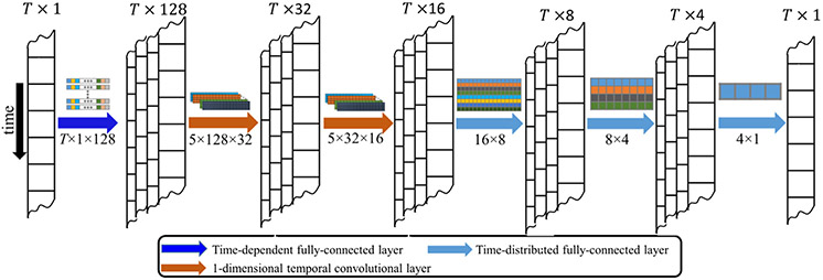
DeNN consists of six layers in a sequential order, namely a novel time-dependent fully-connected layer proposed in this study, two 1-dimensional temporal convolutional layers, and three time-distributed fully-connected layers, as shown in Fig. 1. DeNN is fed with original time series after general preprocessing steps and outputs denoised data directly, instead of outputting nuisance regressors as in Yang et al. (2019).

Fig. 1.

Architecture of the denoising neural network (DeNN). DeNN consists of one novel time-dependent fully-connected layer (dark blue arrow), two 1-dimensional temporal convolutional layers (brown arrow), and three time-distributed fully-connected layers (light blue arrow) in a sequential order. The input to the network is the voxel time series, and the output is the denoised time series. The parameters (constant term is omitted) for each layer are illustrated above the arrow, with each color representing the parameters for an output channel. The dimension of the parameters for each layer is marked under the arrow.

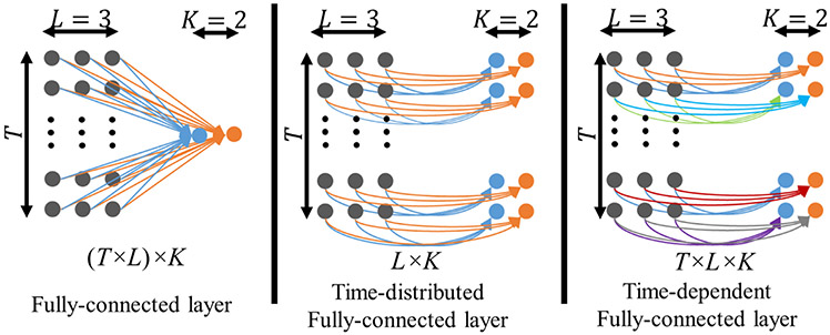
The schematic diagrams of different fully-connected layers with T × L input nodes and K output nodes is shown in Fig. 2, where T, L, and K represent the number of time points, the input channels, and the output channels, respectively. The standard fully-connected layer connects all input nodes, with the output nodes ignoring the temporal property of the data (left panel of Fig. 2). A time-distributed fully-connected layer applies a fully-connected operation with the same parameters to each time point separately (middle panel of Fig. 2). In contrast, the time-dependent fully-connected layer has a fully-connected operation to each time point with different parameters (right panel of Fig. 2). The number of parameters in the time-dependent layer linearly increases with the number of time points acquired in fMRI data, resulting in a higher computational cost for longer time series. The temporal convolutional layers can be treated as a set of temporal filters with unknown pass bands, which are learned from the data without manually specifying a fixed frequency threshold. We have demonstrated this property in previous task fMRI denoising work (Yang et al., 2020b). Learning filtering properties from data is particularly important because the commonly used frequency threshold of 0.1 Hz in fMRI preprocessing remains a topic of debate (Boubela et al., 2013; Chen and Glover, 2015; Cordes et al., 2001).

Fig. 2.

Schematic diagrams of a fully-connected layer (left), a time-distributed fully-connected layer (middle) and a time-dependent fully-connected layer. The fully-connected layer links all (T × L) input nodes to each output node leading to (T × L) × K parameters in the layer and K output nodes. The time-distributed fully-connected layer links the L input nodes with K output nodes at each time point with the same parameter leading to L × K parameters and the T × K output dimension. The time-dependent fully-connected layer links the L input nodes with K output nodes at each time point with distinct parameters, leading to T × L × K parameters and T × K output dimension.

The temporal convolutional layers used in this study (layers 2 and 3) have 1-dimensional filters with a filter size of five time points. Zero padding is used to ensure the output time series have the same number of time points as the input time series. These convolutional layers output each time point with data from neighboring time points and the same filters are applied for all time points. They are effective for reducing periodic or pseudoperiodic noise and have been successfully implemented in our previous work (Yang et al., 2020b). However, temporal convolutional layers have a risk of propagating temporally limited noise variance (e.g. abrupt motion) through the entire time series and complicating the denoising process. Therefore, a time-dependent fully-connected layer is applied before the temporal convolutional layer to address irregular noise. For the ADNI data, the time-dependent fully-connected layer was specified with 128 units, and the first and second temporal convolutional layers were specified with 32 and 16 filters, respectively. Following the temporal convolutional layers, three time-distributed fully-connected layers were specified with 8, 4, and 1 filters, respectively, in sequential order. These time-distributed fully-connected layers determine the weight of the multiple channels from the second temporal convolutional layer and output the denoised time series. Note that a time-distributed fully-connected layer is equivalent to a temporal convolutional layer with a filter size of one. The last layer has a single filter to ensure one output time series for each voxel. The dimension of input data, output of each layer, and the network parameters in each layer are marked in Fig. 1 (the dimension for the number of samples is omitted).

Customized cost function for DeNN.

The cost function provides a criterion to optimize the parameters in the network during the iteration step. Many cost functions have been developed for classification or regression in machine learning and deep learning applications, such as mean squared error, mean absolute percentage error, cross entropy, Poisson, and cosine proximity. Implementation of these cost functions requires known true values or classes. However, the true BOLD signal in fMRI data is unknown, and extracting the underlying BOLD signal is difficult, if not impossible, especially for resting-state data. Therefore, a customized cost function that does not require the knowledge of the underlying BOLD signal is preferred.

The rationality embedded in aCompcor (Behzadi et al., 2007) is that GM tissue shares similar noise properties with non-GM tissue (including WM and CSF), and removing the common variance can improve data quality. With similar rationality, the cost function for DeNN is designed to minimize the correlation between GM and non-GM time series. DeNN is trained by first arbitrarily pairing one GM voxel with one non-GM voxel. Each paired time series is treated as a sample and assigned to different batches. In each batch, let Y_raw denotes the original fMRI data within the gray matter mask (GM mask) and ${\tilde{\mathit{Y}}}_{raw}$ denotes the paired time series within eroded white matter or ventricle mask (nonGM mask). Erosion is applied to reduce the risk of BOLD signal included in ${\tilde{\mathit{Y}}}_{raw}$ because of partial volume effect. During the learning process, Y_raw and ${\tilde{\mathit{Y}}}_{raw}$ share the same network (including network architecture and parameters) and are fed to the network alternatingly in each iteration. Each iteration will then provide the corresponding output data Y_denoise and ${\tilde{\mathit{Y}}}_{denoise}$. The cost function $\mathcal{L}=\mathcal{L}({\mathit{Y}}_{denoise},{\tilde{\mathit{Y}}}_{denoise})$ is defined as the sum of the correlation magnitude between paired time series given by

$$\mathcal{L}({\mathit{Y}}_{denoise},{\tilde{\mathit{Y}}}_{denoise})=\sum _{\mathit{y}\in {\mathit{Y}}_{denoise},\tilde{\mathit{y}}\in {\tilde{\mathit{Y}}}_{denoise}}\mid \text{corr}(\mathit{y},\tilde{\mathit{y}})\mid ,$$ (1)

where [y, $\tilde{\mathit{y}}$] is one paired time series from [Y_denoise, ${\tilde{\mathit{Y}}}_{denoise}$].

DeNN is optimized for each subject separately, because the characteristics of noise is highly subject-dependent, including the severity of head motion, rate and stability of cardiac and respiratory pulses, and other unknown subject-specific factors. Since there are hundreds of thousands of voxels in a standard fMRI acquisition protocol, the large number of voxels makes it feasible to train a subject-specific DeNN model.

DeNN training and calibration.

Since GM and nonGM voxels are paired to calculate the customized loss function, the same number of voxels within GM and nonGM masks are required to be the input samples to the network. The voxels within GM are randomly paired with voxels within nonGM and the extra voxels within GM or nonGM mask are discarded in the following optimization. There are about 50,000 paired time series for each subject, which are the input to the network. 90% of the paired-voxels are assigned randomly to the training set to update parameters, and the remaining 10% of the paired-voxels are assigned to the validation set to monitor whether or not the network suffers from over-fitting or under-fitting, leading to either high bias or variance, respectively. There is no independent testing set, because the noise variance in each fMRI session is unique, and DeNN is trained to specifically address the noise existing in the training set. Therefore, once the model is trained, the whole brain original fMRI data (including the time series used or not used in training and validation set) are the input to the model, with the output of denoised time series.

The initial parameters are randomly sampled from the Xavier uniform initializer (Glorot and Bengio, 2010). The parameters are updated with the Adam stochastic gradient-based optimization algorithm (Kingma and Ba, 2014), which adapts the parameter learning rates by taking advantage of both the average first moment (mean) and the average of the second moments of the gradients (uncentered variance). The Adam optimizer is parameterized with learning rate η=0.01, learning rate decay γ=0.05, exponential decay rate for the first moment estimates β₁ = 0.9 and exponential decay rate for the second moments estimates β₂ = 0.999. The parameters and their learning gradients are updated with each batch of 500 paired time series (or samples). Thus, the input data Y_raw and ${\tilde{\mathit{Y}}}_{raw}$ in each batch have the same dimension of 500 × T × 1, where the singleton dimension “1” represents the number of channels. One epoch is defined as running through all batches once and the network is set to run up to 50 epochs, with the early stopping criterion that the network stops training if the cost for the validation data does not reduce in the last five epochs. The number of layers in the network is heuristically selected. To determine the network architecture for ADNI data, we have applied DeNN on ten randomly selected subjects multiple times with gradually increasing layer sizes until the mean cost does not show considerable decrease with larger layer sizes, which allows the network to be relatively time-efficient and effective. The same network architecture is used for all subjects to avoid extensive human effort.

Nuisance regressors.

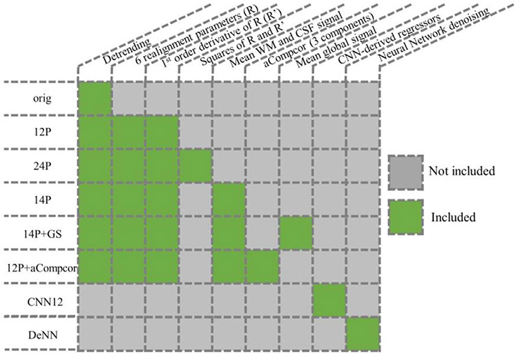
The nuisance regressors used in this study include the linear detrending regressor, six rigid-body realignment parameters R, first order derivative of R (R’), squares of R and R’, mean WM and CSF time series, aCompcor, and the global signal (GS). Different combinations of these regressors lead to the five datasets named as 12P, 24P, 14P, 14P+GS, and 12P+aCompcor. As shown in Fig. 3, 12P consists of 12 regressors, including the six realignment parameters R and their first order derivative R’. 24P consists of the 12P and its squared regressors. 14P indicates 14 regressors consisting of regressors in 12P, and mean WM and CSF time series. aCompcor is applied with the top three principal components from WM and CSF as nuisance regressors (in total 6 regressors). Erosion is carried out to generate WM and CSF masks to avoid the partial volume effect. Nuisance regression is applied after general preprocessing steps.

Fig. 3.

Different denoising strategies for fMRI data.

Graph theoretical network analysis.

The mean region of interest (ROI) time series is computed with 94 cortical and subcortical ROIs from the revised AAL atlas (AAL2) (Tzourio-Mazoyer et al., 2002), and then the functional connectivity map is constructed with Pearson’s correlation. To evaluate how different denoising strategies influence the power of detecting brain function difference between AD and CN, graph theoretical analysis is performed, and 2-sample t-test is applied to evaluate the group difference with age, gender, handedness and education as covariates. The graph theoretical network analysis is carried out using the GRETNA toolbox (version 2.0.0) (Wang et al., 2015). 11 network metrics are obtained for analysis, including assortativity, betweenness centrality, degree centrality, global efficiency, local efficiency, clustering efficiency C_p, γ, λ, path length L_p, σ, and synchronization. The nodal network metrics are averaged across all ROIs to generate a single measure for comparison.

3. Results

We analyzed data from 193 ADNI subjects to explore the extent to which the denoising steps influence fMRI data quality. In this section, we demonstrate the performance of different strategies qualitatively by comparing the gray plot of the time series and quantitatively by conducting the functional connectivity (FC) analysis. A group comparison of network metrics between CN and AD presents intermediate evidence to further support our hypothesis.

Visualization of denoised time series.

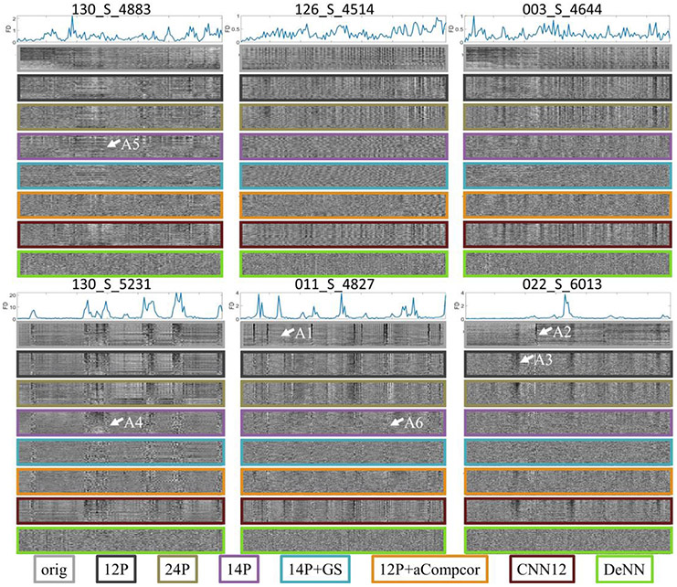
Time series from six example subjects after different denoising strategies are shown in Fig. 4. These subjects are selected to demonstrate different noise characteristics and the varying performance of different denoising strategies. The gray plots of all subjects can be seen in the Supplementary. The framewise displacement (FD) (Power et al., 2012) derived from rigid head motion estimation, along the time point (x-axis), is shown in the top panel. The higher FD value means that the rigid head motion is more severe. The original whole-brain time series and the time series processed by 12P, 24P, 14P, 14P+GS, 12P+aCompcor and DeNN are presented in a descending order. Motion artifact, signal drift, and noise fluctuation introduced by unknown sources are observed in these subjects. Head motion corrupts fMRI data with varying duration (note width of dark band in Fig. 4). A large motion might not have a visually obvious effect in fMRI data (e.g. arrow A1), but a small motion could considerably change the signal (e.g. arrow A2). By only regressing out rigid-body realignment parameters and their variants (e.g. 12P and 24P), motion artifacts were insufficiently addressed. These regressors can even be detrimental for some time points (e.g. arrow A3). The band structure in the gray plot indicates similar noise fluctuation widespread across the entire brain. This particular noise structure was alleviated by including additional regressors extracted from fMRI data, such as global signal, mean WM, and CSF time series or principal components from WM and CSF time series (aCompcor). However, such noise artifacts remained noticeable (e.g. arrow A4–6). In contrast, DeNN visually showed substantially reduced band-structure artifacts and achieved more homogeneous time series. Besides band structure variation, the pseudoperiodic variations in subjects 126_S_4514 and 003_S_4644 were also considerably reduced. The gray plots for all ADNI subjects were included in the Supplementary. In addition to the time series achieved by the methods in Fig. 4, the denoised time series by running DeNN without the time-dependent fully-connected layer (all the other layers remain the same, named DeNN0) were also plotted in the Supplementary, which clearly demonstrated the necessity of the time-dependent fully-connected layer in DeNN to reduce band structure variance in fMRI data.

Fig. 4.

Gray plot of the time series from six example subjects. The top panel for each subject shows the framewise displacement (in mm) derived from rigid head motion estimation. The remaining panels show the time series with voxels along the y-axis and time points along the x-axis.

Seed-based functional connectivity analysis.

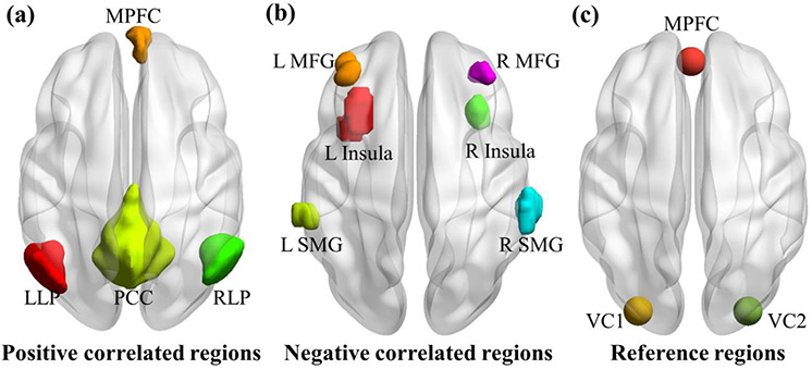
A quantitative comparison of different denoising strategies was applied by conducting a functional connectivity analysis. We predefined a PCC seed as a 10-mm sphere around the coordinate (−7, −55, 27) in Montreal Neurological Institute (MNI) space to select regions having positive and negative correlations with the PCC seed. The whole-brain functional connectivity map between voxel-wise time series and the PCC seed was calculated for each subject. Four ROIs were identified as positively correlated with the PCC seed, and six ROIs were identified as negatively correlated with the seed by following Fox et al. (2005). The positive-correlated ROIs include PCC, the medial prefrontal cortex (MPFC), left lateral parietal cortex (LLP), and right lateral parietal cortex (RLP), which are within the default mode network. The six anticorrelated ROIs include the bilateral insula, the bilateral middle frontal gyrus (MFG), and the bilateral supramarginal gyrus (SMG), which are within the task positive network (TPN) and consistent with the task-positive regions observed in Fox et al. (2005). The correlation coefficients between ROIs and the PCC seed were converted to a normal distribution by Fisher’s r-to-z transformation. The four regions showing significant positive correlation and the six regions showing significant negative correlation with the PCC seed are shown in Fig. 5a and Fig. 5b, respectively.

Fig. 5.

(a) Four positive-correlated ROIs; (b) six negative-correlated ROIs; (c) two reference regions in visual cortex (VC1 and VC2), which are not expected to have connectivity with the MPFC seed.

The specificity defined as

$$S_{target}=\frac{\mid Z_{target}\mid -\mid Z_{reference}\mid }{\mid Z_{target}\mid +\mid Z_{reference}\mid }\in [-1,1],$$ (2)

by following Chai et al. (2012) is used to compare the seed-based connectivity values achieved by different denoising strategies, where Z is the Fisher r-to-z transformed connectivity value. In this equation Z_target refers to the connectivity from the MPFC to the positive-correlated or anticorrelated ROIs and Z_reference refers to the mean connectivity from MPFC to the two reference regions in visual cortex. MPFC is expected to be functionally uncorrelated with the visual area (Biswal et al., 1995; Chai et al., 2012; Fox et al., 2005; Van Dijk et al., 2010). The connectivity between MPFC seed (10-mm sphere centered at coordinates (−1, 49, −2) in MNI space) and two visual regions (10-mm spheres centered at coordinates (−30, −88, 0) and (30, −88, 0)) (see Fig. 5c) is evaluated, and the mean connectivity between these two visual regions and MPFC seed is used as the reference connectivity to compute specificity.

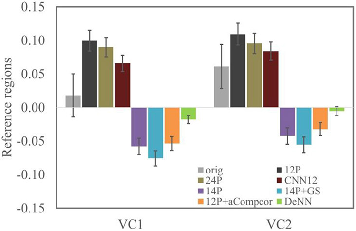
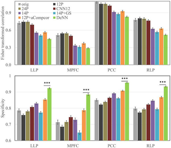
The connectivity (and standard error) between MPFC and two visual reference regions is shown in Fig. 6. 12P and 24P have significant positive bias for bilateral visual regions, and 14P, 14P+GS and 12P+aCompcor have significant negative bias for bilateral visual regions. Compared to original fMRI data, 12P and 24P regressors led to more severe positive bias, and 14P, 14P+GS and 12P+aCompcor led to negative bias in the reference regions. In contrast, DeNN achieved the most unbiased connectivity (close to zero) between MPFC and visual reference regions. The connectivity and its specificity values of the four positive ROIs are shown in Fig. 7. 12P and 24P had similar connectivity strength and specificity as original fMRI data. 14P, 14P+GS, 12P+aCompcor, and DeNN overall reduced connectivity strength and improved specificity compared to original fMRI data. DeNN had the highest specificity for all four positive ROIs with an average of 21.2% better than original fMRI data and an average of 8.2% above the second highest specificity achieved by 12P+aCompcor. A paired t-test between the specificity values achieved by DeNN and 12P+aCompcor showed that DeNN significantly improved specificity with p<10⁻¹⁰ for these four positive ROIs.

Fig. 6.

Mean connectivity between MPFC and bilateral visual regions using different denoising methods. The error bar indicates 2 × standard error.

Fig. 7.

Connectivity (top panel) and corresponding specificity (bottom panel) for four positive-correlated ROIs. The error bars are 2 × standard error. *** denotes p < 10⁻¹⁰.

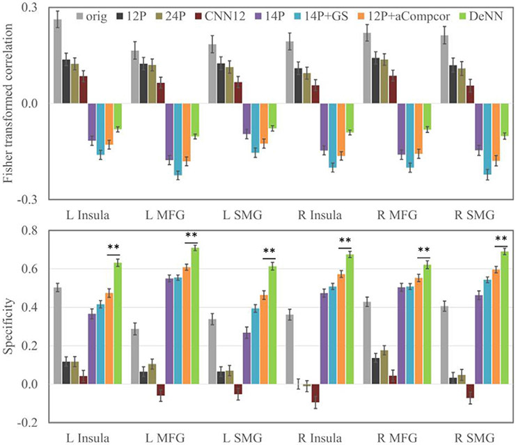
The connectivity and its specificity values of the six anticorrelated ROIs are shown in Fig. 8. Negative connectivity did not emerge in original data or the data only processed by realignment parameters and their variants. Global signal regression is well known to artificially introduce anticorrelation (Murphy et al., 2009), as expected, 14P+GS showed strongest anticorrelation among all methods. Consistent with the finding in Chai et al. (2012) that aCompcor is less likely to artificially introduce anticorrelation, 12P+aCompcor had weaker connectivity compared to 14P+GS, and DeNN had the weakest negative connectivity. In terms of specificity, DeNN had the highest specificity for all six anticorrelated ROIs with an average of 19.6% above the second highest specificity achieved by 12P+aCompcor. A paired t-test between the specificity values achieved by DeNN and 12P+aCompcor showed that DeNN has significantly improved specificity, with p<10⁻⁵ for these six negative ROIs. Compared to original fMRI data, 12P and 24P had decreased connectivity magnitude for negative ROIs and increased connectivity magnitude for the reference regions. Therefore, the specificity of these six negative ROIs for these two methods was considerably lower than the value of original fMRI data. Negative specificity was observed in 24P and CNN12, which was because the connectivity magnitude was lower than the connectivity magnitude of the reference regions.

Fig. 8.

The connectivity (top panel) and the corresponding specificity (bottom panel) for six negative ROIs. The error bars are 2 × standard error. ** denotes p < 10⁻⁵

Inter-subject homogeneity of whole-brain functional connectivity.

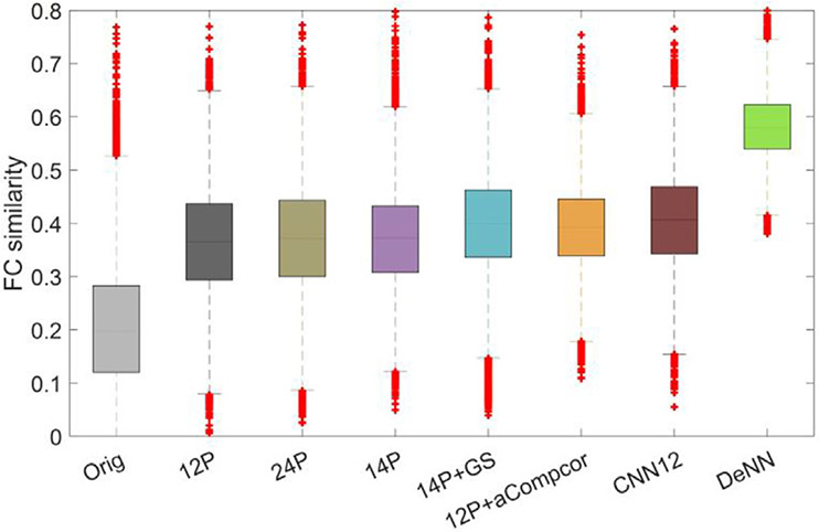
In addition to seed-based connectivity, we have calculated the whole-brain functional connectivity (FC) map using the AAL atlas (Tzourio-Mazoyer et al., 2002). Because the noise fluctuations in fMRI data could vary between subjects and between brain regions, “artificial connectivity” induced by these noise could lead to heterogeneous FC maps, improved between-subject similarity of FC maps is expected if a denoising technique correctly reduces the noise without considerably corrupting the signal in the data. Pair-wise Pearson’s correlation was used to evaluate the similarity of FC maps between each two subjects. The boxplot of FC similarity for different processed data is shown in Fig. 9. Compared to other processed datasets, DeNN substantially improved the inter-subject FC similarity. The mean similarity values are 0.207, 0.364, 0.371, 0.369, 0.397, 0.392, 0.405 and 0.582 for original, 12P, 24P, 14P, 14P+GS, 12P+aCompcor, CNN12 and DeNN processed data, respectively. The mean similarity achieved by DeNN is 181% higher than the value of the original data and 44% higher than the second highest similarity value achieved by CNN12. The set of 12 deep learning derived regressors in CNN12 shows improved inter-subject similarity over its traditional counterpart 12P and is slightly better than 12P+aCompcor but is less substantial than DeNN. We have also tested the FC maps with a functional atlas (Power et al., 2011) and observed consistent performance (see Figure S2). Furthermore, we have applied DeNN with the same network architecture, except that the number of time points for the first layer is adjusted correspondingly, on fast-acquisition fMRI data from HCP cohort and have found that DeNN retains the highest between-subject similarity (see Figure S3). With known intrinsic “functional connectivity” map in the simulated fMRI data (see Appendix), DeNN is consistently observed to have the best performance in uncovering the true connectivity map.

Fig. 9.

Pairwise similarity of functional connectivity between subjects.

Functional connectivity vs. motion summary measure.

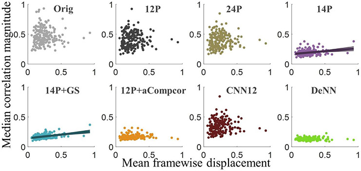
We have further tested the association between functional connectivity and motion summary measure. The scatter plots of median correlation magnitude (MCM) versus mean FD are shown in Fig. 10. Each dot represents the value from an individual subject. The MCM of each individual subject is defined as the median strength of the connectivities between 94 ROIs in the AAL atlas. MCM was observed to have a large variability between subjects in original, 12P, 24P, and CNN12 processed datasets. The variability was considerably reduced in 14P, 14P+GS, 12P+aCompcor, and DeNN. 14P and 14P+GS showed significant association between MCM and mean FD with p<0.001 and p<10⁻⁹, respectively, and all the other datasets did not have significant association between MCM and mean FD. Linear fitting was applied for 14P and 14P+GS data with a 95% confidence level, as shown in the figure.

Fig. 10.

Scatter plots of median correlation magnitude vs. mean framewise displacement. Each dot represents the value from an individual subject.

Group comparison based on network metrics.

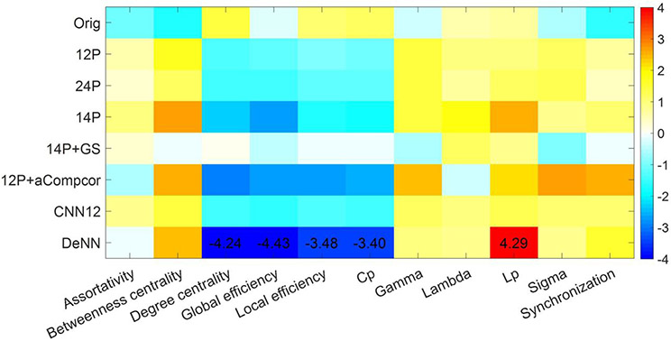
The question that naturally arises is whether the improved inter-subject homogeneity of FC maps would be detrimental for detecting the intrinsic difference between cognitively normal subjects and subjects with a neurodegenerative condition. Since the functional change in AD group is expected to be more severe and the functional change in eMCI is likely to be less detectable, we limit the group comparison to CN and AD groups in this study. Graph theoretical analysis as described in MATERIALS AND METHODS section was applied on the FC maps and the group difference between AD and CN was tested using 11 network metrics, with age, gender, handedness and education as covariates. The t statistical values of the group difference achieved by the seven processed datasets are shown in Fig. 11. Only the metrics passing p<0.05 after Bonferroni correction over the number of metrics and the number of datasets are marked with t value. Only with DeNN processed data, the AD group shows significant higher path length L_p and significant lower degree centrality, global efficiency, local efficiency, and clustering coefficient C_p. 14P and 12P+aCompcor show similar group difference, but the statistical significance does not pass the Bonferroni-corrected significance level p<0.05.

Fig. 11.

Group difference of graph theoretic metrics between cognitive normal subjects and subjects with AD. Only the metrics passing p values less than 0.05 after Bonferroni correction are marked with the t value.

4. Discussion

In this study, we have designed a subject-level deep neural network for denoising fMRI data as a data-driven non-regression technique. This network is optimized with fMRI time series as input, which does not require externally recorded data (e.g. physiological data) to model any specific noise sources. Therefore, DeNN can be widely applied for many existing fMRI datasets, particularly for those data that do not have externally recorded data available. In addition, once the network architecture is determined, DeNN automatically outputs denoised data without requiring human effort to identify noise fluctuation, which could be subjective and labor intensive. Since DeNN is trained for each subject separately with paired time series as input samples, this network is applicable for a study with a small sample size or even a single subject analysis.

By applying DeNN to resting-state fMRI data from the ADNI cohort, DeNN does not artificially induce connectivity (neither positive nor negative) between MPFC seed and visual cortex, and shows the highest specificity for positively correlated spontaneous fluctuations within the default mode network and for the anticorrelated fluctuations between regions in task positive network and PCC seed. The between-subject similarity of functional connectivity maps after DeNN denoising (mean similarity 0.582) is about three times of the similarity obtained by original time series (mean similarity 0.207) and about 1.5 times of the second highest similarity value (CNN12, mean similarity 0.405). Significant association between brain connectivity and motion summary measure is observed for 14P and 14P+GS but not for DeNN. Possibly because of the large between-subject variability, original, 12P, 24P and CNN12 data do not have significant association between brain connectivity and motion summary measure (see Fig. 10). We further demonstrate that the improved between-subject similarity in DeNN-processed data does not undermine, but strengthens, the group difference between cognitively normal subjects and subjects with AD in terms of graph-theoretical measures. The result from HCP data (see Supplementary) shows that DeNN is not limited to regular fMRI data but can also be applied on multi-band fast-acquisition (low TR) fMRI data. Overall, DeNN offers a new pathway towards improving the statistical power of fMRI and could strengthen the capability of fMRI in future neuroscience research and clinical practice.

DeNN vs. nuisance regression.

One main difference between DeNN and traditional nuisance regression methods is that DeNN takes advantage of the network structure to make it adaptive to the variability of noise fluctuation across the entire brain. While nuisance regression could adjust the weights of regressors for each brain region (or voxel), the regressors are fixed without considering potential spatial-dependent fluctuations caused by the same noise source. Our previous study (Yang et al., 2019) demonstrated that the same noise source could lead to a peak for some voxels but a dip for other voxels. In addition, adding more regressors to explain additional noise variance could potentially remove BOLD signal and induce unwanted noise variance (Chen et al., 2017). In contrast, DeNN is a non-regression-based denoising method. Naturally, DeNN does not involve the selection of regressors. Instead, after optimizing the model by disentangling GM time series from non-GM time series, DeNN automatically outputs the denoised time series with original time series as input.

Because 12P, 24P and CNN12 are observed as less effective methods in addressing the band-structure artifact, indicating similar noise fluctuation across the entire brain, this band structure could lead to “artificial positive connectivity” between brain regions. Therefore, 12P, 24P and CNN12, together with the original time series, have a stronger connectivity magnitude than other processed time series for the four positive ROIs in the default mode network. Such artificial connectivity could dominate over the intrinsic anticorrelation between PCC and the six negative-correlated ROIs in the task positive network, leading to erroneous positive connectivity. In contrast, DeNN and the denoising strategies with average time series or principal components extracted from fMRI data have correctly identified the anticorrelation. Consistent with the finding by Chai et al. (2012) that replacing the global signal with aCompcor components alleviates the overestimated anticorrelation, a similar finding is observed in our study. However, significant negative bias is still observed with aCompcor. Methods including 14P, 14P+GS, and 12P+aCompcor have significant negative bias in the reference regions, which is not the case for DeNN. This phenomenon could explain why DeNN has weaker anticorrelation compared to these three methods, and the anticorrelation obtained by DeNN more likely reflects the intrinsic connectivity strength of neural fluctuations because of DeNN’s unbiased connectivity estimation in the reference regions.

DeNN vs. previous deep neural network denoising.

DeNN is distinct from our two recently developed deep learning denoising methods, one for resting-state (Yang et al., 2019) and the other one for task fMRI data (Yang et al., 2020b). In contrast to those two methods, a novel time-dependent fully-connected layer is designed in DeNN to effectively remove noise in the data. Unlike Yang et al. (2019) applied deep learning to derive nuisance regressors, DeNN is not a regression method, and the network outputs the denoised fMRI data directly. The task design used in task fMRI denoising (Yang et al., 2020b) is not required in DeNN, thus DeNN perfectly fits for resting-state fMRI data.

The proposed time-dependent fully-connected layer plays a critical role in boosting the performance. The temporal convolutional layer and long short-term memory (LSTM) layer are the two kinds of layers used in our previous studies (Yang et al., 2019; Yang et al., 2020b), which take neighboring time points to inform the current time point. These two layers are invariant to the time point, thus they could be more effective for reducing periodic or pseudoperiodic noise induced by cardiac or respiratory oscillations. The gray plot of original time series shows that the noise variance at each time point can be unique, a network without the temporally dependent layer is likely to be less efficient in addressing these irregular noise (see gray plots in the Supplementary). DeNN takes advantage of the time-dependent fully-connected layer to make it temporally adaptive. Because the network for task fMRI data discards any fluctuation irrelevant to the task (Yang et al., 2020b), this problem is likely more severe in the network for resting-state fMRI data (Yang et al., 2019). To overcome this obstacle, the time-dependent fully-connected layer is proposed in DeNN to reduce distinct noise fluctuation for each time point separately. In addition, DeNN outputs the denoised time series directly instead of optimizing a set of spatially independent nuisance regressors, thereby increasing DeNN’s flexibility and capability to differentiate spatial-varying noise from the BOLD signal. Certainly, LSTM potentially can be an additional part of DeNN or the replacement of temporal convolutional layer used in current DeNN architecture, however, an LSTM layer is not expected to make substantial performance difference because of its similar temporal property as a temporal convolutional layer.

Limitation and future study.

The parameter size for the time-dependent fully connected layer linearly increases with the number of time points, leading to more expensive computational time for longer time series. Noise reduction for 135 time points (ADNI data) requires approximately fifteen minutes for one subject, and noise reduction for 1200 time points (HCP data) requires approximately six hours for one subject on a workstation with a single Tesla K40c GPU card. A large sample study may require parallel computation, particularly for data with the number of time points larger than 1000. In addition, optimal noise reduction for a set of new data could require adjusting the depth of the network or the width of each layer. However, the current network architecture performs adequately for two distinct datasets, suggesting that the network is insensitive to different acquisition parameters. In addition, DeNN currently is only validated with connectivity analysis, the application of DeNN for other types of analysis, e.g. fALFF (Zou et al., 2008), requires further investigation. Researchers should first validate the applicability of DeNN when using it for non-connectivity analysis.

While DeNN was designed for resting-state fMRI, it can be applied to denoise task fMRI data as well. The deep neural network targeted at denoising task fMRI data (Yang et al., 2020b) is likely to provide more robust activation maps than DeNN because a task design matrix is used in Yang et al. (2020b), with the drawback that the data is required to be denoised again for a different task design of interest. Instead, DeNN is applied based on fMRI data itself without specifying a task design. Furthermore, DeNN is likely to be a better choice for denoising passive-viewing task fMRI data, where specifying a task design is less feasible, if not impossible. Currently DeNN is only evaluated with resting-state fMRI data, and its performance on task fMRI data remains to be investigated.

5. Summary

Our current results demonstrate the feasibility of using artificial intelligence to denoise fMRI data by disentangling the time series between gray matter tissue and non-gray matter tissue. This automated fMRI denoising neural network is generally applicable without requiring externally recorded data. The proposed time-distributed fully connected layer makes the network spatially and temporally adaptive to the noise in the data. The network is applied at the subject-level, therefore, it is completely feasible for a study with a small sample size. It is insensitive to fMRI acquisition parameters and can be applied both on standard and fast-acquisition fMRI data. We have shown that the denoising network reveals no connectivity between functionally uncorrelated regions and has the highest specificity for the positive correlation within the default model network and the anticorrelation between networks. Furthermore, this network substantially increases the homogeneity of functional connectivity maps and strengthens the statistical power of fMRI data in detecting the group difference between cognitively normal subjects and subjects with AD.

Appendix

Simulation

Instead of generating noise from scratch, we use non-GM time series extracted from real fMRI data to define noise data without any BOLD signal. To simulate the neural signal in GM, we use boxcar functions (specified below) that are convolved with the canonical hemodynamic response function. With this definition, the simulated time series y with 135 time points can be written as

$$\mathit{y}=(1-f)\ast {\mathit{y}}_{\text{signal}}+f\ast {\mathit{y}}_{\text{noise}},$$ (A1)

where f is the noise fraction. Specifically, the noise y_noise is generated by randomly selecting one time series y_non–GM from non-GM voxels of real resting-state data from one subject, and adding additional white Gaussian noise according to the equation

$${\mathit{y}}_{\text{noise}}={\mathit{y}}_{\text{non}-\text{GM}}+0.05\ast \mathbf{N}(0,\mathit{I}),$$ (A2)

where N(0, I) represents a normal random vector following a Gaussian distribution with mean 0 and identity covariance matrix I. The BOLD signal in a voxel is defined to be

$${\mathit{y}}_{\text{signal}}=\mathit{S}\cdot ({\mathit{w}}_i+0.1\ast \mathbf{N}(0,\mathit{I})),i=\text{randi}(8).$$ (A3)

Fig. A1.

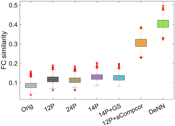
Boxplot of FC similarity between true FC map and FC map estimated with denoised time series.

The index i is a positive random integer with maximum value 8 and S = [s₁, …, s₈] contains 8 simulated BOLD components where each vector s_i is generated by convolving a random binary vector (consisting of 105 zeros and 30 ones) with the canonical hemodynamic response function.The weight vectors w_i, i = 1, … , 8 are given by

$$\mathbf{W}=[{\mathit{w}}_1,{\mathit{w}}_2,\dots ,{\mathit{w}}_7,{\mathit{w}}_8]=\left[\begin{array}{cccccccc}0.5\hfill & 0\hfill & 0\hfill & 0\hfill & 0.5\hfill & 0\hfill & \hfill 0\hfill & \hfill 0\hfill \\ 0.5\hfill & 0\hfill & 0\hfill & 0\hfill & 0\hfill & 0.5\hfill & \hfill 0\hfill & \hfill 0\hfill \\ 0\hfill & 0.5\hfill & 0\hfill & 0\hfill & 0.5\hfill & 0\hfill & \hfill 0\hfill & \hfill 0\hfill \\ 0\hfill & 0.5\hfill & 0\hfill & 0\hfill & 0\hfill & 0.5\hfill & \hfill 0\hfill & \hfill 0\hfill \\ 0\hfill & 0\hfill & 0.5\hfill & 0\hfill & 0\hfill & 0\hfill & \hfill 0.5\hfill & \hfill 0\hfill \\ 0\hfill & 0\hfill & 0.5\hfill & 0\hfill & 0\hfill & 0\hfill & \hfill 0\hfill & \hfill 0.5\hfill \\ 0\hfill & 0\hfill & 0\hfill & 0.5\hfill & 0\hfill & 0\hfill & \hfill 0.5\hfill & \hfill 0\hfill \\ 0\hfill & 0\hfill & 0\hfill & 0.5\hfill & 0\hfill & 0\hfill & \hfill 0\hfill & \hfill 0.5\hfill \end{array}\right].$$ (A4)

80% of GM voxels are simulated to have BOLD signal (named informative voxels) and the remaining 20% of GM voxels do not carry any BOLD signal. The scripts for simulation are publicly available at https://github.com/pipiyang/DeNN.

We have run DeNN on simulated data with the same architecture for ADNI data. To evaluate how well each denoising strategy can uncover the intrinsic connectivity between informative voxels, we randomly select 100 informative voxels and calculate the “functional connectivity” (FC) map between these 100 voxels with the true signal y_signal, original simulated time series y, and different denoised time series. Then we have calculated the similarity between FC map from true signal and FC map from original or denoised time series after vectorising the FC map, namely corr(FC_signal, FC_timeseries). The noise fraction is specified as 0.8 to have the similarity of simulated original data close to the inter-subject similarity of real original fMRI data. We have repeated selecting 100 informative voxels randomly for 1000 times and the boxplot of the similarity is shown in Fig. A1. Substantial improvement is observed with DeNN processed data, which is consistent with real data.

References

- Anderson JS, Druzgal TJ, Lopez-Larson M, Jeong EK, Desai K, Yurgelun-Todd D, 2011. Network anticorrelations, global regression, and phase - shifted soft tissue correction. Hum. Brain Mapp 32, 919–934. [DOI] [PMC free article] [PubMed] [Google Scholar]
- Behzadi Y, Restom K, Liau J, Liu TT, 2007. A component based noise correction method (CompCor) for BOLD and perfusion based fMRI. Neuroimage 37, 90–101. [DOI] [PMC free article] [PubMed] [Google Scholar]
- Bianciardi M, Fukunaga M, van Gelderen P, Horovitz SG, de Zwart JA, Shmueli K, Duyn JH, 2009. Sources of functional magnetic resonance imaging signal fluctuations in the human brain at rest: a 7 T study. Magn. Reson. Imaging 27, 1019–1029. [DOI] [PMC free article] [PubMed] [Google Scholar]
- Birn RM, Diamond JB, Smith MA, Bandettini PA, 2006. Separating respiratory-variation-related fluctuations from neuronal-activity-related fluctuations in fMRI. Neuroimage 31, 1536–1548. [DOI] [PubMed] [Google Scholar]
- Birn RM, Smith MA, Jones TB, Bandettini PA, 2008. The respiration response function: the temporal dynamics of fMRI signal fluctuations related to changes in respiration. Neuroimage 40, 644–654. [DOI] [PMC free article] [PubMed] [Google Scholar]
- Biswal B, Zerrin Yetkin F, Haughton VM, Hyde JS, 1995. Functional connectivity in the motor cortex of resting human brain using echo-planar MRI. Magn. Reson. Med 34, 537–541. [DOI] [PubMed] [Google Scholar]
- Boubela RN, Kalcher K, Huf W, Kronnerwetter C, Filzmoser P, Moser E, 2013. Beyond noise: using temporal ICA to extract meaningful information from high-frequency fMRI signal fluctuations during rest. Front. Hum. Neurosci 7, 168. [DOI] [PMC free article] [PubMed] [Google Scholar]
- Caballero-Gaudes C, Reynolds RC, 2017. Methods for cleaning the BOLD fMRI signal. Neuroimage 154, 128–149. [DOI] [PMC free article] [PubMed] [Google Scholar]
- Chai XJ, Castañón AN, Öngür D, Whitfield-Gabrieli S, 2012. Anticorrelations in resting state networks without global signal regression. Neuroimage 59, 1420–1428. [DOI] [PMC free article] [PubMed] [Google Scholar]
- Chang C, Cunningham JP, Glover GH, 2009. Influence of heart rate on the BOLD signal: the cardiac response function. Neuroimage 44, 857–869. [DOI] [PMC free article] [PubMed] [Google Scholar]
- Chen JE, Glover GH, 2015. BOLD fractional contribution to resting-state functional connectivity above 0.1 Hz. Neuroimage 107, 207–218. [DOI] [PMC free article] [PubMed] [Google Scholar]
- Chen JE, Jahanian H, Glover GH, 2017. Nuisance regression of high-frequency functional magnetic resonance imaging data: denoising can be noisy. Brain Connect. 7, 13–24. [DOI] [PMC free article] [PubMed] [Google Scholar]
- Cordes D, Haughton VM, Arfanakis K, Carew JD, Turski PA, Moritz CH, Quigley MA, Meyerand ME, 2001. Frequencies contributing to functional connectivity in the cerebral cortex in “resting-state” data. Am. J. Neuroradiol 22, 1326–1333. [PMC free article] [PubMed] [Google Scholar]
- Fox MD, Snyder AZ, Vincent JL, Corbetta M, Van Essen DC, Raichle ME, 2005. The human brain is intrinsically organized into dynamic, anticorrelated functional networks. Proc. Natl. Acad. Sci 102, 9673–9678. [DOI] [PMC free article] [PubMed] [Google Scholar]
- Friston KJ, Williams S, Howard R, Frackowiak RS, Turner R, 1996. Movement-related effects in fMRI time-series. Magn. Reson. Med 35, 346–355. [DOI] [PubMed] [Google Scholar]
- Glorot X, Bengio Y, 2010. Understanding the difficulty of training deep feedforward neural networks. In: Proceedings of the Thirteenth International Conference On Artificial Intelligence And Statistics, pp. 249–256. [Google Scholar]
- Glover GH, Li TQ, Ress D, 2000. Image-based method for retrospective correction of physiological motion effects in fMRI: RETROICOR. Magn. Reson. Med 44, 162–167 An Official Journal of the International Society for Magnetic Resonance in Medicine. [DOI] [PubMed] [Google Scholar]
- Griffanti L, Salimi-Khorshidi G, Beckmann CF, Auerbach EJ, Douaud G, Sexton CE, Zsoldos E, Ebmeier KP, Filippini N, Mackay CE, 2014. ICA-based artefact removal and accelerated fMRI acquisition for improved resting state network imaging. Neuroimage 95, 232–247. [DOI] [PMC free article] [PubMed] [Google Scholar]
- Harvey AK, Pattinson KT, Brooks JC, Mayhew SD, Jenkinson M, Wise RG, 2008. Brainstem functional magnetic resonance imaging: disentangling signal from physiological noise. J. Magn. Reson. Imaging 28, 1337–1344 An Official Journal of the International Society for Magnetic Resonance in Medicine. [DOI] [PubMed] [Google Scholar]
- Jo HJ, Saad ZS, Simmons WK, Milbury LA, Cox RW, 2010. Mapping sources of correlation in resting state FMRI, with artifact detection and removal. NeuroImage 52, 571–582. [DOI] [PMC free article] [PubMed] [Google Scholar]
- Johnstone T, Ores Walsh KS, Greischar LL, Alexander AL, Fox AS, Davidson RJ, Oakes TR, 2006. Motion correction and the use of motion covariates in multiple - subject fMRI analysis. Hum. Brain Mapp 27, 779–788. [DOI] [PMC free article] [PubMed] [Google Scholar]
- Kay K, Rokem A, Winawer J, Dougherty R, Wandell B, 2013. GLMdenoise: a fast, automated technique for denoising task-based fMRI data. Front. Neurosci 7, 247. [DOI] [PMC free article] [PubMed] [Google Scholar]
- Kingma DP, Ba J, 2014. Adam: A method for stochastic optimization. arXiv preprint arXiv:1412.6980. [Google Scholar]
- Marblestone AH, Wayne G, Kording KP, 2016. Toward an integration of deep learning and neuroscience. Front. Comput. Neurosci 10, 94. [DOI] [PMC free article] [PubMed] [Google Scholar]
- Murphy K, Birn RM, Bandettini PA, 2013. Resting-state fMRI confounds and cleanup. Neuroimage 80, 349–359. [DOI] [PMC free article] [PubMed] [Google Scholar]
- Murphy K, Birn RM, Handwerker DA, Jones TB, Bandettini PA, 2009. The impact of global signal regression on resting state correlations: are anti-correlated networks introduced? Neuroimage 44, 893–905. [DOI] [PMC free article] [PubMed] [Google Scholar]
- Power JD, Barnes KA, Snyder AZ, Schlaggar BL, Petersen SE, 2012. Spurious but systematic correlations in functional connectivity MRI networks arise from subject motion. Neuroimage 59, 2142–2154. [DOI] [PMC free article] [PubMed] [Google Scholar]
- Power JD, Cohen AL, Nelson SM, Wig GS, Barnes KA, Church JA, Vogel AC, Laumann TO, Miezin FM, Schlaggar BL, 2011. Functional network organization of the human brain. Neuron 72, 665–678. [DOI] [PMC free article] [PubMed] [Google Scholar]
- Power JD, Plitt M, Gotts SJ, Kundu P, Voon V, Bandettini PA, Martin A, 2018. Ridding fMRI data of motion-related influences: Removal of signals with distinct spatial and physical bases in multiecho data. Proc. Natl. Acad. Sci 115, E2105–E2114. [DOI] [PMC free article] [PubMed] [Google Scholar]
- Pruim RH, Mennes M, van Rooij D, Llera A, Buitelaar JK, Beckmann CF, 2015. ICA-AROMA: A robust ICA-based strategy for removing motion artifacts from fMRI data. Neuroimage 112, 267–277. [DOI] [PubMed] [Google Scholar]
- Saad ZS, Gotts SJ, Murphy K, Chen G, Jo HJ, Martin A, Cox RW, 2012. Trouble at rest: how correlation patterns and group differences become distorted after global signal regression. Brain Connect. 2, 25–32. [DOI] [PMC free article] [PubMed] [Google Scholar]
- Salimi-Khorshidi G, Douaud G, Beckmann CF, Glasser MF, Griffanti L, Smith SM, 2014. Automatic denoising of functional MRI data: combining independent component analysis and hierarchical fusion of classifiers. Neuroimage 90, 449–468. [DOI] [PMC free article] [PubMed] [Google Scholar]
- Satterthwaite TD, Elliott MA, Gerraty RT, Ruparel K, Loughead J, Calkins ME, Eickhoff SB, Hakonarson H, Gur RC, Gur RE, 2013. An improved framework for confound regression and filtering for control of motion artifact in the preprocessing of resting-state functional connectivity data. Neuroimage 64, 240–256. [DOI] [PMC free article] [PubMed] [Google Scholar]
- Shmueli K, van Gelderen P, de Zwart JA, Horovitz SG, Fukunaga M, Jansma JM, Duyn JH, 2007. Low-frequency fluctuations in the cardiac rate as a source of variance in the resting-state fMRI BOLD signal. Neuroimage 38, 306–320. [DOI] [PMC free article] [PubMed] [Google Scholar]
- Tijssen RH, Jenkinson M, Brooks JC, Jezzard P, Miller KL, 2014. Optimizing RetroICor and RetroKCor corrections for multi-shot 3D FMRI acquisitions. NeuroImage 84, 394–405. [DOI] [PMC free article] [PubMed] [Google Scholar]
- Tzourio-Mazoyer N, Landeau B, Papathanassiou D, Crivello F, Etard O, Delcroix N, Mazoyer B, Joliot M, 2002. Automated anatomical labeling of activations in SPM using a macroscopic anatomical parcellation of the MNI MRI single-subject brain. Neuroimage 15, 273–289. [DOI] [PubMed] [Google Scholar]
- Van Dijk KR, Hedden T, Venkataraman A, Evans KC, Lazar SW, Buckner RL, 2010. Intrinsic functional connectivity as a tool for human connectomics: theory, properties, and optimization. J. Neurophysiol 103, 297–321. [DOI] [PMC free article] [PubMed] [Google Scholar]
- Van Dijk KR, Sabuncu MR, Buckner RL, 2012. The influence of head motion on intrinsic functional connectivity MRI. Neuroimage 59, 431–438. [DOI] [PMC free article] [PubMed] [Google Scholar]
- Van Essen DC, Smith SM, Barch DM, Behrens TE, Yacoub E, Ugurbil K, Consortium, W.-M.H., 2013. The WU-Minn human connectome project: an overview. Neuroimage 80, 62–79. [DOI] [PMC free article] [PubMed] [Google Scholar]
- Wang J, Wang X, Xia M, Liao X, Evans A, He Y, 2015. GRETNA: a graph theoretical network analysis toolbox for imaging connectomics. Front. Hum. Neurosci 9, 386. [DOI] [PMC free article] [PubMed] [Google Scholar]
- Weissenbacher A, Kasess C, Gerstl F, Lanzenberger R, Moser E, Windischberger C, 2009. Correlations and anticorrelations in resting-state functional connectivity MRI: a quantitative comparison of preprocessing strategies. Neuroimage 47, 1408–1416. [DOI] [PubMed] [Google Scholar]
- Yang Z, Zhuang X, Mishra V, Sreenivasan K, Cordes D, 2020a. CAST: A multi-scale convolutional neural network based automated hippocampal subfield segmentation toolbox. Neuroimage, 116947. [DOI] [PMC free article] [PubMed] [Google Scholar]
- Yang Z, Zhuang X, Screenivasan KR, Mishra VR, Cordes D, 2019. Robust motion regression of resting-state data using a convolutional neural network model. Front. Neurosci 13, 169. [DOI] [PMC free article] [PubMed] [Google Scholar]
- Yang Z, Zhuang X, Sreenivasan K, Mishra V, Curran T, Cordes D, 2020b. A robust deep neural network for denoising task-based fMRI data: An application to working memory and episodic memory. Med. Image Anal 60, 101622. [DOI] [PMC free article] [PubMed] [Google Scholar]
- Zou Q-H, Zhu C-Z, Yang Y, Zuo X-N, Long X-Y, Cao Q-J, Wang Y-F, Zang Y-F, 2008. An improved approach to detection of amplitude of low-frequency fluctuation (ALFF) for resting-state fMRI: Fractional ALFF. J. Neurosci. Methods 172, 137–141. [DOI] [PMC free article] [PubMed] [Google Scholar]
Associated Data
This section collects any data citations, data availability statements, or supplementary materials included in this article.